Infrared Small Marine Target Detection Based on Spatiotemporal Dynamics Analysis

Abstract

It is a big challenge to detect and track small infrared marine targets in non-stationary and time-varying sea clutter because the signal is too strong to be estimated. Based on the phenomenon that sea clutter spreads not only in the temporal domain but also in the spatial domain, this paper proposes an infrared small marine target detection algorithm based on spatiotemporal dynamics analysis to improve the performances of sea clutter suppression and target detection. The moving sea clutter is modeled as the spatial-temporal phase space, and the dynamical parameters of the sea clutter in the spatiotemporal domain are extracted from the sea clutter image sequence. Afterwards, the temporal dynamics reconstruction function and the spatial dynamics reconstruction function are built based on these extracted dynamical parameters. Furthermore, the space-time coupling coefficient and the spatiotemporal dynamics reconstruction function are estimated by means of a radial basis function (RBF) neural network to reconstruct the propagation regularity of the moving sea clutter. Finally, the sea clutter is suppressed by subtracting the estimated image from the original image, and then the target is detected in the suppressed image using the constant false alarm rate (CFAR) criteria. Some experiments on the small marine target in various fluctuating sea clutter image sequences are induced, and the experimental results show that the proposed algorithm could achieve outstanding performances in sea clutter suppression and small target detection.

1. Introduction

Marine target detection and tracking in sea clutter is an important task for airborne and shipborne tracking systems, which are usually equipped with infrared, radar, and SAR [1,2,3]. The infrared tracking system has the advantages of good concealment, strong anti-electromagnetic interference ability, and high angular resolution. However, the infrared target for sea clutter continuously changes, including signal-to-noise, contrast, and even shape [4], and usually undulates dynamically. In contrast to the static background of the ground and sky, there are surges similar to a sine wave or storm without regular structure in the undulating sea clutter that are strong, non-stationary, and even time-varying [5]. Moreover, the power of sea clutter may be equal to or even greater than that of a small target in an infrared sea clutter image in the case of strong scale light [6]. The undulating sea clutter is still a major problem for infrared small target detection and tracking, and how to effectively detect the infrared marine target in sea clutter is a big challenge for the existing small target detection algorithms [7,8,9].

In traditional methods, the sea clutter is regarded as a completely random signal, and then the probability distribution of the sea clutter is established for target detection and recognition. It is well known that the trailing of the fluctuating sea clutter is a unique phenomenon that has been widely applied in target recognition. So far, the Log-Normal distribution [10], the Weibull distribution [10], and the K distribution [11] have been developed to describe the trailing phenomenon, and these probability distributions can approximate the sea clutter to a certain extent. However, these statistical algorithms simulated by the probability distribution have failed to describe the shape of sea clutter, and they are not effective enough to detect the small infrared marine targets submerged in sea clutter.

In addition, some target detection methods regard sea clutter as non-stationary random signals, and spatial filters, such as wavelet analysis [12] and gray-scale morphology [13], are used to estimate the sea clutter signal. Compared to small infrared targets, sea clutter is usually a low-frequency signal because it has a strong correlation in the space domain and time domain, and it could be suppressed to the greatest extent as Gaussian white noise. In Gaussian white noise, small targets can be distinct enough to be detected because of their strong signal amplitude. Nevertheless, the undulating sea clutter has such an incredibly wide frequency range that it covers more than the frequency of the target, and it is difficult for these filters to fit the irregular structure of sea clutter. Furthermore, the temporal filter, such as the third-order recursive filter [14], is so sensitive to the motion parameters that it is hard to achieve completely satisfactory performance because the fluctuant sea clutter propagates at various speeds. As a viscous fluid, sea clutter propagates continuously in the spatiotemporal domain, and its corresponding infrared image sequence is also a non-stationary signal in the spatiotemporal domain. Therefore, the classical methods could not efficiently describe the physical characteristics of a sea clutter image sequence.

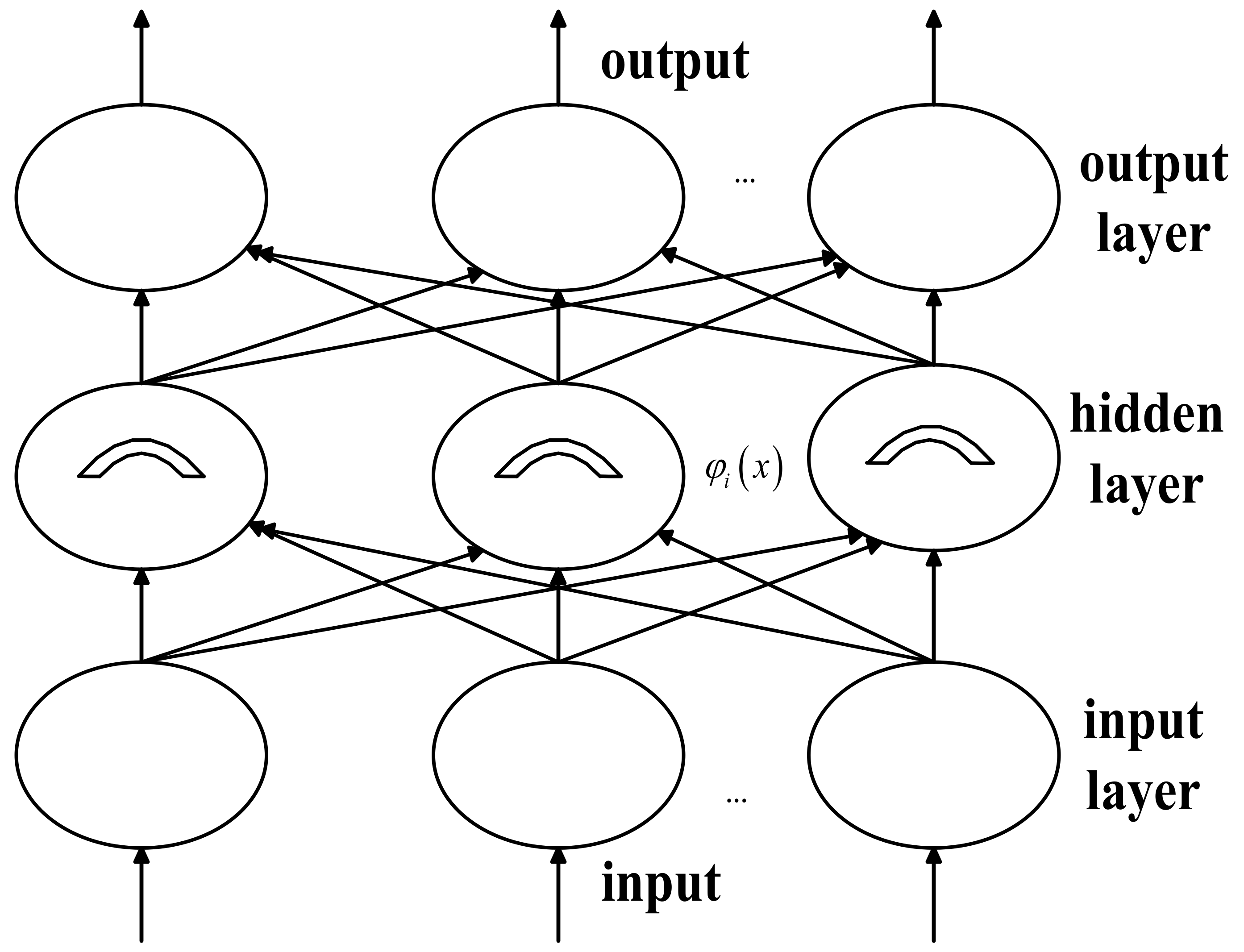
To improve the performance of small target detection, the characteristics of the undulating sea clutter have been studied. In the field of radar detection, sea clutter has been modeled as a nonlinear system [15,16,17] and is estimated by means of a radial basis function (RBF) artificial neural network [18]. It is well known that the amplitude of the infrared image is the product of incident light and reflected light. The incident light depends on the light source and is generally uniform, while the reflected light is usually determined by the spatial structure and material properties of the reflector itself. For the infrared sea clutter image, the details are primarily determined by the reflected light, namely, the spatiotemporal structure and the temperature difference at various depths, and the former corresponds to the undulating sea clutter [19,20]. Driven by a variety of forces, such as wind, gravity, and friction, the sea wave spreads continuously in the spatiotemporal domain. A seawater particle vibrates periodically or quasi-periodically near its equilibrium position under the action of gravity. Meanwhile, due to the continuity of the seawater fluid, the particles near the vibrating particle would also fluctuate, and the vibration would spread further. Therefore, the fluctuation of the sea wave propagates in a certain direction, and the corresponding infrared image also fluctuates dynamically [21,22]. In fact, driven by the approximation rule, the seawater vibrates under a certain degree of dynamics, and the infrared sea clutter image has corresponding dynamical characteristics in the spatiotemporal domain. The temporal dynamical characteristics of the infrared sea clutter image were verified by testing the maximum Lyapunov exponent and the correlation dimension [23]. Nevertheless, the spatial structure and material properties of the target, such as a ship, usually do not change, which results in almost constant reflected light, so the dynamical characteristics of sea clutter will stop at the place where the target appears. The remarkable difference between the fluctuating seawater and the stationary target was applied, and the target detection performance significantly improved [24,25]. Nevertheless, the existing achievements in sea clutter estimation usually focus on its temporal dynamics, while the research on its spatial dynamics is insufficient.

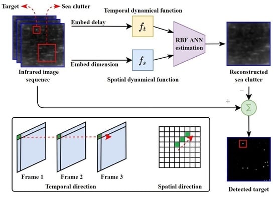
As mentioned above, sea waves move continuously and regularly in the space domain; the spatial dynamics are always accompanied by the temporal dynamics because the sea wave moves continuously and propagates regularly in the space domain. Therefore, the dynamical characteristics in the spatial-temporal domain could simultaneously enhance the sea clutter suppression and improve the target detection performance. This paper proposes an algorithm for detecting small infrared marine targets in sea clutter based on spatiotemporal dynamics analysis.

The remainder of the paper is organized as follows: Section 2 discusses how to extract the dynamical parameters of infrared sea clutter image sequences, and Section 3 jointly reconstructs the dynamical phase space of sea clutter in the spatiotemporal domain. In Section 4, the infrared sea clutter image is estimated using spatiotemporal dynamical parameters. Some experiments are included in Section 5 to evaluate its target detection performance in sea clutter, and the conclusions are given in Section 6.

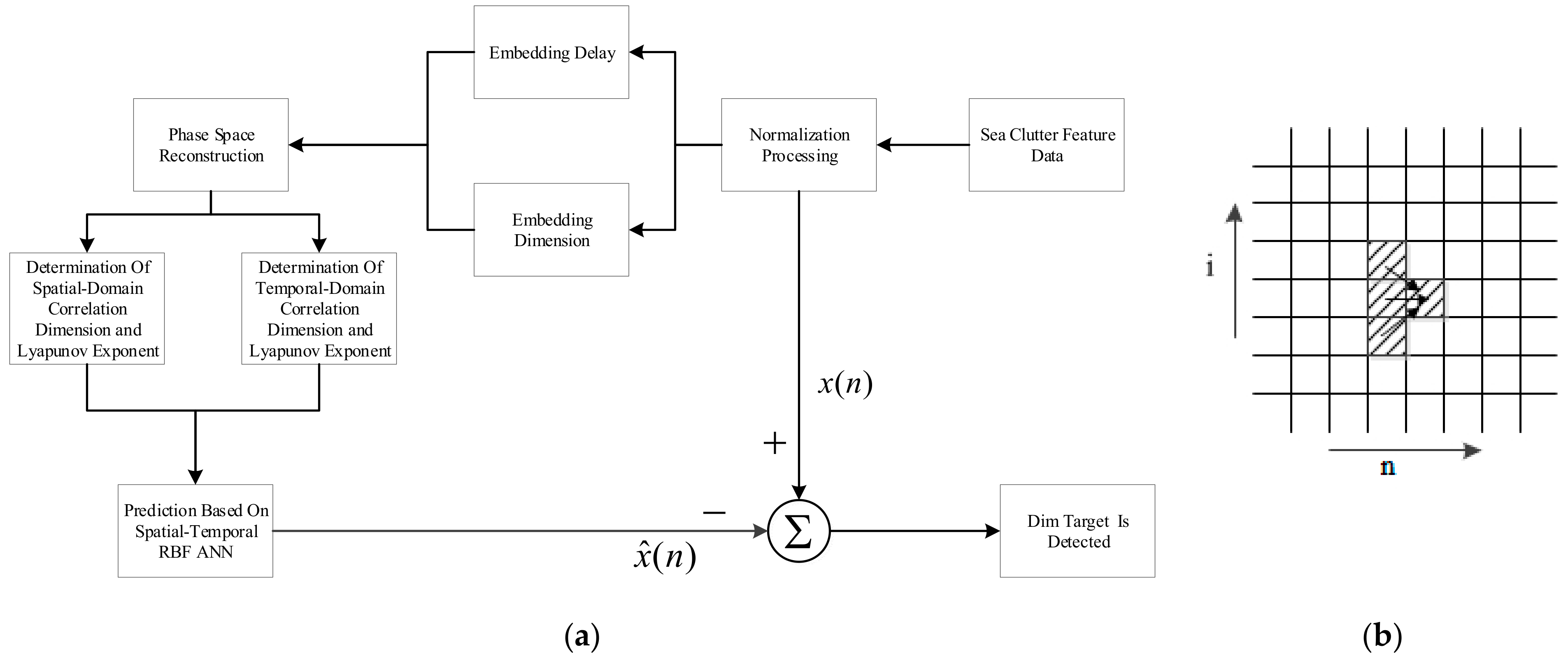
2. Spatiotemporal Dynamical Parameter Extraction

The sea clutter propagates in a certain direction in the spatiotemporal domain because of the asymmetry of pressures on both sides of the wave crest, since the windward side is blown by the wind. The uneven pressure is absorbed by the seawater, and then the absorbed energy is consumed through its propagation. Therefore, the balance between force absorption and energy consumption determines the growth and attenuation of sea waves, and the sea clutter propagates dynamically in a certain direction in the spatiotemporal domain.

The undulating sea clutter’s dynamical phenomenon is jointly and interactively caused by various forces. By extending the temporal-spatial space, its phase space could be fully reconstructed to reveal the information. If the delay time and embedded dimension are properly selected, its topology is equivalent to the original system [26,27].

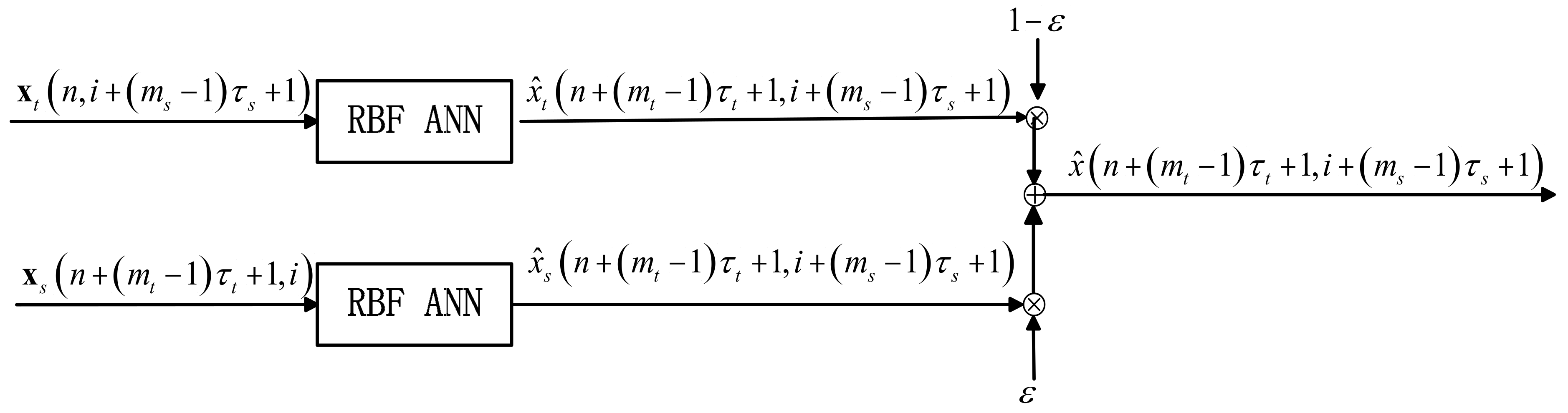
As is known to all, sea clutter propagates in a certain direction in the temporal-spatial domain. Therefore, the dynamical parameters in the temporal domain and the spatial domain should be extracted from the temporal sequence data and the spatial sequence data, respectively. After determining the dynamics of sea clutter, the temporal phase space and the spatial phase space could be reconstructed based on these dynamical parameters. Afterwards, the radial basis function neural network is used to estimate the space-time coupling coefficient, and then the spatial dynamical function and the temporal dynamical function jointly reconstruct the propagation regularity of the moving sea clutter.

2.1. Time Serial Data Extraction

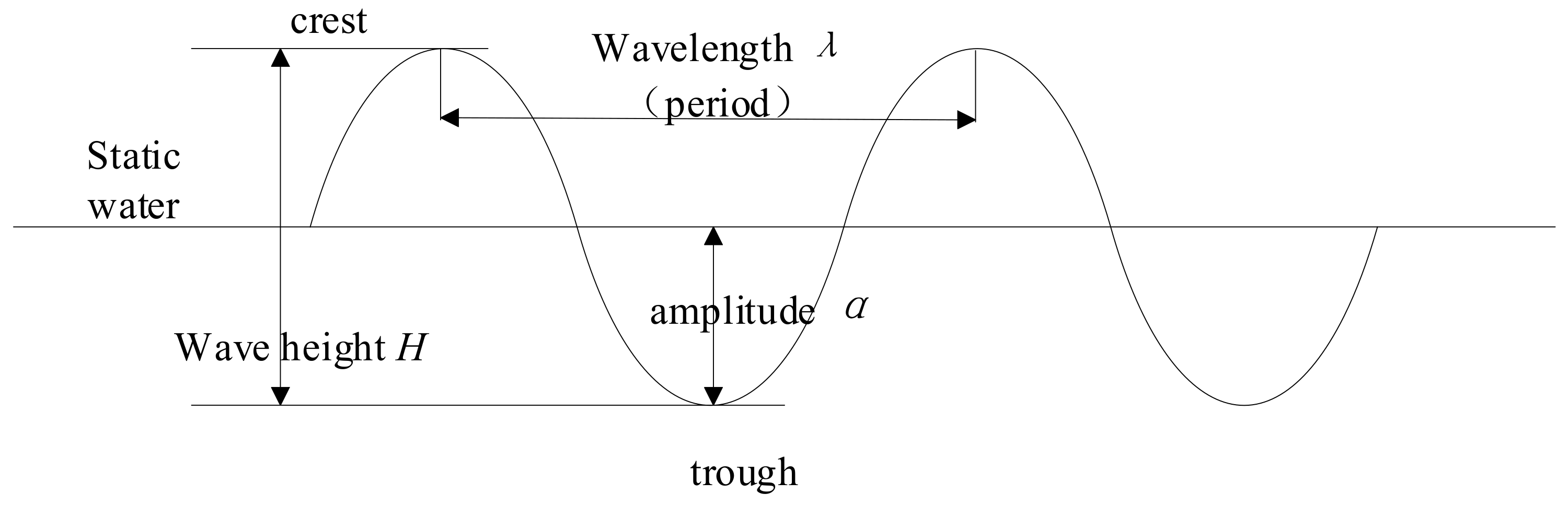
The particles of seawater vibrate periodically or quasi-periodically due to gravity near their equilibrium position or the static water. In Figure 1, the highest point and the lowest point are the crest and the trough, respectively, and the period between two consecutive crests is the wavelength $\lambda$. In addition to gravity, the particles of seawater are also driven by a variety of forces, such as wind, and their vibration is not completely periodic but has a certain dynamical characteristic.

For the infrared sea clutter image, its details are mainly determined by the spatial structure and the temperature difference, and it also has the same dynamical characteristics as seawater. For each pixel of the infrared sea clutter image, the change in its intensity with time could reflect the fluctuation of the seawater. The time series data selected at the same location as the continuous image can represent the fluctuation of the seawater accordingly. For example, when the camera is fixed, the time serial data $x_t\left(n,i\right)$ of the infrared sea clutter image could be selected at the same pixel.

When the sea clutter is dynamic, the appropriate delay time and embedded dimension of the time serial data $x_t\left(n,i\right)$, that is, the time trajectory, can be used to reconstruct its phase space, and the phase point [28] in the reconstructed trajectory is denoted as

$$Y_t(n,i) =\left\{x(n,i),x(n+{\tau }_t,i),\cdots ,x\left(n+ (m_t-1){\tau }_t,i \right)\right\}$$

(1)

where $n$ is the number of the image frame, $i$ is the pixel of the sea clutter image, and ${\tau }_t$ and $m_t$ are the delay time and the embedded dimension, respectively.

2.2. Space Serial Data Extraction

The particles near the vibrating particle would also fluctuate due to the continuity of the seawater fluid, and the vibration would spread farther. Therefore, the sea wave propagation along a certain direction leads to the dynamical change of the infrared image of sea clutter in space, so the spatial serial data should be selected in the direction of the fluctuating sea clutter movement accordingly.

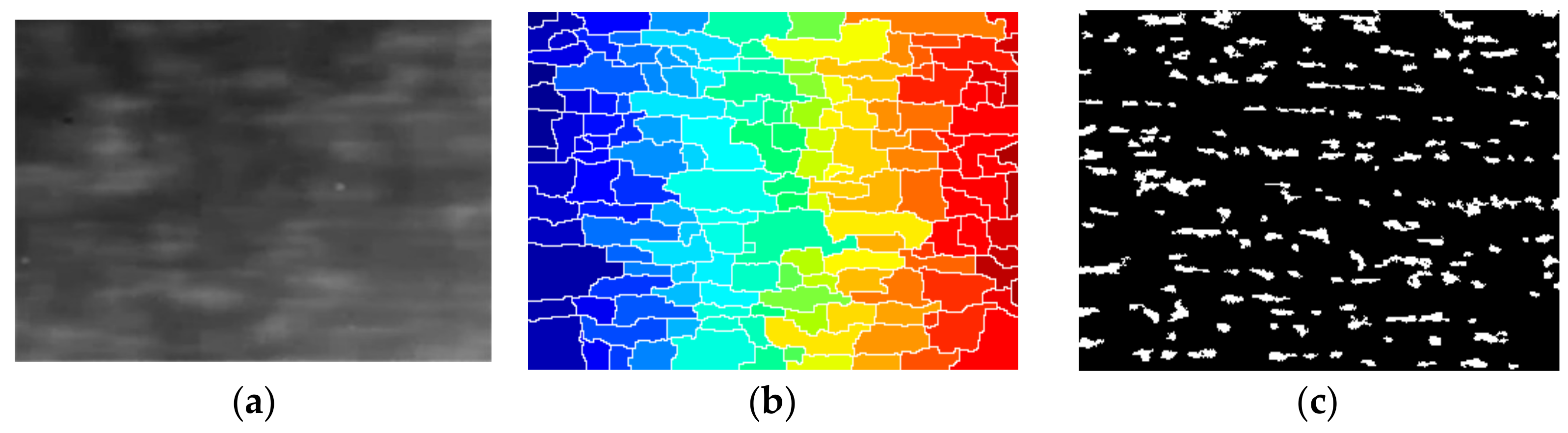
There are many crests and troughs in the sea clutter, and the brightness of the crests is usually higher than that of the troughs. In this paper, the crests and troughs are regarded as the texture of the sea clutter image, and the moving direction of sea clutter is extracted by applying the Watershed transform and the Radon transform in turn. In Figure 2, the Watershed transform segments the sea clutter image into many regions, as shown in Figure 2a, and then separates the troughs from the crests in Figure 2c.

Afterwards, the major axis directions of all troughs in the sea clutter image are counted, and they are exactly perpendicular to the motion direction. In fact, there are two directions perpendicular to the major axis that are opposite each other. Extract the major axis and minor axis of the troughs, and the former is discriminated from the latter based on the common sense that the former is longer than the latter. The average direction $\widehat{\theta }$ of the major axis ${\theta }_i$ of each trough is the motion direction of sea clutter.

$$\widehat{\theta }=\frac{1}{M}{\displaystyle \sum _{i=1}^M{\theta }_i}$$

(2)

where $M$ is the number of troughs, and the major axis direction ${\theta }_i$ is defined as the angle between the major axis and the horizontal line.

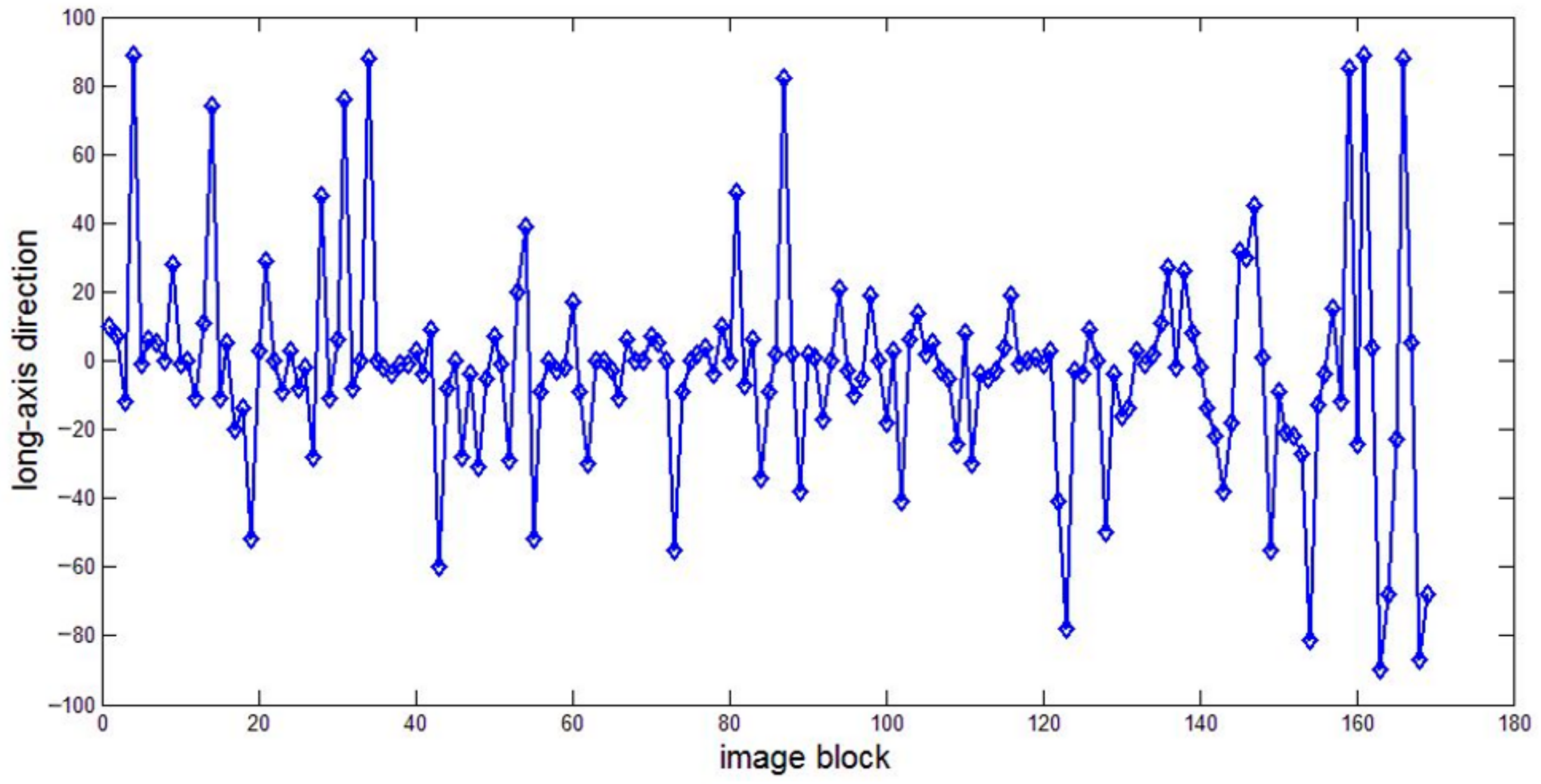
For the infrared sea clutter image shown in Figure 2a, there are more than one hundred and sixty troughs, and their major axis directions are shown in Figure 3. Most major axis directions are concentrated at $0°$, and only a few directions are at $90°$ or $45°$. Therefore, the average direction of the infrared sea clutter image is statistically $0°$. The sea clutter moves from top to bottom or from bottom to top, and the spatial serial data could be selected along this movement direction.

Because the sea clutter propagates in the spatial-temporal domain, the spatial sequence data could accordingly represent the undulatory motion of the seawater. The pixel intensity along the determined motion direction in a static image is the spatial serial data $x_s\left(n,i\right)$. If the sea clutter is dynamic in the space domain, the appropriate delay time and embedded dimension can be used to reconstruct its phase space, and the phase point is expressed as

$$Y_s\left(n,i\right)=\left\{x\left(n,i\right),x\left(n,i+{\tau }_s\right),\cdots ,x\left(n,i+\left(m_s-1\right){\tau }_s\right)\right\}$$

(3)

where ${\tau }_s$ and $m_s$ are the delay time and the embedded dimension of the spatial phase space, respectively.

2.3. Dynamical Parameter Calculation

Seawater particles vibrate periodically or quasi-periodically near their equilibrium position under the action of gravity. Meanwhile, the particles near the vibrating particles also fluctuate due to the continuity of the seawater fluid, and the vibration would spread farther.

For the delay time ${\tau }_t$ in the temporal phase space and the delay time ${\tau }_s$ in spatial phase space, they could be estimated and calculated using the autocorrelation functions of the time data serial and space data serial, respectively. For convenience of description, the time serial data $x_t\left(n,i\right)$ and the space serial data $x_s\left(n,i\right)$ are uniformly abbreviated as $x(n,i)$, and the temporal phase point $y_t(n,i)$ and the spatial phase point $y_s(n,i)$ are also abbreviated as $y(n,i)$. The autocorrelation function of serial data is defined as

$$R\left(\tau \right)=\frac{1}{N}{\displaystyle \sum _{i=1}^{N-1}x\left(i\right)x\left(i+\tau \right)}$$

(4)

where $N$ is the length of the serial data. In general, the autocorrelation function $R\left(\tau \right)$ is a monotonically decreasing function. If it is an aperiodic function, it reaches its maximum value when the delay time $\tau$ is zero. When $R\left(\tau \right)$ decreases to $\left(1-\frac{1}{e}\right)$ of the maximum, the corresponding value $\tau$ is the delay time ${\tau }_t$ in the temporal phase space or the delay time ${\tau }_s$ in the spatial phase space.

Similarly, the embedded dimensions $m_t$ and $m_s$ in the time domain and the space domain are uniformly abbreviated as $m$. The embedded dimension is defined as the minimum dimension required to recover the performance of the original nonlinear dynamic system. When the embedded dimension increases by one, the relative change of the distance between the two adjacent phase points is as follows:

$$a\left(i,m\right)=\frac{x\left(i+\tau m\right)-x^{NN}\left(i+\tau m\right)}{‖Y_m\left(i\right)-Y_m^{NN}\left(i\right)‖}$$

(5)

where $Y_m^{NN}\left(i\right)$ is the nearest phase point to the phase point $Y_m\left(i\right)$ in the $m$-dimensional phase space, $x\left(i+\tau m\right)$ is an element of the phase point, and $‖\cdot ‖$ is the Euclidean norm.

In order to avoid the randomness of distance change caused by only one element, all elements of the phase points in the $m$ dimensional phase space are averaged as

$$E\left(m\right)=\frac{1}{N-m\tau }{\displaystyle \sum _{i=1}^{N-m\tau }a\left(i,m\right)}$$

(6)

When the serial data $x\left(i\right)$ increases from the $m$-dimension to the $\left(m+1\right)$ dimension, the change in distance between the two adjacent points is expressed as

$$E_1\left(m\right)=\frac{E\left(m+1\right)}{E\left(m\right)}$$

(7)

In the dynamical serial data, when $m$ is greater than a certain value $m_0$, $E_1\left(m\right)$ does not change, and the embedded dimension $m$ is defined as $\left(m_0+1\right)$. On the contrary, if the serial data is not dynamic, $E_1\left(m\right)$ would not be saturated. Therefore, the embedded dimension $m$ is an important index to determine whether the serial data is dynamical or not.

Moreover, the associated dimension is also a significant parameter to determine whether the serial data is dynamical or not. It usually increases with the increase in the embedded dimension $m$. For dynamical serial data, when it increases to a certain extent, it becomes saturated. Conversely, if the serial data is random, the correlation dimension would not be saturated. The relevant dimension $D$ is denoted by

$$D=\underset{r\to 0}{\lim }\frac{\ln C\left(r\right)}{\ln r}$$

(8)

where $C\left(r\right)$ is the correlation integral function in the reconstructed phase space $Y(n,i)$ and is denoted as

$$C\left(r\right)=\frac{1}{N\left(N-1\right)}{\displaystyle \sum _{p=1,p\ne q}^N{\displaystyle \sum _{q=1}^{N}H\left(\left(r-‖Y\left(p\right)-Y\left(q\right)‖\right)\right)}}$$

(9)

where $H$ is the Heaviside step function. For the saturated curve of the $D$ function, the correlation dimension is the slope of a straight line that can be fitted by the least square algorithm.

3. Spatiotemporal Dynamics Reconstruction

The property of sea clutter propagation in the spatial-temporal domain makes it possible to reconstruct and estimate the sea clutter through the inherent dynamics model shown in Figure 4. Figure 4a is the framework of the proposed algorithm. Firstly, the infrared sea clutter data is normalized to the original serial data. Then, the temporal dynamics reconstruction function and the spatial dynamics reconstruction function are built based on these extracted dynamical parameters from the original serial data. Afterwards, the space-time coupling coefficient and the spatiotemporal dynamics reconstruction function are estimated using RBF-ANN to estimate the sea clutter. Finally, the sea clutter is suppressed by subtracting the estimated image from the original image, and then the target is detected in the suppressed image. To make the model easier to understand, Figure 4b simply shows the directions of the temporal domain $n$ and the spatial domain $i$ in phase space.

3.1. Intrinsic Dynamics Model

For the dynamical time serial data, the phase trajectory could be acquired by reconstructing the corresponding dynamical phase space. The phase point propagates along the phase trajectory and is expressed as

$$Y_t\left(n+1,i\right)=F_t\left\{Y_t\left(n,i\right)\right\}$$

(10)

where $Y_t\left(n,i\right)$ is the phase point in the time-phase space. Formula (10) could be described by the sea clutter serial data as

$$\left\{x\left(n+1,i\right),\cdots ,x\left(n+\left(m_t-1\right){\tau }_t+1,i\right)\right\}=F_t\left\{x\left(n,i\right),\cdots ,x\left(n+\left(m_t-1\right){\tau }_t,i\right)\right\}$$

(11)

Therefore, the intensity $x\left(n+\left(m_t-1\right){\tau }_t+1,i\right)$ would be related to the time serial data and expressed as

$${\widehat{x}}_t\left(n+\left(m_t-1\right){\tau }_t+1,i\right)=f_t\left\{x_t\left(n,i\right)\right\}$$

(12)

Formula (12) shows that the intensity of the sea clutter image can be predicted and estimated using serial data from the phase space in the temporal domain.

In the same way, the space phase trajectory can be similarly acquired by reconstructing the corresponding dynamical phase space, and the phase point could be denoted as

$$Y_s\left(n,\left(i+1\right)\right)=F_s\left\{Y_s\left(n,i\right)\right\}$$

(13)

where $Y_s\left(n,i\right)$ is the phase point in the spatial phase space and is described by the space serial data as

$$\left\{x\left(n,i+1\right),\cdots ,x\left(n,i+\left(m_s-1\right){\tau }_s+1\right)\right\}=F_s\left\{x\left(n,i\right),\cdots ,x\left(n,i+\left(m_s-1\right){\tau }_s\right)\right\}$$

(14)

Therefore, the intensity $x\left(n,i+\left(m_s-1\right){\tau }_s+1\right)$ could be estimated using the space serial data as

$${\widehat{x}}_s\left(n,i+\left(m_s-1\right){\tau }_s+1\right) =f_s\left(x_s\left(n,i\right)\right)$$

(15)

If the sea clutter image shows dynamical properties in both the spatial domain and the temporal domain, they could be simultaneously estimated by using both the temporal dynamical phase space and the spatial dynamical phase space. Therefore, the intensity of the sea clutter image could be jointly predicted by the temporal serial data and the spatial serial data as [29]

$$\widehat{x}\left(n+\left(m_t-1\right){\tau }_t+1,i+\left(m_s-1\right){\tau }_s+1\right) =\epsilon f_s\left(x_s\left(n,i\right)\right)+\left(1-\epsilon \right)f_t\left(x_t\left(n,i\right)\right)$$

(16)

where $\epsilon$ is a non-negative parameter that describes the coupling strength between the spatial dynamical function and the temporal dynamical function.

3.2. Neural Network-Based Function Estimation

Generally, the spatial dynamical function $f_s\left(x_s\left(n,i\right)\right)$ and the temporal dynamical function $f_t\left\{x_t\left(n,i\right)\right\}$ are nonlinear and implicit functions of the serial data $x_s\left(n,i\right)$ and $x_t\left(n,i\right)$, respectively. Therefore, it is essential to estimate these functions in order to reconstruct the intrinsic dynamical model of sea clutter. It is very important to accurately solve the analytical expression of these functions from a large amount of sea clutter data. An artificial neural network (ANN) is good at processing such serial data with definite non-linear regularity, which is learned by using multiple dominant functions to approximate the inherent correlation of serial data [15].

Because the radial basis function (RBF) based on ANN is good at dealing with small samples, it is adopted in this paper to learn the nonlinear and implicit function of serial data $x_s\left(n,i\right)$ and $x_t\left(n,i\right)$, and its structure is shown in Figure 5. ${\widehat{x}}_t\left(n+\left(m_t-1\right){\tau }_t+1,i+\left(m_s-1\right){\tau }_s+1\right)$ and ${\widehat{x}}_s\left(n+\left(m_t-1\right){\tau }_t+1,i+\left(m_s-1\right){\tau }_s+1\right)$ are predicted by RBF ANN in the temporal and spatial domains, respectively, and then $\widehat{x}\left(n+\left(m_t-1\right){\tau }_t+1,i+\left(m_s-1\right){\tau }_s+1\right)$ is jointly estimated in the spatiotemporal domain.

RBF is a three-layer feedforward network, and its diagram is shown in Figure 6. The transfer function of the network node in the hidden layer is a radial basis function that could generate a local response to the input. The hidden layer converts the input data vector in low-dimensional mode into high-dimensional space, so that the linearly inseparable problem in low-dimensional space could be linearly separable in high-dimensional space.

The Gaussian function is introduced in this paper as a radial basis function and denoted as

$${\phi }_i\left(x\right)=\exp \left(-\frac{‖x-c_i‖}{2{\sigma }_i^2}\right)$$

(17)

where $c_i$ and ${\sigma }_i^2$ are the center and the size of the $i^{th}$ node, respectively.

The output of the $k^{th}$ output node linearly combines the output of the nodes in the hidden layer as

$$Z_k={\displaystyle \sum _i{\omega }_{k,i}}{\phi }_i-b_k$$

(18)

where $b_k$ is the bias of the $k^{th}$ output node, and ${\omega }_{k,i}$ is the weight between ${\phi }_i$ and $Z_{\mathrm{k}}$.

There are three unknown parameters in Formulas (17) and (18), namely, the center $c_i$, size ${\sigma }_i^2$, and weight ${\omega }_{k,i}$, that are learned during the RBF neural network training. This paper introduces a method called self-organizing center selection to solve these parameters [28]. After the spatial dynamical function $f_s\left(x_s\left(n,i\right)\right)$, the temporal dynamical function $f_t\left\{x_t\left(n,i\right)\right\}$, and the coupling parameter $\epsilon$ are estimated, the sea clutter would be estimated using Formula (16). In the experiment, the first half of the infrared image sequence is used to train RBF ANN, and the latter part is applied to verify the performance of the infrared sea clutter suppression.

4. Sea Clutter Suppression and Target Detection

The sea clutter could be accurately predicted and estimated through the spatial-temporal dynamical neural network, so the difference between the estimated signal and the original signal would consequently fluctuate around zero with a higher probability. On the contrary, it is difficult to use the dynamical neural network to estimate the target signal because it usually fails to abide by the spatial-temporal dynamics of the sea clutter, and the difference between the estimated signal and the original signal would be larger compared with that of the sea clutter. Therefore, the sea clutter could be suppressed, and the target signal could be enhanced by the difference between the estimated signal and the original signal.

$$\tilde{x}\left(n,m\right)=x\left(n,m\right)-\widehat{x}\left(n,m\right)$$

(19)

Generally, the differential image might be subordinated to Gaussian white noise, and the target could be detected with a higher probability by the criterion of the constant false alarm rate (CFAR). In addition, the trajectory of the target is continuous and consistent, and it appears in the neighboring region at consecutive images with maximum probability since it moves continuously. Therefore, the target would be declared by M/N logic, that is, if there are more than M measurement values in N consecutive images, the measurement value is assumed to be a potential target; otherwise, it is a false alarm.

5. Experimental Results and Analysis

In the experiments, the sea clutter image sequences are included to verify whether the sea clutter image has dynamical properties in the space and time domains, and then five algorithms are used to evaluate and compare their performances, namely, top-hat, the estimation based on the spatial dynamics, the estimation based on the temporal dynamics, the spatial-temporal domain joint filtering [1], and the proposed algorithm. It is noteworthy that this experiment mainly focuses on the results obtained after introducing spatial dynamics into conventional temporal dynamics methods. Meanwhile, the critical issue of this paper is how to suppress the fluctuating sea clutter in the spatiotemporal domain. Therefore, in addition to other spatial methods that are good at dealing with static background, the top-hat filter [7,8,9] is discussed as the baseline method.

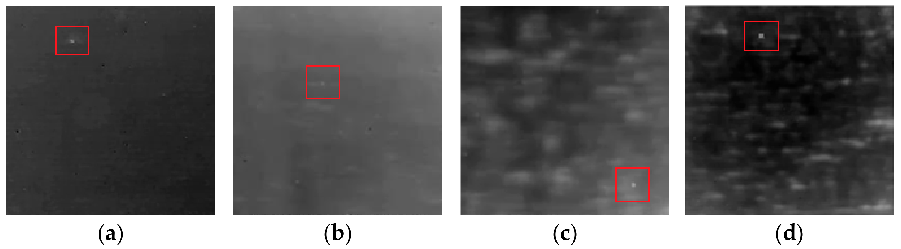
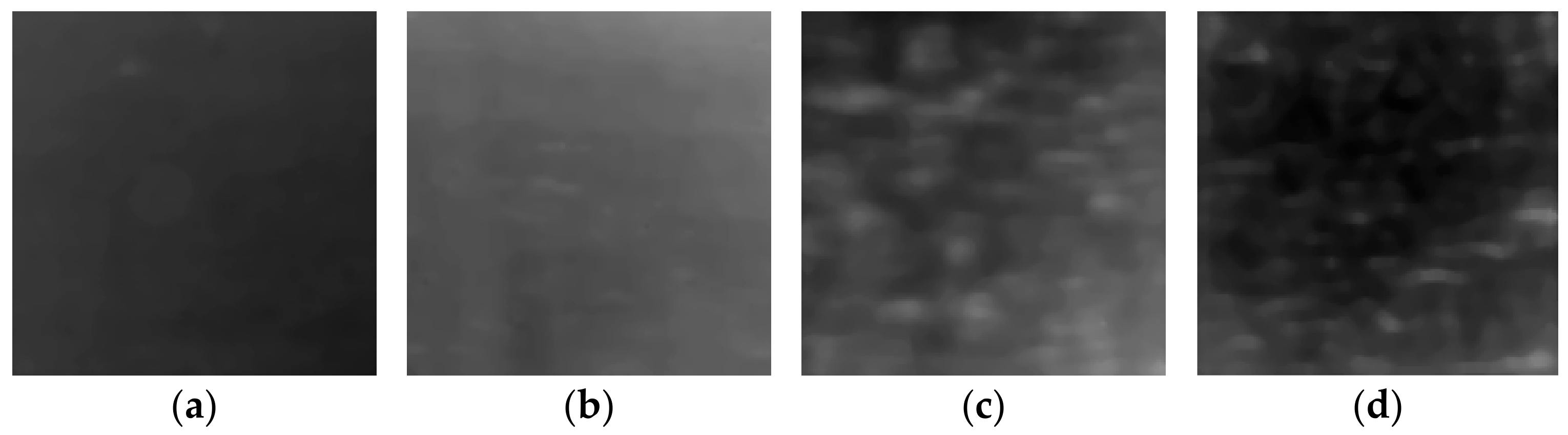
Figure 7 shows four infrared sea clutter image sequences with various fluctuations in the experiments, and the small targets are highlighted with red rectangles. Each infrared sequence has 50 images. The size of each image is 256 × 256 pixels, and the depth is 8 bits. In Figure 7a–d, the fluctuation of sea clutter becomes stronger. There is little fluctuation in Figure 7a, the sea clutter fluctuates weakly in Figure 7b, and the crests and troughs are obvious in Figure 7c,d. Their signals-to-clutter ratios (SCRs) are 2.94, 2.52, 1.58, and 0.88, respectively. Although the target in Figure 7d is brighter than in Figure 7b, the former’s SCR is smaller than that of the latter.

5.1. Spatiotemporal Dynamics Test

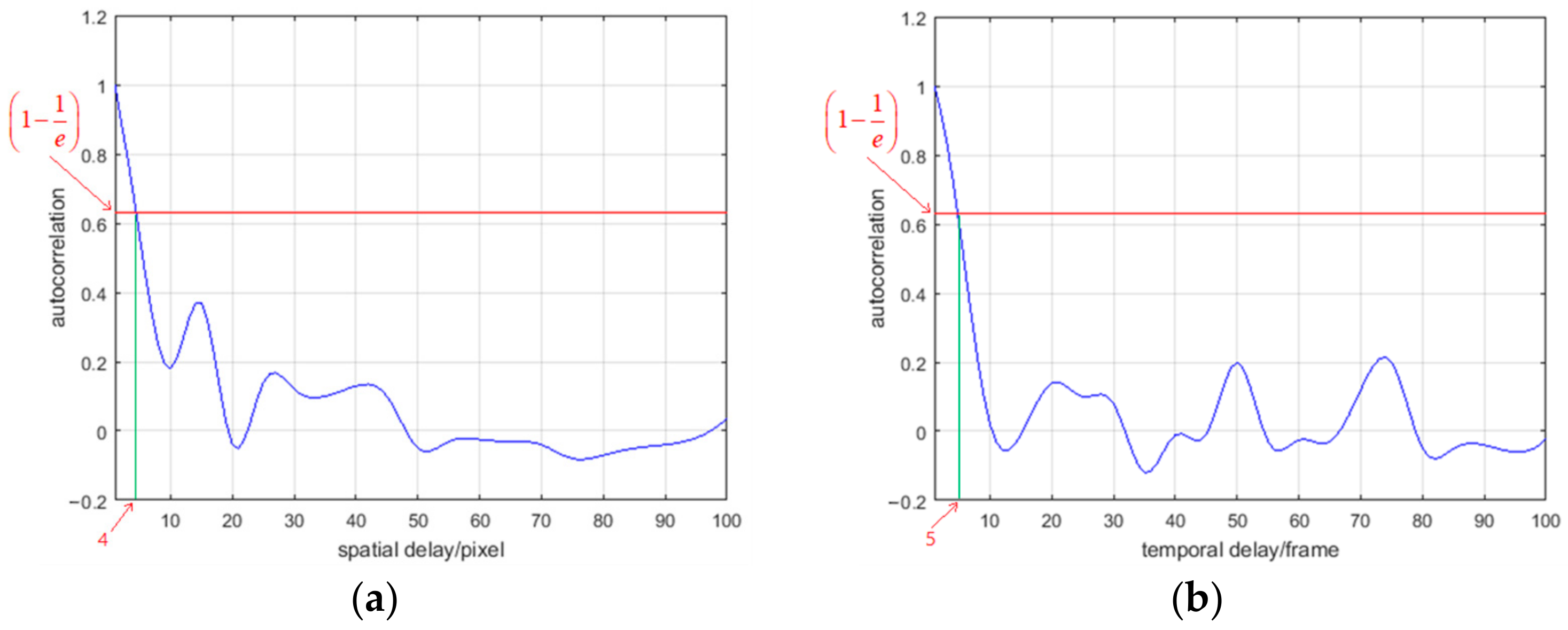
To simplify the description of the experiment, only the sea clutter image in Figure 7d is used to verify its dynamics in the spatiotemporal domain. The spatial autocorrelation function and the temporal autocorrelation function are shown in Figure 8. The spatial delay time ${\tau }_s$ and the temporal delay time ${\tau }_t$ are 4 pixels and 5 frames, respectively.

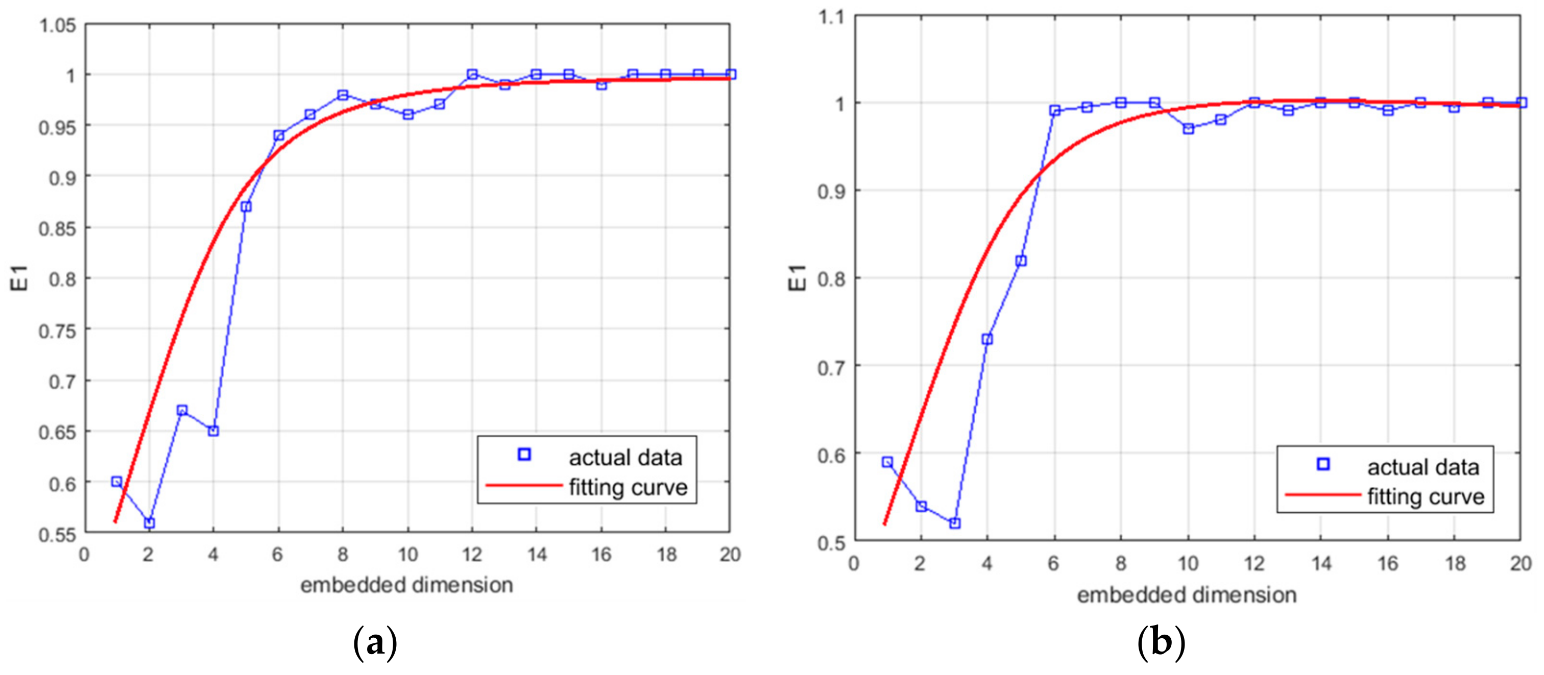
Figure 9 shows the function $E_1\left(m\right)$ on the spatial embedded dimension and the temporal embedded dimension. $E_1\left(m\right)$ and the fitting curve increase with the increase in the embedded dimension. In the early stages of growth, the growth rate of the curve, namely the slope, is very large. When the embedded dimension increases to a certain extent, the growth rate will slow down to zero. Therefore, the actual embedded dimension is determined when the growth rate is lower than 10% for the first time. In Figure 9, the spatial embedded dimension and the temporal embedded dimension are equal to 7 and 6, respectively.

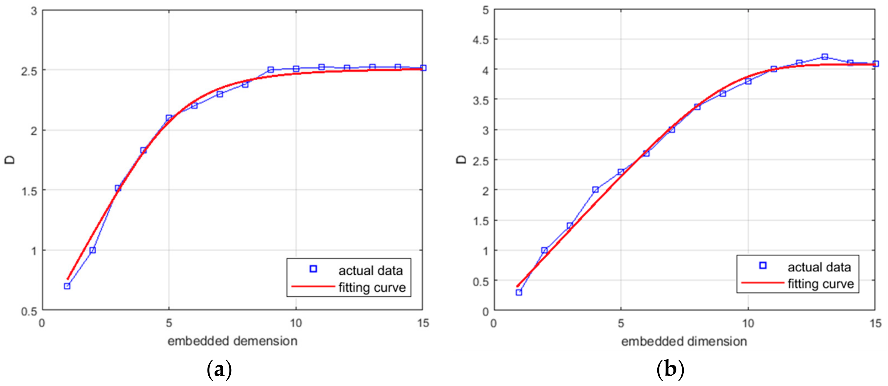
Figure 10 shows the correlation dimension $D$ on the spatial embedded dimension and the temporal embedded dimension. The correlation dimension $D$ and the fitting curve increase with the increase in the embedded dimension. The spatial embedded dimension and the temporal embedded dimension are equal to 10 and 12, respectively. After correction and fitting, the spatial correlation dimension and the temporal correlation dimension are equal to 0.40 and 0.45, respectively, and they indicate that the infrared sea clutter image is dynamic in the spatiotemporal domain.

The infrared images of sea clutter with a variety of undulations are also tested, and the sea clutter is not dynamic when it fluctuates too strongly or too weakly. The sea clutter squints more towards random and periodic signals when it undulates too strongly or too weakly. For example, it is difficult for the watershed transform to segment the troughs of the sea clutter that is a random signal with a stationary mean when the sea wave is homogeneous.

The four reconstructed images by the proposed algorithm are illustrated in Figure 11. Most of the sea clutter in Figure 11a–c has been reconstructed, while the targets have not been estimated. It is beneficial to improve the signal-to-noise ratio of the target in the image after sea clutter suppression. In Figure 11d, some small undulating waves of the sea clutter could not be effectively reconstructed due to their small size.

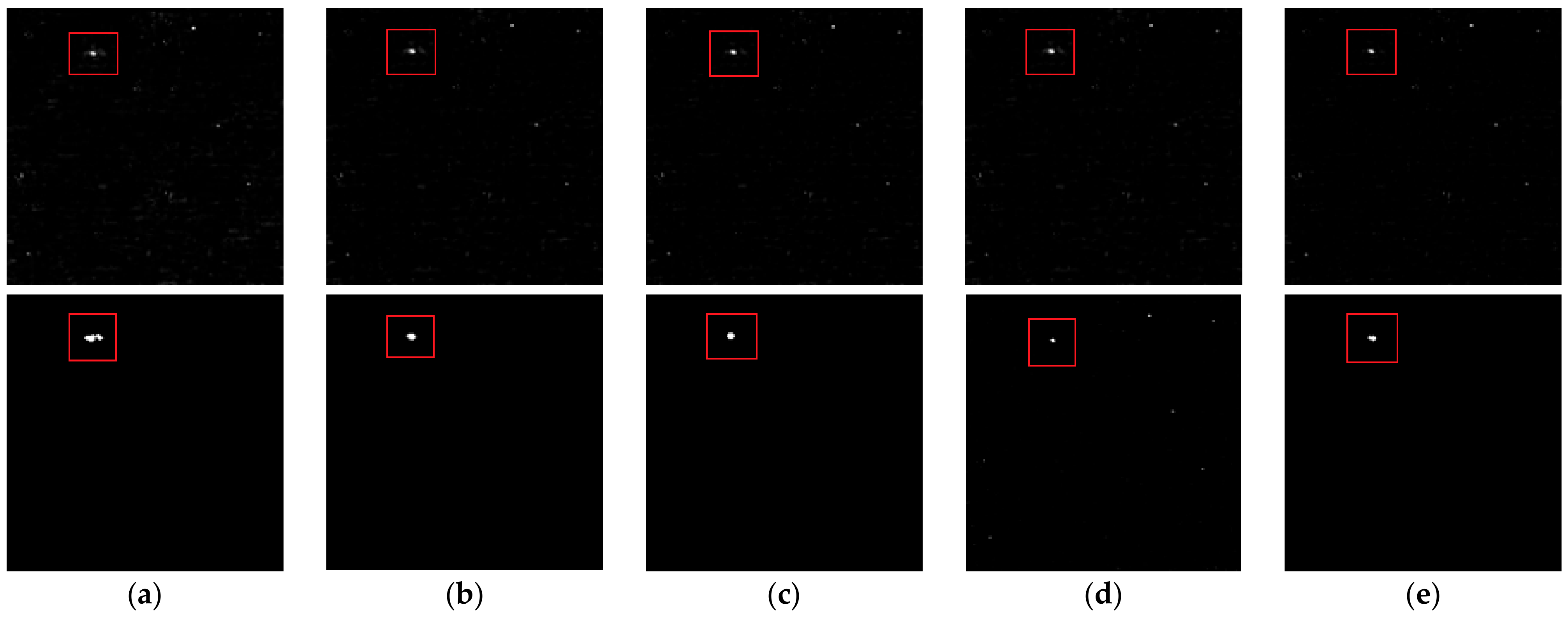
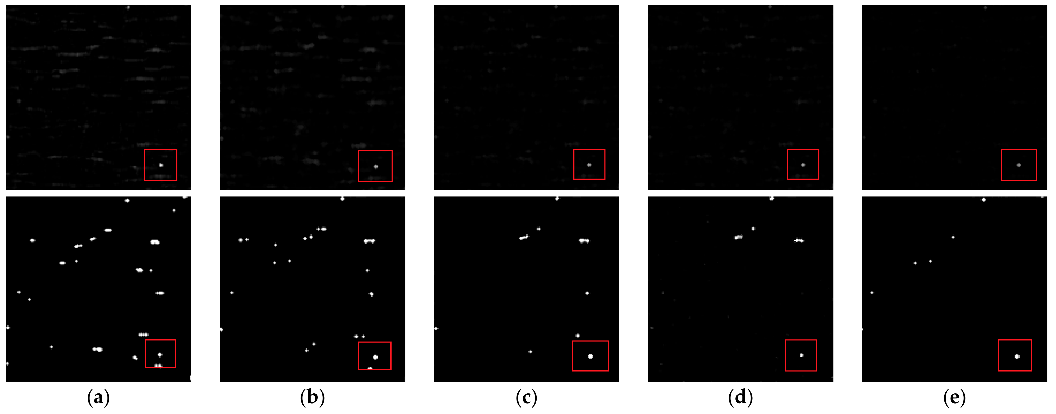
5.2. Sea Clutter Suppression Performance

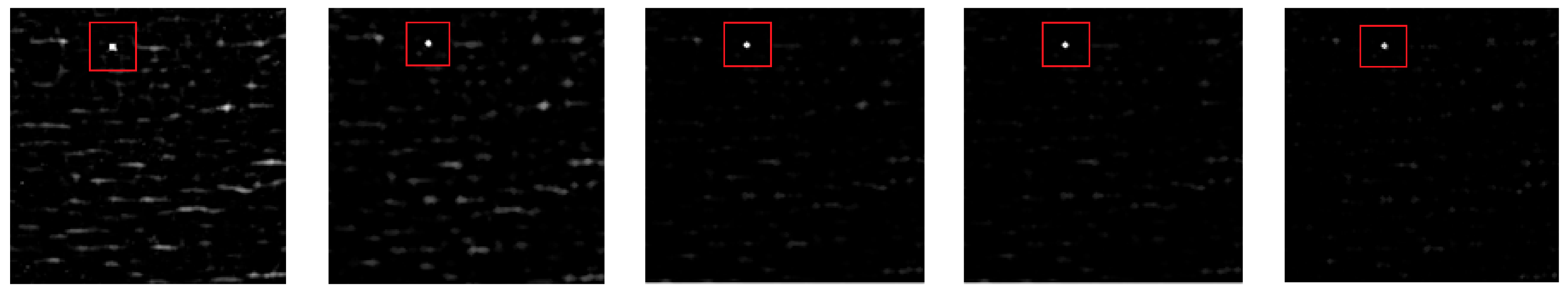
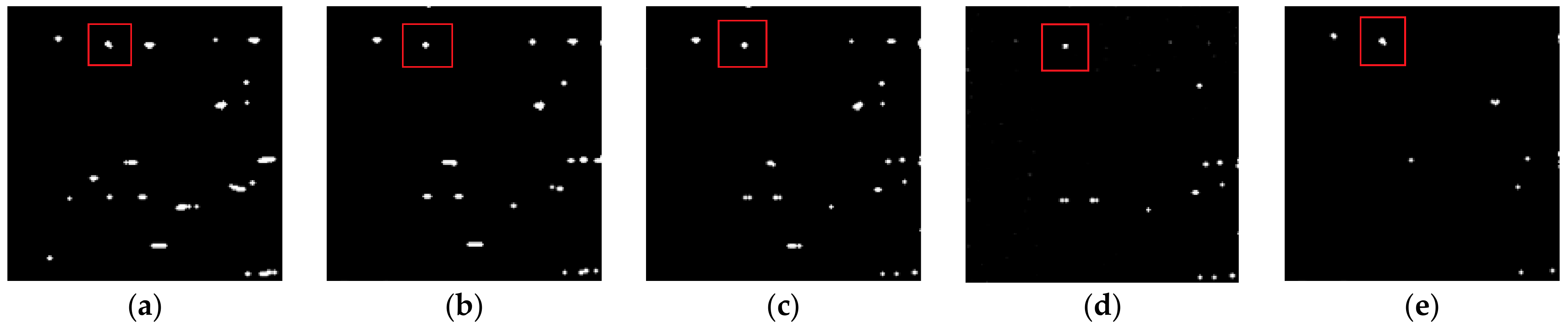
In addition, for these four sea clutter image sequences with various fluctuations, the residual images and the detected images are shown in turn in Figure 12, Figure 13 and Figure 14, and the first row and the second row are the residual images and the detected images, respectively. The small target in each image is heighted with red box. The structure element of the top-hat algorithm is 5 × 5 pixels. In the case of smooth sea clutter, shown in Figure 12, these five algorithms could accurately estimate the sea clutter and effectively detect the small target.

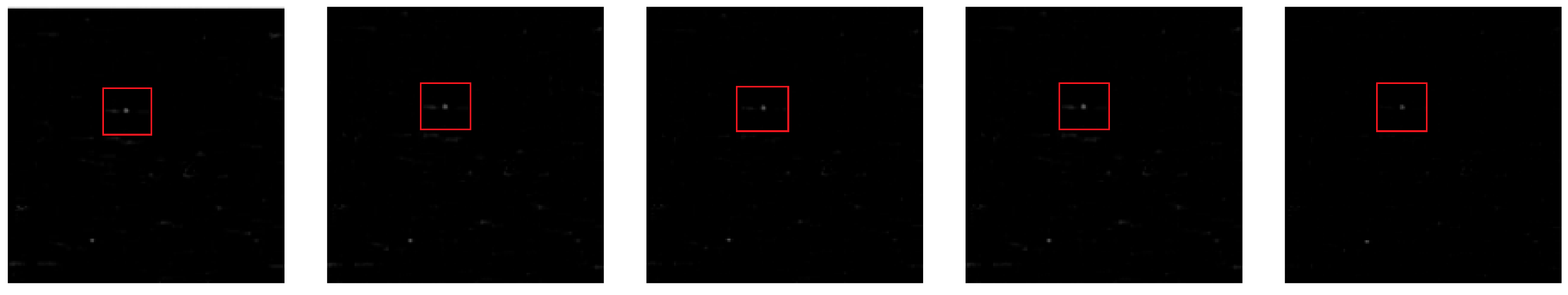
In the case of weak fluctuation, as shown in Figure 13, the residual image processed by top-hat has some big errors at the edge of the crest, and the binary image also has false alarms consistent with the wave direction. Instead, the residual images processed by the other four algorithms have no obvious remnants, and the target was also detected effectively. Moreover, the residual in the proposed algorithm is a little more serious than that of the other three dynamical algorithms.

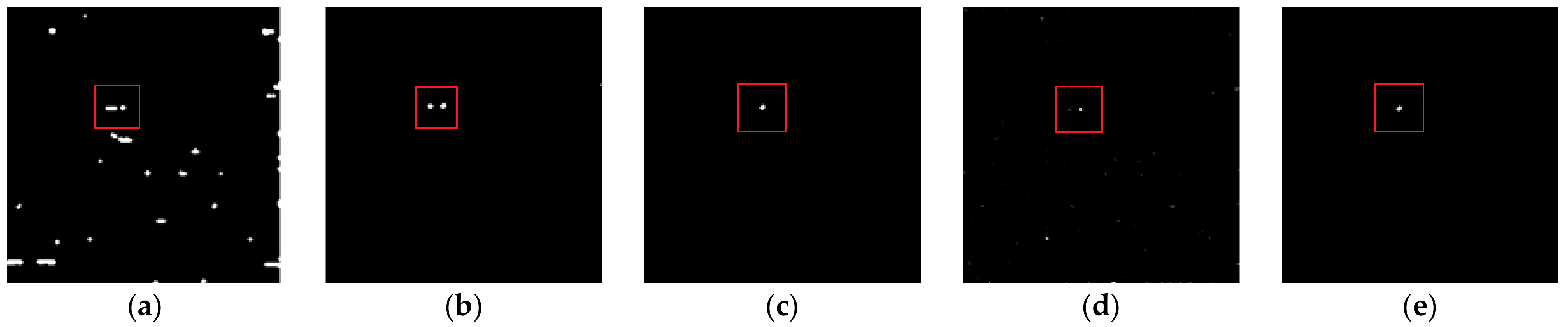
In the moderate fluctuation shown in Figure 14, there are a large number of crests and troughs in the glittering sea clutter. The residual images processed by top-hat and spatial dynamics have more remnants and false alarms than those processed by the temporal dynamics, spatio-temporal filter, and proposed algorithm.

In the case of strong fluctuations, as shown in Figure 15, the residual images processed by top-hat and spatial dynamics have a large number of remnants and false alarms because they cannot effectively estimate the crest and trough. However, the proposed algorithm has achieved the best performance with fewer remnants and false alarms, and its target detection performance is also the most prominent.

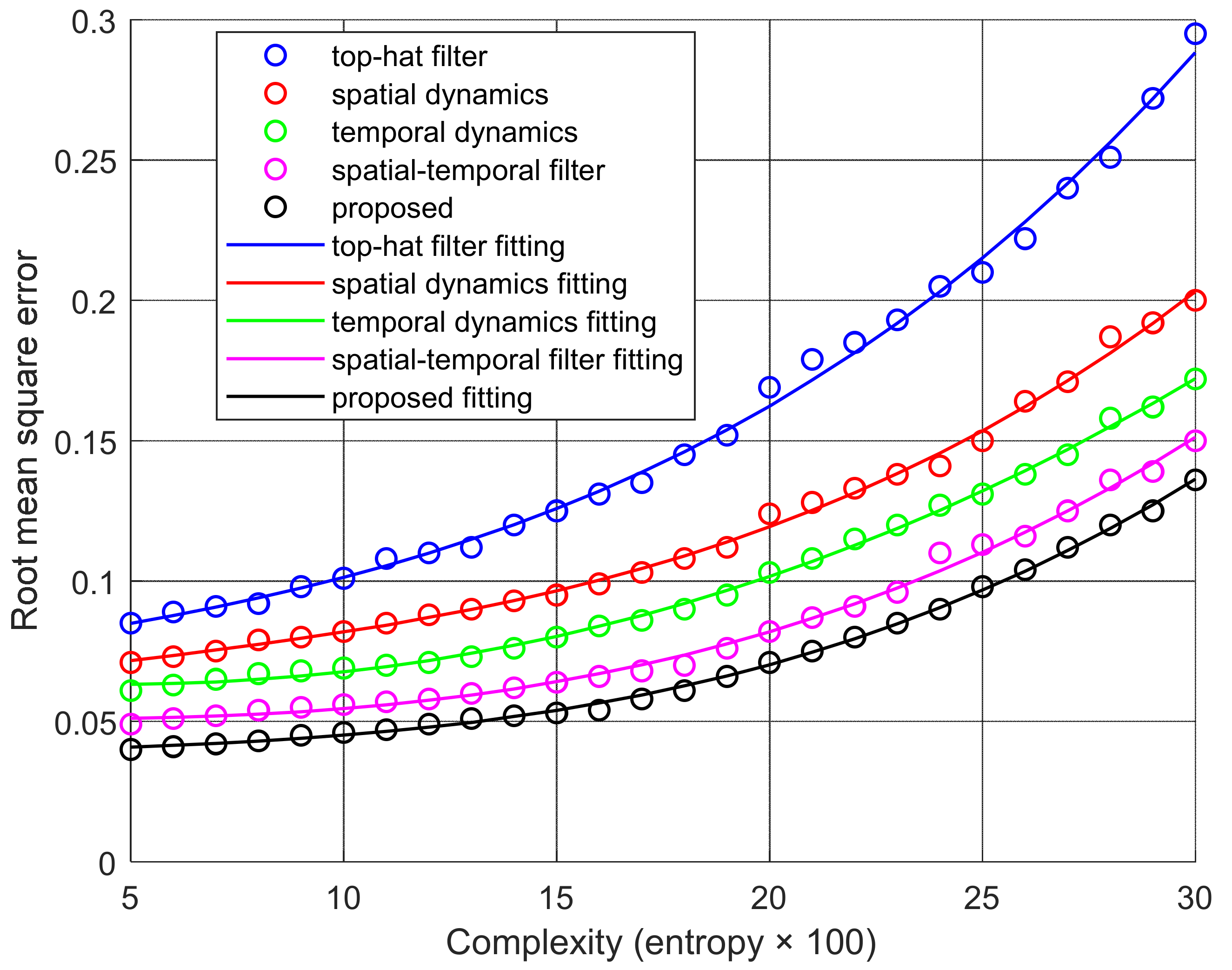
The estimation error under various fluctuations is shown in Figure 16, in which the entropy of the whole image is adopted to represent the degree of sea clutter fluctuation. The estimation error is normalized to 0.3, and it increases with the increase in fluctuations in evidence. The error of the proposed algorithm is the smallest, and it is only half that of spatial dynamics when the complexity is 5 to 20. The entropies of the four infrared image sequences are 0.08, 0.14, 0.22, and 0.3, and their SCRs are 2.94, 2.52, 1.58, and 0.88, respectively.

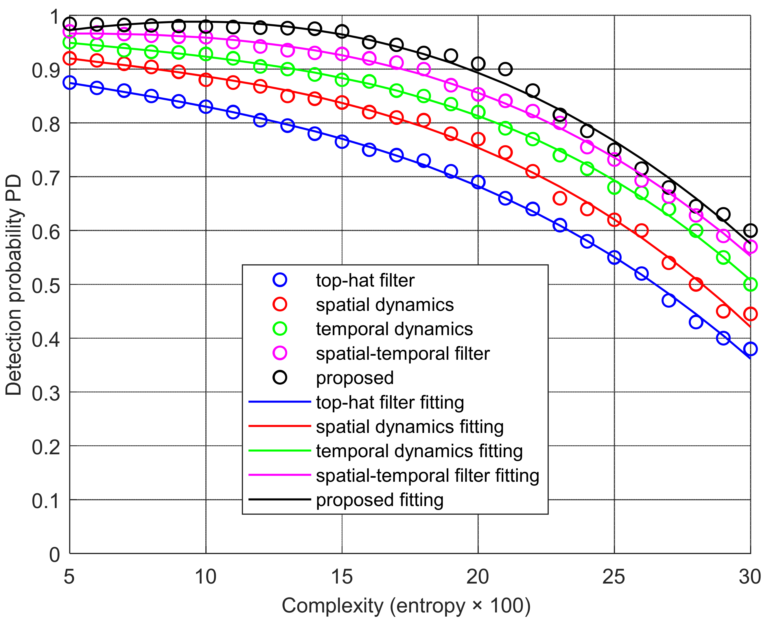
The target detection probability at various fluctuations is shown in Figure 17, where the constant false alarm rate is 0.01. The proposed algorithm achieves the highest detection probability. When the sea clutter is dynamic in the spatiotemporal domain, its performance is improved by 20%. It is worth noting that the target detection performances of these five algorithms would decline rapidly when the fluctuation was very severe.

The above experiments were carried out using a personal computer with an i5 Dual-Core CPU of 3.2 GHz and a memory of 16 GB. The program codes were written in MATLAB R2020a. The computational complexity of each algorithm in the four infrared image sequences is shown in

Table 1. The comparison of the computational complexity of each algorithm.

		Methods	Top-Hat	Spatio-Temporal Filter	Temporal Dynamics	Spatial Dynamics	Proposed Algorithm
	Computational Complexity (Second)
Images
Smooth			0.53	1.67	3.37	3.22	5.77
Weak			0.57	1.71	3.24	3.44	5.81
Moderate			0.57	1.79	3.53	3.39	5.92
Strong			0.58	1.80	3.67	3.50	6.02

. The average time spent by the top-hat algorithm is the least because it only suppresses sea clutter in the spatial domain without complex operations. The temporal domain dynamics algorithm and the spatial domain dynamics algorithm take a moderate amount of time because they only involve the construction of a single dimension of the image sequence. However, the proposed algorithm would take more time.

6. Conclusions

This paper proposes a method of detecting small targets in sea clutter infrared images based on spatiotemporal dynamics analysis. Firstly, the temporal dynamics reconstruction function and the spatial dynamics reconstruction function are built using the extracted dynamical parameters. Secondly, the space-time coupling coefficient and the spatiotemporal dynamics reconstruction function are estimated by means of RBF ANN to reconstruct the propagation regularity of the moving sea clutter. Finally, the sea clutter is suppressed by subtracting the estimated image from the original image, and then the target is detected in the suppressed image by the CFAR criteria. The experimental results of various fluctuations in the infrared sea clutter image sequence show that the proposed algorithm based on spatiotemporal dynamics could reduce the sea clutter suppression error by 10% and improve the small target detection probability by 20% under certain fluctuations.

In addition to its high computational complexity, the main limitation of the proposed method is that the infrared detector would need to be altered because the temporal dynamical reconstruction requires that the pixels be aligned in the image sequence. Future work will focus on reducing complexity and improving viability.