Article

Radiative Effects and Costing Assessment of Arctic Sea Ice Albedo Changes

1
State Key Laboratory of Earth Surface Processes and Resource Ecology, Beijing Normal University, Beijing 100875, China
2
Frontier Science Center for Deep Ocean Multispheres and Earth System and Physical Oceanography Laboratory, Ocean University of China, Qingdao 266100, China
*
Author to whom correspondence should be addressed.
Remote Sens. 2023, 15(4), 970; https://doi.org/10.3390/rs15040970
Submission received: 19 November 2022 / Revised: 2 February 2023 / Accepted: 6 February 2023 / Published: 10 February 2023
(This article belongs to the Special Issue Remote Sensing Monitoring for Arctic Region)

Abstract

:
The rapid loss of Arctic Sea ice cover and thickness diminishes the surface albedo, which increases the ocean’s absorption of solar heat and exacerbates the Arctic amplification effect. According to the most recent research from the Intergovernmental Panel on Climate Change, the Sixth Assessment Report (IPCC, AR6), the extent of summer sea ice is anticipated to decrease below 1 million km2 by the 2050s as a result of the extreme climate. Nevertheless, past and future changes in sea ice albedo radiative forcing and the resulting economic cost remain to be explored in systematic and multi-disciplinary manners. In this study, we first analyze the evolution of Arctic sea ice radiative forcing (SIRF) from 1982 to 2100 using a radiative kernel method based on albedo data from the Polar Pathfinder-Extent (APP-x) and Coupled Model Intercomparison Project 5 (CMIP5). Then, the SIRF is converted to CO2 equivalent emissions via the Dynamic Integrated Model of Climate and Economy (DICE) model. Finally, the associated costs are calculated using the substitute cost method, based on the social cost of carbon to achieve the Paris Agreement targets. The results show that the average Arctic SIRF was −0.75 ± 0.1 W · m 2 between 1982 and 2020, and increased by 0.12   W · m 2 during this period. The SIRF in April–June accounts for nearly 77% of the average annual value, with a maximum absolute value of –3.2 W · m 2 in May. Through model transformation, it is shown that the Arctic SIRF rising leads to global warming comparable to the effect of an increase of 34.5 Gt of CO2 in the atmosphere relative to pre-industrialization, and results in a loss of 24.4–48.8 trillion USD for climate regulation service (CRS). From 2020 to 2100, in the representative concentration pathway (RCP) 8.5, the Arctic SIRF is projected to increase by 0.31   W · m 2 . Combined with the discount rate, the estimated average annual cost over the period ranges from 6.7–13.3 trillion USD. These findings provide a systematic understanding of the radiative effect of Arctic sea ice change on the global climate and the corresponding economic cost.

1. Introduction

Sea ice loss is the primary cause of “Arctic amplification”, which refers to the rate of Arctic warming being three to four times faster than the rest of the globe over the past few decades [1,2,3,4]. The loss of Arctic sea ice is mostly manifested by decreased extent and thickness [5,6,7,8]. Shrinking ice and extending melt seasons [9,10,11] reduce surface albedo [12,13], leading to increased solar absorption at the surface, which amplifies warming and drives more melting. Thus, sea ice plays a cooling role in the Earth’s climate system by regulating the surface energy balance, known as the climate regulation service (CRS) of sea ice [14,15,16]. However, this CRS is deteriorating with sea ice loss, affecting the Arctic ecosystem [17] and exacerbating global climate change impacts. In addition, since climate change carries significant economic impacts on the global economy [18], the loss of sea ice CRS will also have additional economic impacts far beyond the Arctic itself [19].
Any change in sea ice cover strongly affects the climate response through the surface albedo feedback [20,21], and variations in sea ice albedo can be explained by sea ice concentration (SIC), surface air temperature, and melt onset as drivers [13]. As sea ice begins to melt or disappear entirely, darker ocean surfaces absorb more solar radiation [22], and the increase in open water in the Arctic Ocean may have already led to a 50% increase in shortwave absorption since 1979 [23]. The effect of observed changes on the reduction in winter ice growth in 2007 was about 44 cm, with a 10–36 day delay in autumn freeze-up [24]. The positive trend of solar radiation absorption by the ocean in summer in the Arctic is more than twice that of the land, which is the primary radiative feedback mechanism in the Arctic [25]. Graversen and Wang [26] used the community climate system model version 3 (CCSM3) to simulate the feedback effect of Arctic Sea ice albedo, and showed that the amplification of the surface temperature response in the Arctic was about 33%, while the amplification of the global mean surface temperature was about 15%.
Sea ice albedo in the Arctic has shown a significant decreasing trend over the last few decades [13,27,28], and several studies have estimated the radiative impact of this change at regional or global scales [21,29,30,31,32,33]. The transient perturbation of the Earth’s top-of-atmosphere (TOA) energy balance by sea ice albedo changes is known as sea ice radiative forcing (SIRF). Flanner et al. [29] estimated the radiative forcing due to the cryosphere change in the Northern Hemisphere using modelled radiative kernels and a range of model-based and satellite-based surface albedo measurements. They found that the annual mean SIRF is −0.65 W · m 2 and that it had increased by 0.11 W · m 2 between 1979 and 2008. Based on the satellite-retrieved long-term surface albedo product CLARA-A1 (Cloud, Albedo, and Radiation dataset, AVHRR-based, version 1) and the radiative kernel method, Cao et al. [31] calculated that the SIRF is −0.83 W · m 2 , indicating that the reanalysis products of the European Centre for Medium-Range Weather Forecasts Interim Reanalysis (ERA-Interim) and Modern-Era Retrospective Analysis for Research and Applications (MERRA) severely underestimate the interannual variability of SIRF during the melting season (May–August). Pistone et al. [30] directly used the planetary albedo from the Cloud and Earth Radiant Energy System (CERES) product, and estimated the SIRF in the Arctic Ocean (north of 60°N). They found that the change in SIRF due to sea ice loss from 1979 to 2011 was 0.21 W · m 2 , which is twice as large as that estimated by Flanner et al. [29]. Thus, there are significant differences regarding the estimated results, due to the inconsistent selection of albedo data and different estimation methodologies applied [31].
The ice-albedo feedback is a key driver of Arctic climate change and an important uncertainty source of future sea ice projections in coupled climate models [34]. Especially, there is substantial uncertainty about how much ice retreat and associated SIRF changes will occur in the future. According to the IPCC AR6, the projection shows that by the end of the 21st century, the Arctic will be nearly ice-free in September [35,36]. Regardless of the rate of Arctic sea ice decline, a direct consequence of ice-free sea conditions is the elimination of the SIRF, with the ocean absorbing more energy and generating a self-reinforcing warming mechanism. Pistone et al. [37] estimated that the solar energy would increase in the worst-case scenario of the complete disappearance of Arctic sea ice throughout the sunlit period of the year, obtaining associated global radiative forcing of 0.71 W · m 2 relative to the 1979 baseline state. The result is similar to the radiative forcing of a complete removal of sea ice (i.e., 0.7 W · m 2 ) [38]. If air temperature continues to increase, ice-free conditions will become the norm for a portion of each summer in the future, and this will gradually extend into spring and autumn [39,40]. However, future Arctic SIRF changes have not been estimated using radiative kernel method so far but with the relationship between sea ice extent and albedo.
In recent years, the economic costs of Arctic climate and cryosphere changes have also received more attention. Euskirchen et al. [41] estimated that the annual cost due to the declining albedo of sea ice and snow and methane emissions from permafrost is expected to be 7.5–91.3 trillion USD by 2100. Badina and Pankratov [42] projected that the cumulative cost of climate change in the Arctic zone of the Russian Federation during 2020–2050 will be more than 111 billion USD (in 2020 prices). Yumashev et al. [43] assessed the nonlinear transitions in Arctic feedback and global climate and economic impacts under various climate mitigation scenarios. They noted that the increased permafrost feedback and weakened albedo feedback could result in significant increases in the mean discounted economic effect of climate change. Moreover, other integrated economic-climate models have been created to analyze climate change and its economic implications in an integrated manner, with the Dynamic Integrated Model of Climate and Economy (DICE) model [44] being one of the most extensively used integrated models. For instance, Nordhaus [45] have applied this model to assess the economic impacts of the melting of the Greenland ice sheet. However, the economic cost of the deterioration in the climate regulating services of Arctic sea ice still needs to be conducted.
This study intends to investigate the effect of Arctic sea ice albedo on the global energy balance based on the concept of CRS, and to estimate the past and future global economic cost of SIRF change. Initially, we estimate the SIRF for 1982–2100 using a radiative kernel method based on albedo data from the Polar Pathfinder-Extent (APP-x) and Coupled Model Intercomparison Project 5 (CMIP5). Using the DICE model, we then convert SIRF to carbon dioxide equivalent emissions. Finally, we further assessed the economic cost of the deterioration in the climate regulating services of Arctic sea ice using a substitute cost method. In addition, we also compared the effects of different albedo data and radiative kernels on the calculations, with the aim of more accurately understanding the contribution of Arctic sea ice albedo to global radiative forcing. This study will provide a systematic understanding of the radiative effects of Arctic sea ice change on the global climate and the associated economic cost.

2. Materials and Methods

To estimate past and future Arctic SIRF changes and the associated economic costs, the radiative kernel method, the DICE model, and substitute cost method are mainly used in the study. Table 1 provides a summary of the datasets utilized in this study.

2.1. Estimating SIRF Using the Radiative Kernel Method

In this study, we use the radiative kernel method from [29,31,33] to calculate the SIRF in the Arctic. Radiative kernel methods were first proposed for estimating water vapor feedback in climate models, were later applied to temperature, vertical decrement rate, and albedo feedback [46], and are now widely used in climate model predictions of global warming and studies on the response to increasing CO2 levels. The radiative kernel method decomposes the feedback into a factor that depends on the radiative transfer algorithm and undisturbed climate state and a second factor generated by the climate response of the feedback variable [46]. The advantage of this method is its high computational efficiency, and the disadvantage is its vulnerability to radiative transfer errors and biases because the kernel technique assumes a linear relationship between radiative response and climate change. Following Flanner et al. [29], we calculated sea ice radiative forcing (SIRF) using the sea ice albedo and radiative kernel. The time (t) dependence of SIRF within a region R (the global region) of area A, composed of gridcell r, is expressed as Equation (1):
SIRF t , R = 1 A R R   I t , r α p α s t , r α c s i t , r d A r
where I t ,   r is the TOA incident solar radiation for each grid, α p α s represents the planetary albedo change due to perturbations in the surface albedo (usually specified as 1%), and the product of the two terms is the radiative kernel, traditionally described as the change in the top atmospheric radiation flux due to the albedo ( F / α ). The α c s i t , r represents the albedo of sea ice minus water. The ocean’s average albedo is about 0.05 to 0.10 [47]. Here, the average albedo of seawater is 0.068 according to a previous report [31]. A(R) is the area of the Earth (510 million km2).
The Arctic ice albedo products from the Extended Advanced Very High-Resolution Radiometer (AVHRR) Polar Pathfinder (APP-x), the Modern-Era Retrospective analysis for Research and Applications version 2 (MERRA-2) and the European Centre for Medium-Range Weather Forecasts reanalysis version 5 (ERA5) were used to calculate the SIRF for the period 1982–2020. The APP-x data products were downloaded from the National Oceanic and Atmospheric Administration (NOAA) of the United States. NASAs Global Modeling and Assimilation Office provides the MERRA2 reanalysis, while the European Centre for Medium-Range Weather Forecasts provides the ERA5. APP-x albedo has a high spatial resolution and has been validated by the Surface Heat Balance of the Arctic Ocean (SHEBA) field experiment [48,49], hence it is utilized to estimate the past SIRF. In addition, albedo data from MERRA2 and ERA5 are used to estimate the SIRF for comparison purposes.
Typically, radiative kernels are generated using base data from global climate model simulations as a function of latitude, longitude, elevation, and month in both all-sky and clear-sky conditions. Here, we used the monthly average of the TOA albedo radiative kernel from three different models: the Community Atmosphere Model of Version 5.0 (CAM5), the Geophysical Fluid Dynamics Laboratory atmospheric model (GFDL); and the HadGEM2-ES climate model (HadGEM2). Details of the albedo and radiative kernel data are shown in Table 1.
Due to the latest CMIP6 not so far outputting sea ice albedo data, the monthly Arctic Sea ice albedo output from the Scenario Model Intercomparison Project of the six CMIP5 models is collected (Table 1). The model outputs are available from https://data.ceda.ac.uk/badc/cmip5/data/cmip5/ (accessed on 19 November 2022). Because many models lack sufficiently large ensembles, only the first ensemble member (r1i1p1f1) of each model is chosen. The future scenarios are based on three Representative Concentration Pathways (RCPs): RCP2.6, RCP4.5, and RCP8.5 [50]. The RCPs are a comprehensive set of concentration and emission scenarios used as input parameters for climate change projection models under the influence of human activities in the 21st century [51]. RCP8.5 is the baseline scenario without government action in climate change policy, RCP4.5 is the climate scenario with government intervention, and RCP2.6 is the scenario with extremely low greenhouse gas concentrations. The sea ice albedo of the CMIP5 models with APP-X were time overlapped for 2006–2020. The mean, mean absolute error (MAE), and root mean square error (RMSE) of the albedo deviation for this period in the area north of 70°N were used to validate the CMIP5s sea ice albedo data.
Since the albedo data from satellite observations and reanalysis include sea ice, seawater, and land, SIC (Table 1) is required to identify sea ice locations. The monthly sea ice concentration is obtained from NSIDC [52], which is derived from the Nimbus-7 Scanning Multichannel Microwave Radiometer (SMMR), the US Defense Meteorological Satellite Program (DMSP) Special Sensor Microwave Imager (SSM/I), and the Special Sensor Microwave Imager/Sounder (SSMIS). The locations where the monthly mean SIC is greater than 0 are identified as masks used to determine sea ice cover.
In this study, all the variables and radiative kernels were re-gridded at a spatial resolution of 25 km using EASE-Grid 2.0 [53]. According to Cao et al. [31], the polar night resulted in only 4% of the annual average SIRF from October to February, so here we choose March–September as the study period.
Table 1. Description of the datasets used in this study.
VariablesDatasetsHorizontal ResolutionTemporalPeriodReference
Surface AlbedoAPP-x25 km × 25 kmDaily1982–2020[49]
MERRA-20.5° × 0.625°Monthly1982–2020[54]
ERA 51° × 1°Monthly1982–2020[55]
Sea Ice ConcentrationSSMR, SSM/I, SSMIS25 km × 25 kmDaily1982–2020[52]
Base Period
Radiative KernelsCAM50.94° × 1.25°Monthly2006–2007[56]
HadGem21.25° × 1.88°1860[57]
GFDL2° × 2.5°1979–1995[46]
CMIP5Model RCPs
BCC-CSM10.74° × 1°Monthly2006–21008.5
CNRM-CM50.58° × 1°2.6, 4.5, 8.5
FGOALS-g20.86° × 1°2.6, 4.5, 8.5
IPSL-CAM5a-LR1.13° × 1.98°2.6, 8.5
IPSL-CAM5a-MR1.13° × 1.98°2.6, 4.5, 8.5
IPSL-CAM5b-LR1.13° × 1.98°2.6, 4.5, 8.5

2.2. Conversion of SIRF to CO2 Equivalent

We use the approach of the climate module in the DICE model [44] to convert the SIRF to carbon equivalents as follows:
F t = 4.1 × ln Ψ t 590 l n 2 + Q g t
where Ψ t is the atmospheric concentration of CO2 in billions of metric tons carbon (GtC) at time t and F t (unit: W · m 2 ) is the increase in radiative forcing since 1750, which is the standard measure of radiative forcing. The CO2 concentration of the preindustrial period is supposed to be 590 GtC (1750 was set as the base year for estimating the carbon equivalent). Q g t = 1.42 W · m 2 is the radiative forcing from other greenhouse gases. The main assumption of the current model is that a doubling of CO2 concentration is found to lead to an increase in radiative forcing of 4.1 W · m 2 . We then use equation transformation to get:
Ψ t = 590 × 2 F t Q g t 4.1
Then, find the partial derivative of F t on both sides:
d Ψ t = 590 × 2 F t Q g t 4.1 × l n 2 4.1 × d F t
The radiative forcing contribution from sea ice albedo is the SIRF, and if the sea ice disappears, it is equivalent to the increase in the radiative forcing of the Earth -SIRF.
Based on the above equation the radiative forcing effect of sea ice albedo is equated with the radiative forcing effect of atmospheric CO2. This results in the carbon equivalent of the CRS provided by sea ice albedo relative to F t = 0 . The calculation yields carbon mass, which is subsequently transformed to CO2 equivalent (CO2e). CO2e equals the mass of carbon multiplied by 44/12, given that the atomic weight of C is 12 and the atomic weight of carbon dioxide is 44.

2.3. Estimating Economic Value

The substitute cost method is applied by estimating the costs of providing a substitute for the affected services. Here, we use this method to estimate the current value of the future SIRF, combined with the social cost of carbon (SCC). The SCC is used to estimate all the economic damage that would result from emitting one ton of carbon dioxide into the atmosphere in US dollars [58]. It indicates how much it is worth to us today to avoid the damage that is projected for the future. Estimates of SCC are necessarily complex because they address the full range of impacts, from emissions to the carbon cycle and climate change, and include the economic losses of climate change. Nordhaus [45,59] estimates the 2015 SCC at $31 based on a revised DICE model with a 3% growth rate, and suggests that social cost-benefit analysis and damage limitation strategies can be effectively scaled to shed light on issues with significant long-term consequences.
The World Bank 2020 report states that the global SCC ranges from 1 USD to 119 USD per ton of CO2 [60]. This means that the implicit carbon price (the level of carbon price needed to achieve emission reduction targets) varies greatly from country to country and that a globally harmonized carbon price would save on the cost of reducing emissions [61]. Here, we refer to a high-cost approach proposed by the Stern-Stiglitz High-Level Commission on Carbon Pricing. To achieve the Paris Agreement targets, carbon price needs to reach at least 40–80 USD/ton by 2020 and 50–100 USD/ton by 2030 [62]. Based on this, the growth rate of carbon price is 2.3%, which is regarded as a reference discount rate in this study. The discount rate is the interest rate used to convert future cash into present value. Then, the cost ( V ) of κ year after 2020 are calculated using Equation (5):
V κ = P 1 + 2.3 % κ CO 2 e κ
where P is the current SCC. The 1982–2020 cost loss is also assessed based on the current carbon price.

3. Results

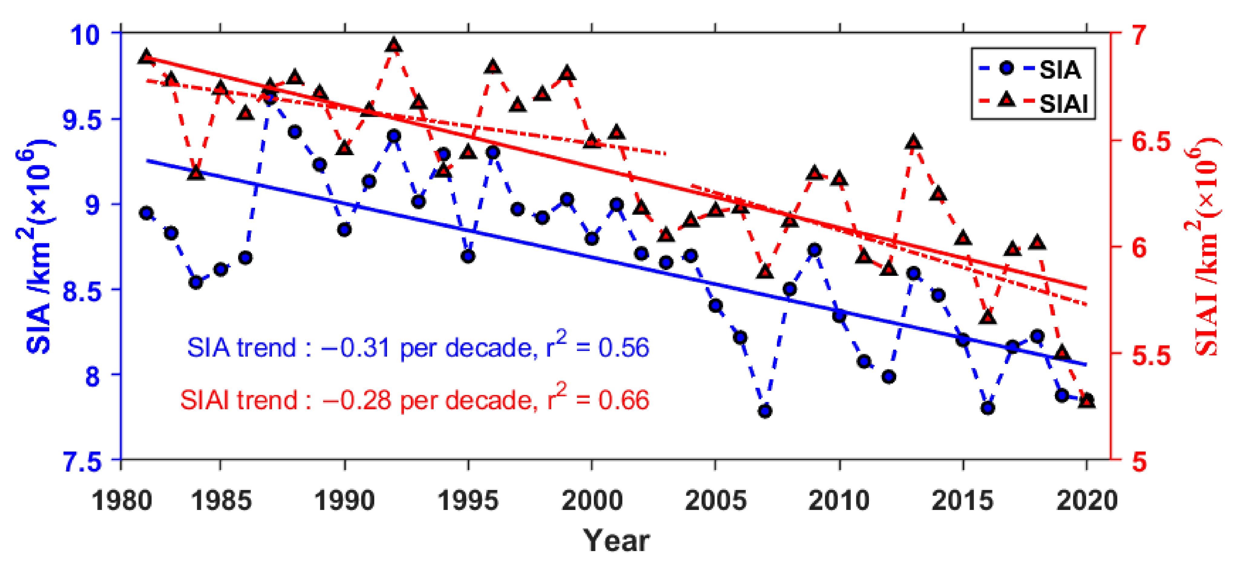
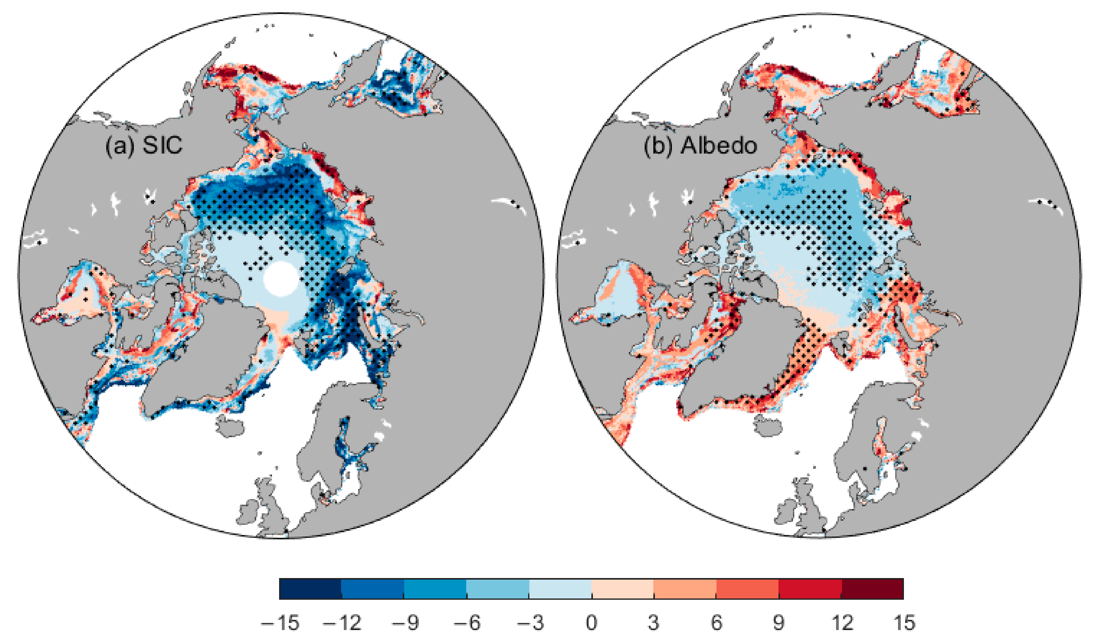
3.1. The Change in Arctic Sea Ice Albedo

The unit grid sea ice area is equal to the product of the SIC and grid area, and sea ice area (SIA) is the total of all grids, with each grid having a 625 km2 area. Similarly, the sea ice albedo index (SIAI) is calculated by multiplying the unit grid albedo by the grid area, then summing the product over all grids. Here, we have calculated the annual average SIA and SIAI from March to September based on the satellite-monitored SIC and albedo, and the results are shown in Figure 1. During March to September, the average SIA and SIAI in the Arctic decreased by about 1.2 million km2 and 1.1 million km2 from 1982 to 2020, respectively. The correlation coefficient of 0.87 for the two metrics is larger than that of 0.78 for Peng et al. [27] (correlation between albedo and extent of Arctic Sea ice from 1982 to 2015). This implies that the decrease in albedo is mainly associated with the reduction in SIA [63]. According to Hegyi and Taylor [64], the efficiency of radiative cooling in the Arctic has declined since 2000. It is clear that the decline trend of SIAI accelerated after 2000, and a Mann-Kendall test analysis shows that this inflection point appeared in 2003. This generally downward trend was interrupted by a relatively cool and cloudy summer in 2013 [65].
Then, we compared the difference before and after the albedo turning point using sea ice albedo from APP-x and SIC from Nimbus-7 SMMR and DMSP SSM/I-SSMIS. The spatial distribution of the average difference in SIC and albedo in the periods 2003–2020 and 1982–2002 is shown in Figure 2. Each pixel value in the figure was obtained by averaging the values from March to September. Although there is a general tendency toward decline but a slight rise in the ice-marginal zone, the disparities in SIC and albedo distribution are largely constant. Over the Beaufort and Chukchi Seas, the Eur-Asian Sea area, and Baffin Bay, the SIC falls most noticeably while increasing over the Bering Sea. The difference between albedo variation and SIC variation is mainly in the marginal sea areas, especially in the Greenland Sea, Barents Sea, Baffin Bay, and Sea of Okhotsk (Figure 2b).

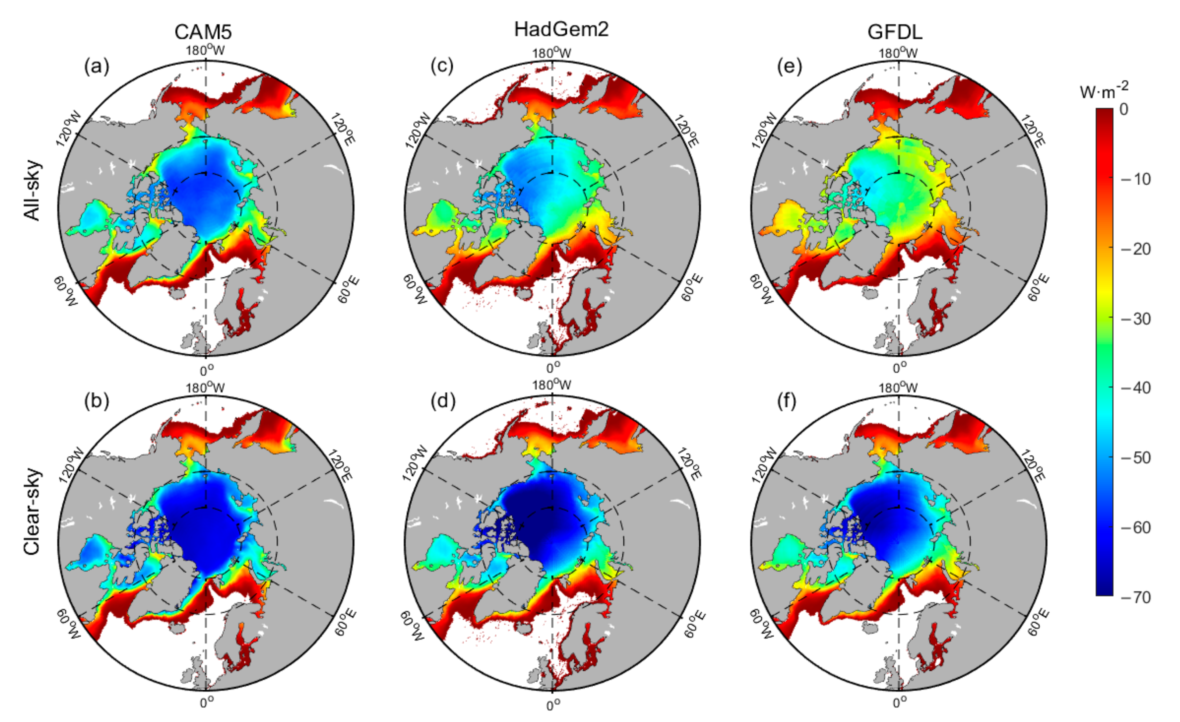
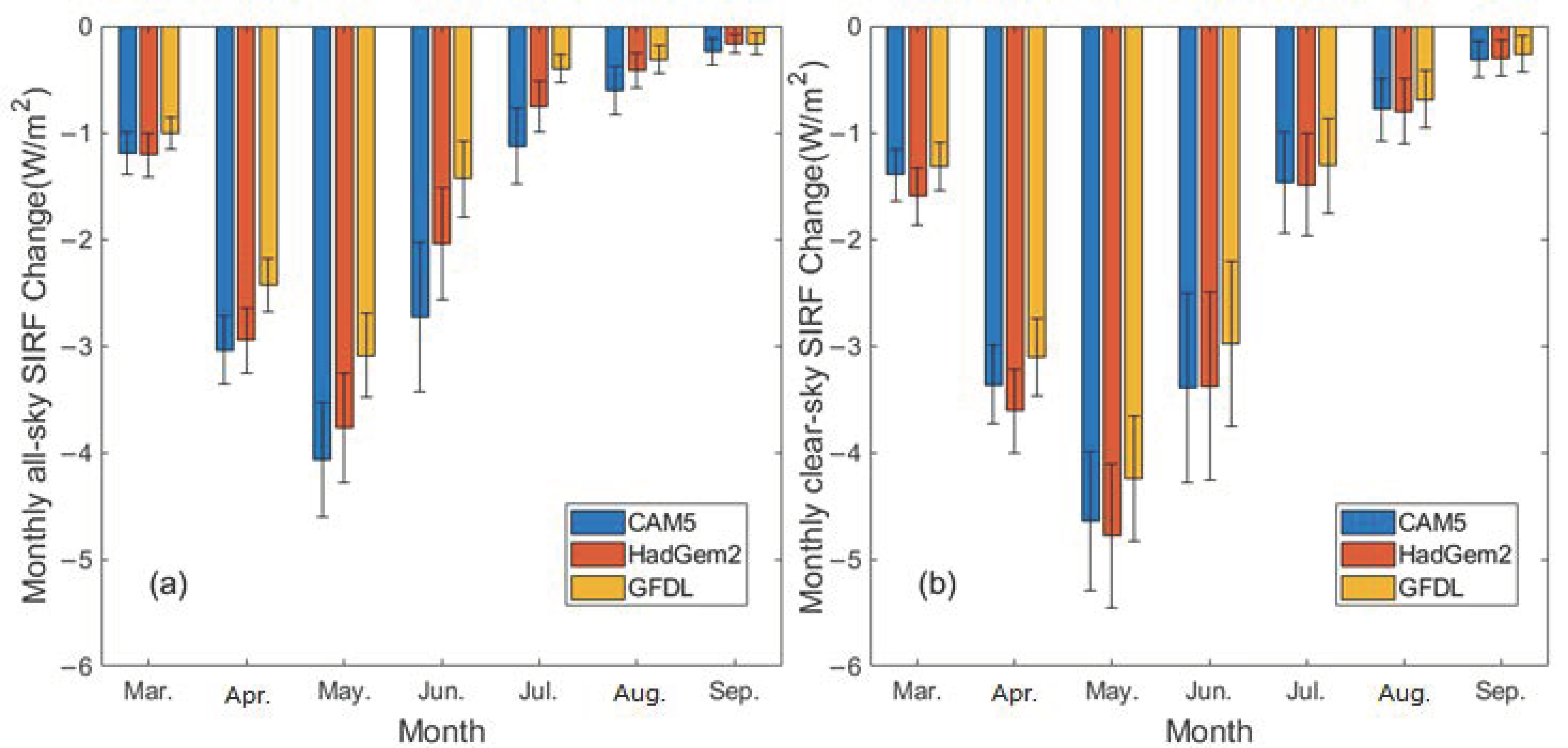
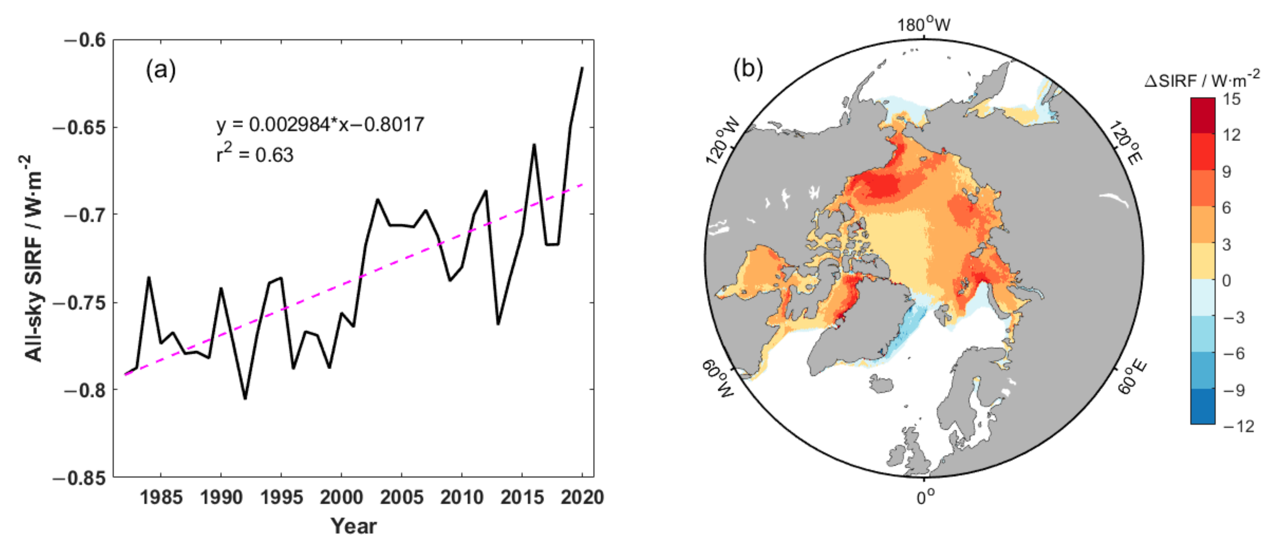
3.2. Arctic SIRF and Seasonal Variation

Based on the three sea ice albedo products and three radiative kernels, we calculated the Arctic clear-sky and all-sky SIRFs, and the average results for 1982–2020 are presented in Table 2. The mean all-sky SIRF with APP-x is −0.93 ± 0.13 W · m 2 , which is close to that of ERA5, −0.95 ± 0.10 W · m 2 , and smaller than that of MERRA2, −1.04 ± 0.11 W · m 2 . The difference between the mean SIRF calculated with different radiative kernels was larger, with a difference of 0.39 W · m 2 between CAM5 and GFDLs all-sky mean SIRF. Only the all-sky SIRF calculated by GFDL was between 0.65 W · m 2 [29] and 0.85 W · m 2 [31], and the other estimates were larger. The results of the clear-sky SIRF showed a consistent change. The main reasons for the differences between radiative kernels are the radiative transfer parameterization and the underlying climatological settings between models, such as the climatic distribution of clouds [46]. We noted that the clear-sky SIRF of CAM5 and HadGem2 are slightly larger than the all-sky SIRF, while the clear-sky SIRF of GFDL is about twice as large as the all-sky SIRF, which is consistent with the results obtained by Cao et al. [31] and Flanner et al. [29]. This difference reflects the attenuating effect of clouds on the cooling effect of sea ice.
We generated average SIRF distribution maps for the entire Arctic Sea ice region over the past 39 years to compare the differences between the three radiating kernels and the differences between all-sky and clear-sky (Figure 3). The highest annual mean SIRF was −70 W · m 2 in the center region of the Arctic to the surrounding areas, which may be related to the late onset of melting in this area. As is shown in Figure 3a, the SIRF in Hudson Bay can also reach more than −40 W · m 2 , which is not negligible. The all-sky SIRF calculated from various kernels has a higher difference than the clear-sky SIRF. The results of the GFDL estimated SIRF are comparable to those determined by Cao et al. [31]. Overall, GFDLs estimates of SIRF magnitudes are less than those made by CAM5 and HadGem2.
The seasonal variation of the mean SIRF within the study region is shown in Figure 4. Both the all-sky SIRF and clear-sky SIRF have a consistent pattern of change, culminating around May. According to the results of Light et al. [66], which compared the average total albedo for MOSAiC and SHEBA campaign observations, the albedo of the ice surface is above 0.8 in April–May and decreases to approximately 0.4 from June until early August. As a result, from March to May, the SIRF steadily increases with the solar altitude angle. The sea ice begins to melt in June, which causing a decrease in surface albedo and sea ice extent and a quick decline in the SIRF to less than −1 W · m 2 in August and September. Huang et al. [67] found that the accumulation of radiative energy in the early months could well explain the sea ice extent change in September (R2 = 0.81), and there was a strong correlation with the radiative anomaly in June. The maximum fluctuation of SIRF was observed in May and June (Figure 4), which influenced the change in air temperature through radiative feedback. Therefore, the CRS of Arctic sea ice through albedo mainly occurs from April to June.

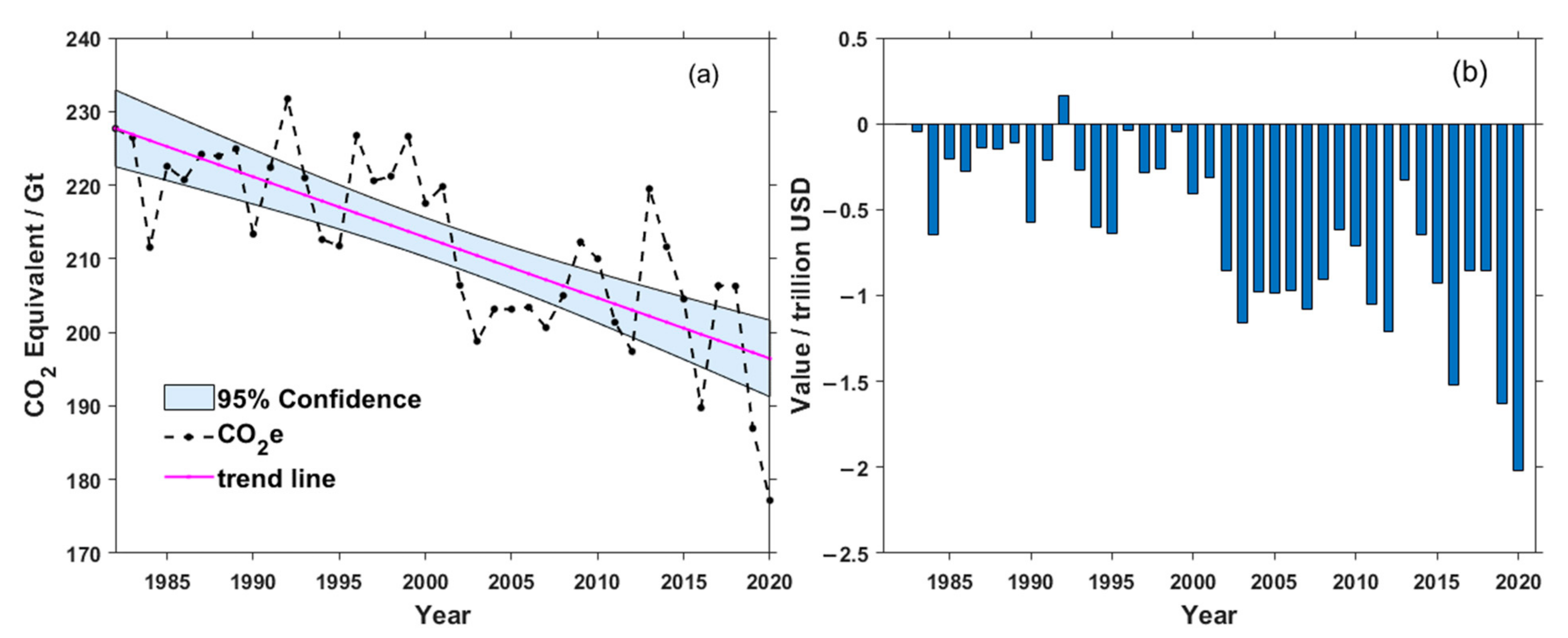
3.3. Past SIRF Changes and Economic Impacts

In this section, we analyze the trends and the economic damage for 1982–2020 using the all-sky SIRF estimated by APP-x and GFDL. The SIRF increased significantly during the satellite monitoring period, with a total SIRF increase of 0.12 W · m 2 and an annual average increase of 0.002984 W · m 2 (Figure 5a). The SIRF grew from 2001 to 2003 by 0.07 W · m 2 , and starting in this period, it began to climb more quickly, which is consistent with the shift in the SIAI. A hot wave in the Siberian region caused an early melting of the Arctic Sea ice and an increase in average temperature of 8–10 °C, according to the Arctic Report Card 2020: Sea Ice [68]. As a result, the minimum sea ice extent was the second lowest on record. Additionally, due to this extreme weather event, the SIRF reached a minimum of −0.62 W · m 2 . Figure 5b shows the spatial distribution of SIRF changes from 1982 to 2020. A positive (negative) ∆SIRF represents an increase (decrease) in radiative forcing. Seong et al. [33] indicated that the regions with the largest changes in SIRF were the Kara Sea and Barents Sea, and we discovered that the Beaufort Sea and eastern side of Baffin Bay also increased significantly. However, there are a few areas where the SIRF shows an increasing trend, such as the Barents Sea and the Greenland Sea. Selyuzhenok et al. [69] found that the increased volume flux of sea ice through the Fram Strait occurred parallel with a decrease in sea ice in the Greenland Sea. The input of high-albedo sea ice from high latitudes compensates for the melting and reduced albedo, which is responsible for the reduced SIRF in this region.
The average Arctic all-sky SIRF for 1982–2020 was −0.75 ± 0.10 W · m 2 , which is 212.1 ± 28.8 Gt after conversion to CO2 equivalent emissions using the DICE model. The SIRF has been increasing by 0.12 W · m 2 over the last 39 years, which is equivalent to an additional 34.5 Gt of CO2 in the atmosphere. The shaded part of Figure 6a shows the range in which the fit test passes the 95% threshold when the regression coefficient is 0.64. Figure 6b shows the loss of economic value resulting from the annual SIRF change relative to 1982 with a SCC of 40 USD/ton. With the exception of 1992, all years present negative values, accumulating to −24.4 trillion USD. When the SCC was between 40 and 80 USD/ton in 2020, the economic loss was between 24.4 and 48.8 trillion USD.

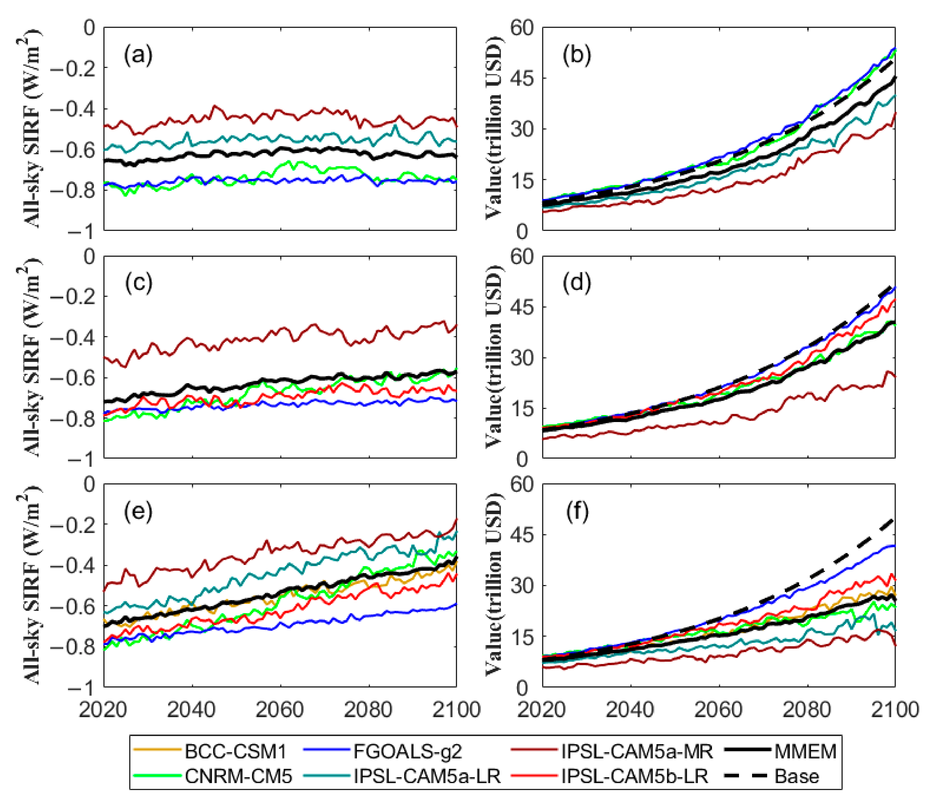
3.4. Projected Future Arctic SIRF Changes and Economic Impacts

Here, the climatological sea ice albedo for three emission scenarios (including RCP2.6, RCP4.5, and RCP8.5) are counted by making differential comparisons from 70°N (Table 3). The multi-model ensemble mean (MMEM) refers to the average of the six CMIP5 models used in this study. Note that most CMIP5 models overestimate the sea ice albedo in the Arctic, and the RCP2.6 ensemble has the smallest mean value, MAE, and RMSE, at 0.06, 0.09, and 0.13, respectively. Although the MMEM and APP-x are nearly similar, there are still substantial variations between these models. For example, IPSL-CAM5a-LR has the smallest mean of 0.03, while CNRM-CM5 has means of 0.15 and 0.16 for the RCP2.6 and RCP8.5 scenarios, respectively. Overall, there is a small amount of uncertainty when estimating future Arctic SIRF changes and economic loss storage using CMIP5 MMEM sea ice albedo data.
We estimated the all-sky SIRF for 2020–2100 using the GFDL kernel with the CMIP5 model’s sea ice albedo. As is shown in Figure 7a,c,e, the future SIRF is projected to increase under all three scenarios, although it only begins to increase slightly by the end of the twenty-first century under the RCP2.6 scenario. The SIRF in RCP4.5 increased by 0.14 W · m 2 , and the SIRF of RCP8.5 increased twice as much, by 0.31 W · m 2 . Among all models, the SIRF of FGOALS-g2 is the smallest and the largest is IPSL-CAM5a-MR.
The projected value trends pertinent to various climate change scenarios after 2020 are described in Figure 7b,d,f. The loss of these economic benefits would come entirely from the increase in SIRF associated with “business as usual (black dashed line)”. Based on a 2020 SCC of 40 USD/ton and a discount rate of 2.3%, a SCC of 80 USD/ton is twice its value. When climate change is limited to the RCP2.6 scenario, the cumulative value loss of the MMEM in the Arctic would be 243.7–487.4 trillion USD; the loss under the RCP4.5 scenario would be 325.7–651.4 trillion USD, and the loss under the RCP8.5 scenario would be 565.3–1130.6 trillion USD. After 2040, the differences between the three emissions scenarios become apparent.
These results illustrate a large difference between the model and emission scenarios for future SIRF and CRS value losses. The difference in sea ice albedo between models reflects the uncertainty of sea ice prediction. More efforts to curb carbon emissions and adopt sustainable approaches can reduce the loss of more CRS economic value of the Arctic Sea ice albedo.

4. Discussion

4.1. Comparison with Previous Studies

In this study, we have evaluated the SIRF of sea ice albedo change over the past 39 years and projected it from 2020 to 2100 at the global scale. We used albedo data from March to September to calculate the SIRF for the whole Arctic since the SIRF from October to February is only approximately 4% of the year [31]. Around 2003, the trend of decreasing mean sea ice albedo from March to September started to accelerate, and the reasons for this change require more investigation outside the scope of this work. Arctic sea ice has declined nearly twice as rapidly since 2000 (e.g., [70]). It has been demonstrated that increasing cloud cover could have contributed significantly to the recent and historical sea ice changes [71,72]. The minimum average SIA happened in 2007, whereas the minimum SIAI occurred in 2020 (Figure 1), indicating that not only the sea ice cover but also the snow accumulation on ice and early melting may have significant effects on the albedo [12]. Although there is a general tendency for albedo to decrease, it is interesting to notice that the opposite variation occurs in marginal sea. The increasing albedo in the Greenland Sea is attributable to the increased sea ice output, while the reason for the increases in other sea regions remains uncertain.
Previous studies have demonstrated that the SIRF in the Arctic has increased rapidly during the satellite era [29,31,32,33]. Here, we obtained similar results based on the radiative kernel method, which indicated a more pronounced increase after 2003. Specifically, the 2020 SIRF is the highest in the observational record. These results may reflect the transition to a new dynamic state over the last two decades with the triggering of positive feedback in the Arctic climate system [73]. The role of snowline retreat in albedo decrease is comparable to that of sea ice shrinking in the Northern Hemisphere [74], with an annual mean radiative forcing of 0.56–0.73 W · m 2 [75,76]. In addition, increasing CO2 and methane emissions from thawing permafrost contribute to global warming. Pistone et al. [37] and Euskirchen et al. [41] estimated global radiative forcing of 0.71 W · m 2 and 0.8–1.6 W · m 2 for sea ice under complete loss and CMIP3 sea ice reduction, respectively. Our findings show that by 2100, the RCP8.5 scenario will have resulted in a rise of just 0.31 W · m 2 in the SIRF, which is far less than the previous results. This discrepancy may be due to different postulated conditions. According to the seasonal evolution of sea ice, the possibility of April–June each year being completely ice-free, which is the time of maximum SIRF, is low and may not occur.
It is difficult to assess the economic impacts of climate change. As the IPCC AR6 demonstrates, while our understanding of climate change effects is rapidly improving, there are still no good models readily available that can be easily applied to our economic analysis [77]. Yumashev et al. [43] explored the nonlinear changes in Arctic feedbacks under different temperature target scenarios of the Paris Agreement and their subsequent impacts on the global climate and economy through the integrated assessment model PAGE-ICE. The assessment by Euskirchen et al. [41] was divided into four scenarios based on the SCC and discount rates of different institutions. Here, the economic costs of future SIRF under three pathways (RCP2.6, RCP4.5, and RCP8.5) are estimated based on the SCC of 40–80 USD/ton and a stable discount rate, which are required to achieve the Paris Agreement targets. By 2100, the cumulative cost under the RCP8.5 scenario is 565.3–1130.6 trillion USD. This is a lot more than that calculated by Euskirchen et al. [41], and the main reason for this difference is the choice of SCC, discount rate, and SIRF. HERE

4.2. Uncertainties

The sea ice albedo products and radiative kernels are the sources of the uncertainty in the SIRF estimates. SIRFs estimations show that ERA5s sea ice albedo is closer to APP-x than to MERRA2s. Moreover, the difference in sea ice albedo between model outputs in CMIP5 is very large, e.g., that of FGOALS-g2 is almost twice as large as that of IPSL-CAM5a-MR. Since model simulations still underestimate the sensitivity of Arctic Sea ice to climate change [78], we may also underestimate the long term change in SIRF. The difference between the radiative kernels is mainly determined by the bias of the climate models. Kramer et al. [79] found that the size and structure of radiative kernels derived from observational data are consistent with those of the GFDL kernel. Consequently, the GFDL kernel is used in our estimation of past and future SIRF.
The economic uncertainties are far bigger than the potential future feedback effects, which are mainly related to the SCC [41]. The SCC is used to help policymakers determine whether the costs and benefits of a proposed policy to curb climate change are justified. A high SCC usually means that the benefits of a particular climate policy are justified in terms of CO2 reductions; a low SCC makes it appear that the costs of a policy outweigh the benefits it will ultimately bring. The main driver of the differences in SCC across time is the choice of discount rate. If the discount rate is large, future consequences are given significantly less weight than immediate ones, whereas if it’s low, they’re given about the same weight. In this study, we assumed only the boundary benefit under the Paris temperature target to estimate the economic cost arising from future SIRF changes.

5. Conclusions

This study assessed the variation of SIRF over the Arctic region from 1982 to 2100 using a radiative kernel method, and estimated the cost of the lost sea ice regulating service. The APP-x dataset’s historical analysis aids in our knowledge of Arctic Sea ice change, and the CMIP5 dataset’s projection of the associated economic cost assessment may inform future policymaking.
The results showed an average SIRF of −0.75 ± 0.10 W · m 2 for the Arctic from 1982 to 2020, with a total increase of 0.12 W · m 2 , equivalent to 34.5 Gt of CO2 emitted into the atmosphere and a cumulative loss of 24.4–48.8 trillion USD. With the decrease of SIA and SIC, SIRF has been increasing rapidly since 2003. Spatially, the SIRF is increasing in almost the entire Arctic Ocean, especially in the Beaufort Sea, Baffin Bay, and the Barents Sea. The only marine region showing a major decline is the Greenland Sea, and this is due to the constant flow of sea ice from higher latitudes via the Flam Strait. From 2020 to 2100, the maximum increase in SIRF for RCP8.5 is predicted to be 0.31 W · m 2 , with an average annual economic cost of 6.7–13.3 trillion USD. It is found that the economic cost to society of future SIRF changes could be achieved by adopting additional methods of reducing CO2 emissions and sustainability.
Over the past two decades, the accelerated melting of Arctic sea ice and the increase of snow cover extent in the northern Hemisphere [75] are pointing to a new state of the Arctic climate system. However, the specific reasons for this shift and the connection between sea ice and snow extent changes remain unclear. To provide a more complete picture of the effects and costs of cryosphere changes, it is also necessary to evaluate the melting of snow and permafrost using the methodology used in this research. Additionally, it is essential to combine climate science, economics, and policy studies in order to give a full evaluation of climate change’s effects.

Author Contributions

Conceptualization, H.H. and B.S.; methodology, H.H. and S.L.; software, H.H. and S.L.; validation, H.H.; writing—original draft preparation, H.H. and W.Z.; writing—review and editing, B.S. and S.L. All authors have read and agreed to the published version of the manuscript.

Funding

This study is supported by the International Cooperation Team on Key Processes and Impacts of the Arctic Cryosphere (BNU 2022-GJTD-01) and the Early-Career Fellowship (2022 Annual Program to Bo Su) of Future Earth Global Secretariat Hub China.

Data Availability Statement

The Arctic ice albedo products from the Extended Advanced Very High-Resolution Radiometer Polar Pathfinder (APP-x) analyzed in this study are freely available at https://www.ncei.noaa.gov/products (accessed on 19 November 2022). The albedo of MERRA-2 can be request from https://disc.gsfc.nasa.gov/datasets (accessed on 19 November 2022). The albedo of ERA5 can be requested from ECMWF (https://cds.climate.copernicus.eu, accessed on 19 November 2022). The albedo of CMIP5 can be download from https://data.ceda.ac.uk/badc/cmip5/data/cmip5/ (accessed on 19 November 2022). The CAM5 is available at https://climatedataguide.ucar.edu/climate-data/radiative-kernels-climate-models (accessed on 19 November 2022). The HadGEM2 is available at http://homepages.see.leeds.ac.uk/~mencsm/kernels.htm (accessed on 19 November 2022). The GFDL is available at https://climate.earth.miami.edu/data/radiative-kernels/index.html (accessed on 19 November 2022). The sea ice concentration can be requested from NSIDC (https://nsidc.org/data, accessed on 19 November 2022).

Acknowledgments

We are grateful to editors and three anonymous reviewers for their insightful and generous comments.

Conflicts of Interest

The authors declare no conflict of interest.

References

  1. Serreze, M.C.; Barry, R.G. Processes and impacts of Arctic amplification: A research synthesis. Glob. Planet. Change 2011, 77, 85–96. [Google Scholar]
  2. Rantanen, M.; Karpechko, A.Y.; Lipponen, A.; Nordling, K.; Hyvärinen, O.; Ruosteenoja, K.; Vihma, T.; Laaksonen, A. The Arctic has warmed nearly four times faster than the globe since 1979. Commun. Earth Environ. 2022, 3, 168. [Google Scholar] [CrossRef]
  3. Dai, A.; Luo, D.; Song, M.; Liu, J. Arctic amplification is caused by sea-ice loss under increasing CO2. Nat. Commun. 2019, 10, 121. [Google Scholar] [CrossRef]
  4. Screen, J.A.; Simmonds, I. The central role of diminishing sea ice in recent Arctic temperature amplification. Nature 2010, 464, 1334–1337. [Google Scholar] [CrossRef]
  5. Comiso, J.C. Large decadal decline of the Arctic multiyear ice cover. J. Clim. 2012, 25, 1176–1193. [Google Scholar] [CrossRef]
  6. Peng, G.; Meier, W.N. Temporal and regional variability of Arctic sea-ice coverage from satellite data. Ann. Glaciol. 2018, 59, 191–200. [Google Scholar] [CrossRef]
  7. Kwok, R. Arctic sea ice thickness, volume, and multiyear ice coverage: Losses and coupled variability (1958–2018). Environ. Res. Lett. 2018, 13, 105005. [Google Scholar] [CrossRef]
  8. Kwok, R.; Cunningham, G.F. Variability of Arctic sea ice thickness and volume from CryoSat-2. Philos. Trans. R. Soc. A Math. Phys. Eng. Sci. 2015, 373, 20140157. [Google Scholar] [CrossRef]
  9. Markus, T.; Stroeve, J.C.; Miller, J. Recent changes in Arctic sea ice melt onset, freezeup, and melt season length. J. Geophys. Res. 2009, 114, C12024. [Google Scholar]
  10. Stroeve, J.C.; Markus, T.; Boisvert, L.N.; Miller, J.A.; Barrett, A.P. Changes in Arctic Melt Season and Implications for Sea Ice Loss. Geophys. Res. Lett. 2014, 41, 1216–1225. [Google Scholar] [CrossRef]
  11. Smith, A.; Jahn, A.; Burgard, C.; Notz, D. Improving model-satellite comparisons of sea ice melt onset with a satellite simulator. Cryosphere Discuss. 2021, 16, 3235–3248. [Google Scholar] [CrossRef]
  12. Perovich, D.K.; Polashenski, C. Albedo evolution of seasonal Arctic sea ice. Geophys. Res. Lett. 2012, 39, L08501. [Google Scholar] [CrossRef]
  13. Riihelä, A.; Manninen, T.; Laine, V. Observed changes in the albedo of the Arctic sea-ice zone for the period 1982–2009. Nat. Clim. Chang. 2013, 3, 895–898. [Google Scholar] [CrossRef]
  14. Xiao, C.D.; Wang, S.J.; Qin, D.H. A preliminary study of cryosphere service function and value evaluation. Adv. Clim. Chang. Res. 2015, 6, 181–187. [Google Scholar] [CrossRef]
  15. Su, B.; Xiao, C.; Chen, D.; Qin, D.; Ding, Y. Cryosphere services and human well-being. Sustainability 2019, 11, 4365. [Google Scholar] [CrossRef]
  16. Xiao, C.; Su, B.; Wang, X.; Qin, D. Cascading risks to the deterioration in cryospheric functions and services. Kexue Tongbao Chin. Sci. Bull. 2019, 64, 1975–1984. [Google Scholar] [CrossRef]
  17. Gacheno, D.; Amare, G. Review of Impact of Climate Change on Ecosystem Services—A Review. Int. J. Food Sci. Agric. 2021, 5, 363–369. [Google Scholar] [CrossRef]
  18. Burke, M.; Hsiang, S.M.; Miguel, E. Global non-linear effect of temperature on economic production. Nature 2015, 527, 235–239. [Google Scholar] [CrossRef]
  19. Whiteman, G.; Hope, C.; Wadhams, P. Vast costs of Arctic change—Methane released by melting permafrost will have global impacts. Nature 2013, 499, 401–403. [Google Scholar] [CrossRef]
  20. Andry, O.; Bintanja, R.; Hazeleger, W. Time-dependent variations in the Arctic’s surface albedo feedback and the link to seasonality in sea ice. J. Clim. 2017, 30, 393–410. [Google Scholar] [CrossRef]
  21. Thackeray, C.W.; Hall, A. An emergent constraint on future Arctic sea-ice albedo feedback. Nat. Clim. Chang. 2019, 9, 972–978. [Google Scholar] [CrossRef]
  22. Petrich, C.; Eicken, H.; Polashenski, C.M.; Sturm, M.; Harbeck, J.P.; Perovich, D.K.; Finnegan, D.C. Snow dunes: A controlling factor of melt pond distribution on Arctic sea ice. J. Geophys. Res. Ocean. 2012, 117, C09029. [Google Scholar] [CrossRef]
  23. Kashiwase, H.; Ohshima, K.I.; Nihashi, S.; Eicken, H. Evidence for ice-ocean albedo feedback in the Arctic Ocean shifting to a seasonal ice zone. Sci. Rep. 2017, 7, 8170. [Google Scholar] [CrossRef]
  24. Pinker, R.T.; Niu, X.M.; Ma, Y. Solar heating of the Arctic Ocean in the context of ice-albedo feedback. J. Geophys. Res. Ocean. 2014, 119, 8395–8409. [Google Scholar] [CrossRef]
  25. Letterly, A.; Key, J.; Liu, Y. Arctic climate: Changes in sea ice extent outweigh changes in snow cover. Cryosphere 2018, 12, 3373–3382. [Google Scholar] [CrossRef]
  26. Graversen, R.G.; Wang, M. Polar amplification in a coupled climate model with locked albedo. Clim. Dyn. 2009, 33, 629–643. [Google Scholar] [CrossRef]
  27. Peng, H.T.; Ke, C.Q.; Shen, X.; Li, M.; Shao, Z. De Summer albedo variations in the Arctic Sea ice region from 1982 to 2015. Int. J. Climatol. 2020, 40, 3008–3020. [Google Scholar] [CrossRef]
  28. Zhang, R.; Wang, H.; Fu, Q.; Rasch, P.J.; Wang, X. Unraveling driving forces explaining significant reduction in satellite-inferred Arctic surface albedo since the 1980s. Proc. Natl. Acad. Sci. USA 2019, 116, 23947–23953. [Google Scholar] [CrossRef]
  29. Flanner, M.G.; Shell, K.M.; Barlage, M.; Perovich, D.K.; Tschudi, M.A. Radiative forcing and albedo feedback from the Northern Hemisphere cryosphere between 1979 and 2008. Nat. Geosci. 2011, 4, 151–155. [Google Scholar] [CrossRef]
  30. Pistone, K.; Eisenman, I.; Ramanathan, V. Observational determination of albedo decrease caused by vanishing Arctic sea ice. Proc. Natl. Acad. Sci. USA 2014, 111, 3322–3326. [Google Scholar] [CrossRef]
  31. Cao, Y.; Liang, S.; Chen, X.; He, T. Assessment of sea ice albedo radiative forcing and feedback over the Northern Hemisphere from 1982 to 2009 using satellite and reanalysis data. J. Clim. 2015, 28, 1248–1259. [Google Scholar] [CrossRef]
  32. Riihelä, A.; Bright, R.M.; Anttila, K. Recent strengthening of snow and ice albedo feedback driven by Antarctic sea-ice loss. Nat. Geosci. 2021, 14, 832–836. [Google Scholar] [CrossRef]
  33. Seong, N.-H.; Kim, H.-C.; Choi, S.; Jin, D.; Jung, D.; Sim, S.; Woo, J.; Kim, N.; Seo, M.; Lee, K.-S.; et al. Evaluation of Sea Ice Radiative Forcing according to Surface Albedo and Skin Temperature over the Arctic from 1982–2015. Remote Sens. 2022, 14, 2512. [Google Scholar] [CrossRef]
  34. Holland, M.M.; Serreze, M.C.; Stroeve, J. The sea ice mass budget of the Arctic and its future change as simulated by coupled climate models. Clim. Dyn. 2010, 34, 185–200. [Google Scholar] [CrossRef]
  35. Overland, J.E.; Wang, M. When will the summer Arctic be nearly sea ice free? Geophys. Res. Lett. 2020, 40, 2097–2101. [Google Scholar] [CrossRef]
  36. Niederdrenk, A.L.; Notz, D. Arctic Sea Ice in a 1.5 °C Warmer World. Geophys. Res. Lett. 2018, 45, 1963–1971. [Google Scholar] [CrossRef]
  37. Pistone, K.; Eisenman, I.; Ramanathan, V. Radiative Heating of an Ice-Free Arctic Ocean. Geophys. Res. Lett. 2019, 46, 7474–7480. [Google Scholar] [CrossRef]
  38. Hudson, S.R. Estimating the global radiative impact of the sea ice-albedo feedback in the Arctic. J. Geophys. Res. Atmos. 2011, 116, D16102. [Google Scholar] [CrossRef]
  39. Notz, D.; Stroeve, J. The Trajectory Towards a Seasonally Ice-Free Arctic Ocean. Curr. Clim. Chang. Rep. 2018, 4, 407–416. [Google Scholar] [CrossRef]
  40. Crawford, A.; Stroeve, J.; Smith, A.; Jahn, A. Arctic open-water periods are projected to lengthen dramatically by 2100. Commun. Earth Environ. 2021, 2, 109. [Google Scholar] [CrossRef]
  41. Euskirchen, E.S.; Goodstein, E.S.; Huntington, H.P. An estimated cost of lost climate regulation services caused by thawing of the Arctic cryosphere. Ecol. Appl. 2013, 23, 1869–1880. [Google Scholar] [CrossRef]
  42. Badina, S.; Pankratov, A. Assessment of the Impacts of Climate Change on the Russian Arctic Economy (including the Energy Industry). Energies 2022, 15, 2849. [Google Scholar] [CrossRef]
  43. Yumashev, D.; Hope, C.; Schaefer, K.; Riemann-Campe, K.; Iglesias-Suarez, F.; Jafarov, E.; Burke, E.J.; Young, P.J.; Elshorbany, Y.; Whiteman, G. Climate policy implications of nonlinear decline of Arctic land permafrost and other cryosphere elements. Nat. Commun. 2019, 10, 1900. [Google Scholar] [CrossRef]
  44. Nordhaus, W.D.; Boyer, J. Warming the World: Economic Models of Global Warming; The MIT Press: Cambridge, MA, USA, 2000; Volume 7. [Google Scholar]
  45. Nordhaus, W. Economics of the disintegration of the Greenland ice sheet. Proc. Natl. Acad. Sci. USA 2019, 116, 12261–12269. [Google Scholar] [CrossRef]
  46. Soden, B.J.; Held, I.M.; Colman, R.C.; Shell, K.M.; Kiehl, J.T.; Shields, C.A. Quantifying climate feedbacks using radiative kernels. J. Clim. 2008, 21, 3504–3520. [Google Scholar] [CrossRef]
  47. Seitz, R. Bright water: Hydrosols, water conservation and climate change. Clim. Chang. 2010, 105, 365–381. [Google Scholar] [CrossRef]
  48. Maslanik, J.A.; Key, J.; Fowler, C.W.; Nguyen, T.; Wang, X. Spatial and Temporal Variability of Satellite-derived Cloud and Surface Characteristics During FIRE-ACE. J. Geophys. Res. Atmos. 2001, 106, 233–249. [Google Scholar]
  49. Key, J.; Wang, X.; Liu, Y.; Dworak, R.; Letterly, A. The AVHRR polar Pathfinder climate data records. Remote Sens. 2016, 8, 167. [Google Scholar] [CrossRef]
  50. Van Vuuren, D.P.; Edmonds, J.; Kainuma, M.; Riahi, K.; Thomson, A.; Hibbard, K.; Hurtt, G.C.; Kram, T.; Krey, V.; Lamarque, J.F.; et al. The representative concentration pathways: An overview. Clim. Chang. 2011, 109, 5–31. [Google Scholar] [CrossRef]
  51. Moss, R.H.; Edmonds, J.A.; Hibbard, K.A.; Manning, M.R.; Rose, S.K.; Van Vuuren, D.P.; Carter, T.R.; Emori, S.; Kainuma, M.; Kram, T.; et al. The next generation of scenarios for climate change research and assessment. Nature 2010, 463, 747–756. [Google Scholar] [CrossRef]
  52. Cavalieri, D.; Parkinson, C.; Gloersen, P.; Zwally, H. Sea Ice Concentrations from Nimbus-7 SMMR and DMSP SSM/I-SSMIS Passive Microwave Data, Version 1; NASA National Snow and Ice Data Center Distributed Active Archive Center: Boulder, CO, USA, 1996; p. 29. [Google Scholar] [CrossRef]
  53. Brodzik, M.J.; Billingsley, B.; Haran, T.; Raup, B.; Savoie, M.H. EASE-Grid 2.0: Incremental but significant improvements for earth-gridded data sets. ISPRS Int. J. Geo-Inf. 2012, 1, 32–45. [Google Scholar] [CrossRef]
  54. Gelaro, R.; McCarty, W.; Suárez, M.J.; Todling, R.; Molod, A.; Takacs, L.; Randles, C.A.; Darmenov, A.; Bosilovich, M.G.; Reichle, R.; et al. The modern-era retrospective analysis for research and applications, version 2 (MERRA-2). J. Clim. 2017, 30, 5419–5454. [Google Scholar] [CrossRef]
  55. Hersbach, H.; Bell, B.; Berrisford, P.; Hirahara, S.; Horányi, A.; Muñoz-Sabater, J.; Nicolas, J.; Peubey, C.; Radu, R.; Schepers, D.; et al. The ERA5 global reanalysis. Q. J. R. Meteorol. Soc. 2020, 146, 1999–2049. [Google Scholar] [CrossRef]
  56. Pendergrass, A.G.; Conley, A.; Vitt, F.M. Surface and top-of-Atmosphere radiative feedback kernels for cesm-cam5. Earth Syst. Sci. Data 2018, 10, 317–324. [Google Scholar] [CrossRef]
  57. Smith, C.J.; Kramer, R.J.; Myhre, G.; Forster, P.M.; Soden, B.J.; Andrews, T.; Boucher, O.; Faluvegi, G.; Fläschner, D.; Hodnebrog, M.K.; et al. Understanding Rapid Adjustments to Diverse Forcing Agents. Geophys. Res. Lett. 2018, 45, 12023–12031. [Google Scholar] [CrossRef]
  58. Nordhaus, W.D. Estimates of the Social Cost of Carbon:Concepts and Results from the DICE-2013R Model and Alternative Approaches. SSRN Electron. J. 2014, 1, 273–312. [Google Scholar] [CrossRef]
  59. Nordhaus, W.D. Revisiting the social cost of carbon. Proc. Natl. Acad. Sci. USA 2017, 114, 1518–1523. [Google Scholar] [CrossRef]
  60. World Bank. State and Trends of Carbon Pricing 2021; World Bank: Washington, DC, USA, 2020; ISBN 9781464815867. [Google Scholar]
  61. Moritz, R.E.; Gawel, A. Increasing Climate Ambition: Analysis of an International Carbon Price Floor; World Economic Forum: Geneva, Switzerland; PwC: Geneva, Switzerland, 2021. [Google Scholar]
  62. Stiglitz, J.E.; Stern, N.; Duan, M.; Edenhofer, O.; Giraud, G.; Heal, G.M.; la Rovere, E.L.; Morris, A.; Moyer, E.; Pangestu, M.; et al. Report of the High-Level Commission on Carbon Prices; International Bank for Reconstruction and Development: Washington, DC, USA; International Development Association: Washington, DC, USA, 2017. [Google Scholar]
  63. Comiso, J.C.; Parkinson, C.L.; Gersten, R.; Stock, L. Accelerated decline in the Arctic sea ice cover. Geophys. Res. Lett. 2008, 35, L01703. [Google Scholar] [CrossRef]
  64. Hegyi, B.M.; Taylor, P.C. The Unprecedented 2016–2017 Arctic Sea Ice Growth Season: The Crucial Role of Atmospheric Rivers and Longwave Fluxes. Geophys. Res. Lett. 2018, 45, 5204–5212. [Google Scholar] [CrossRef]
  65. Jeffries, M.O.; Richter-Menge, J.A.; Overland, J.E. Arctic Report Card 2013. Ann. Neurol. 2013, 74, A11–A12. Available online: http://www.arctic.noaa.gov/reportcard (accessed on 14 June 2022).
  66. Light, B.; Smith, M.M.; Perovich, D.K.; Webster, M.A.; Holland, M.M.; Linhardt, F.; Raphael, I.A.; Clemens-Sewall, D.; Macfarlane, A.R.; Anhaus, P.; et al. Arctic sea ice albedo: Spectral composition, spatial heterogeneity, and temporal evolution observed during the MOSAiC drift. Elementa 2022, 10, 000103. [Google Scholar] [CrossRef]
  67. Huang, Y.; Chou, G.; Xie, Y.; Soulard, N. Radiative Control of the Interannual Variability of Arctic Sea Ice. Geophys. Res. Lett. 2019, 46, 9899–9908. [Google Scholar] [CrossRef]
  68. Perovich, D.; Meier, W.; Tschudi, M.; Hendricks, S.; Petty, A.A.; Divine, D.; Farrell, S.; Gerland, S.; Haas, C.; Kaleschke, L.; et al. Arctic Report Card 2020: Sea ice. NOAA Arct. Rep. Card 2020 2021. [Google Scholar] [CrossRef]
  69. Selyuzhenok, V.; Bashmachnikov, I.; Ricker, R.; Vesman, A.; Bobylev, L. Sea ice volume variability and water temperature in the Greenland Sea. Cryosphere 2020, 14, 477–495. [Google Scholar] [CrossRef]
  70. Chen, J.L.; Kang, S.C.; Meng, X.H.; You, Q.L. Assessments of the Arctic amplification and the changes in the Arctic sea surface. Adv. Clim. Chang. Res. 2019, 10, 193–202. [Google Scholar] [CrossRef]
  71. Chernokulsky, A.V.; Esau, I.; Bulygina, O.N.; Davy, R.; Mokhov, I.I.; Outten, S.; Semenov, V.A. Climatology and interannual variability of cloudiness in the Atlantic Arctic from surface observations since the late nineteenth century. J. Clim. 2017, 30, 2103–2120. [Google Scholar] [CrossRef]
  72. Huang, Y.; Dong, X.; Bailey, D.A.; Holland, M.M.; Xi, B.; DuVivier, A.K.; Kay, J.E.; Landrum, L.L.; Deng, Y. Thicker Clouds and Accelerated Arctic Sea Ice Decline: The Atmosphere-Sea Ice Interactions in Spring. Geophys. Res. Lett. 2019, 46, 6980–6989. [Google Scholar] [CrossRef]
  73. Matveeva, T.A.; Semenov, V.A. Regional Features of the Arctic Sea Ice Area Changes in 2000–2019 versus 1979–1999 Periods. Atmosphere 2022, 13, 1434. [Google Scholar] [CrossRef]
  74. Marcianesi, F.; Aulicino, G.; Wadhams, P. Arctic sea ice and snow cover albedo variability and trends during the last three decades. Polar Sci. 2021, 28, 100617. [Google Scholar] [CrossRef]
  75. Chen, X.; Yang, Y.; Yin, C. Contribution of changes in snow cover extent to shortwave radiation perturbations at the top of the atmosphere over the northern hemisphere during 2000–2019. Remote Sens. 2021, 13, 4938. [Google Scholar] [CrossRef]
  76. Liu, S.; Qi, J.; Liang, S.; Wang, X.; Wu, X.; Xiao, C. Cascading costs of snow cover reduction trend in northern hemisphere. Sci. Total Environ. 2022, 806, 150970. [Google Scholar] [CrossRef]
  77. Jarraud, M.; Steiner, A. Summary for Policymakers. Managing the Risks of Extreme Events and Disasters to Advance Climate Change Adaptation: Special Report of the Intergovernmental Panel on Climate Change; Cambridge University Press: Cambridge, UK, 2012; Volume 9781107025, pp. 3–22. [Google Scholar] [CrossRef]
  78. Notz, D.; Community, S. Arctic Sea Ice in CMIP6. Geophys. Res. Lett. 2020, 47, e2019GL086749. [Google Scholar] [CrossRef]
  79. Kramer, R.J.; Matus, A.V.; Soden, B.J.; L’Ecuyer, T.S. Observation-Based Radiative Kernels From CloudSat/CALIPSO. J. Geophys. Res. Atmos. 2019, 124, 5431–5444. [Google Scholar] [CrossRef]
Figure 1. Long-term trends of sea ice area (SIA) and sea ice albedo index (SIAI) during March to September in the Arctic. The correlation coefficient is also shown.
Remotesensing 15 00970 g001
Figure 2. Spatial distribution of the average difference in (a) SIC and (b) albedo in the periods 2003–2020 and 1982–2002. The dots show where the SIC and albedo pass the 95% significance test.
Remotesensing 15 00970 g002
Figure 3. The annual mean spatial distribution of all-sky and clear-sky SIRFs for 1982–2020 is calculated based on APP-x and three radiative kernels. (a) CAM5 all-sky. (b) CAM5 clear-sky. (c) HadGem2 all-sky. (d) HadGem2 clear-sky. (e) GFDL all-sky. and (f) GFDL clear-sky.
Remotesensing 15 00970 g003
Figure 4. Month-scale variation in mean SIRF from March to September of (a) all-sky and (b) clear-sky. The vertical black line is the fluctuation range.
Remotesensing 15 00970 g004
Figure 5. Arctic all-sky SIRF changes from 1982 to 2020. (a) Time series of annual mean SIRF in the Arctic. (b) Spatial distribution of ∆SIRF.
Remotesensing 15 00970 g005
Figure 6. (a) Time series of CO2 equivalent of all-sky SIRF from 1982 to 2020. (b) Economic value losses relative to 1982.
Remotesensing 15 00970 g006
Figure 7. Time series of Arctic SIRF and its economic value during 2020–2100 (a,b) RCP2.6. (c,d) RCP4.5. (e,f) RCP8.5.
Remotesensing 15 00970 g007
Table 2. Arctic sea ice radiative forcing ( W · m 2 ), averaged over 1982–2020 and three kernels’ estimates for three albedo products (APP-x, MERRA2, and ERA5).
All-SkyClear-Sky
CAM5HadGem2GFDLMeanCAM5HadGem2GFDLMean
APP-x−1.09 ± 0.16−0.95 ± 0.13−0.75 ± 0.10−0.93 ± 0.13−1.29 ± 0.20−1.34 ± 0.21−1.16 ± 0.19−1.26 ± 0.20
MERRA2−1.25 ± 0.16−1.07 ± 0.10−0.81 ± 0.07−1.04 ± 0.11−1.51 ± 0.16−1.56 ± 0.17−1.34 ± 0.15−1.47 ± 0.16
ERA5−1.13 ± 0.12−0.97 ± 0.10−0.75 ± 0.07−0.95 ± 0.10−1.36 ± 0.16−1.40 ± 0.17−1.22 ± 0.15−1.33 ± 0.16
Mean−1.16 ± 0.15−1.00 ± 0.11−0.77 ± 0.08 −1.39 ± 0.17−1.43 ± 0.18−1.24 ± 0.16
Table 3. Sea ice albedo difference statistics between CMIP5 and APP-x in the 70°N range from 2006 to 2020.
Model RCP2.6 RCP4.5 RCP8.5
MeanMAERMSEMeanMAERMSEMeanMAERMSE
BCC-CSM1nannannannannannan−0.050.150.17
CNRM-CM50.150.150.20−0.050.150.170.160.170.21
FGOALS-g20.130.150.220.160.160.210.120.150.21
IPSL-CAM5a-LR0.030.080.11nannannan0.030.090.12
IPSL-CAM5a-MR−0.070.090.110.130.150.21−0.060.080.10
IPSL-CAM5b-LRnannannan−0.050.070.090.130.150.22
MMEM0.060.090.130.090.110.160.090.110.15
Disclaimer/Publisher’s Note: The statements, opinions and data contained in all publications are solely those of the individual author(s) and contributor(s) and not of MDPI and/or the editor(s). MDPI and/or the editor(s) disclaim responsibility for any injury to people or property resulting from any ideas, methods, instructions or products referred to in the content.

