Study on Influencing Factors of the Information Content of Satellite Remote-Sensing Aerosol Vertical Profiles Using Oxygen A-Band

Abstract

Aerosol vertical distribution is decisive and hard to be constrained. It is of great significance for the study of atmospheric climate and environment. Oxygen absorption A-bands (755–775 nm) provide a unique opportunity to acquire vertical aerosol profiles from satellites over a large spatial coverage. To investigate the ability of O₂ A-bands in retrieving aerosol vertical distribution, the dependence of retrieval on satellite observation geometry, spectral resolution, signal-to-noise ratio (SNR), size distribution, and a priori knowledge is quantified using information content theory. This work uses the radiative transfer model UNL to simulate four aerosol modes and the instrument noise model. The simulations show that a small scattering angle leads to an increase in the total amount of observed aerosol profile information, with the degrees freedom of signal (DFS) of a single band increasing from 0.4 to 0.85 at high spectral resolution (0.01 nm). The total DFS value of O₂ A-bands varies accordingly between 1.2–2.3 to 3.8–5.1 when the spectral resolution increases from 1 nm to 0.01 nm. The spectral resolution has a greater impact on DFS value than the impact from SNR (an improvement of roughly 41–53% resulted from the change in spectral resolution and the SNR led to 13–18%). The retrieval is more sensitive to aerosols with a coarse-dominated mode. The improvement in spectral resolution on information acquisition is demonstrated using the DFS and the posterior error at various previous errors and resolutions.

1. Introduction

“Aerosols” is a general term for natural or manmade solid and liquid particles suspended in the atmosphere, usually with a size between 0.01 μm and 10 μm. Aerosol measurement is critical in environmental and climate studies. In terms of the environment, it comprises a variety of organic and inorganic compounds that can limit visibility and directly impact daily human life [1]. In terms of climate, aerosols modify the shortwave and longwave radiation of Earth’s budgets directly by scattering and absorption [2]. Aerosols also influence the radiation budget by interacting with cloud and water cycles [3]. At the same time, the absorption and external radiation of aerosols will cause the formation and suppression of clouds, indirectly impacting the temperature distribution in the atmosphere [4]. Therefore, global-scale aerosol remote-sensing information is required to estimate the influence of particles on the climate. Nevertheless, the vertical distribution of aerosols is a critical and hard-to-constrain parameter. In the bottom boundary layer of the atmosphere, aerosols move quickly due to the influence of wind and rain. In the higher-altitude layer, aerosols last longer and travel farther than those in the boundary layer (troposphere and stratosphere). The aforementioned factors mean aerosols affect a large area [5]. Thus, the vertical distribution characteristics of aerosols are the determinants of their effect area, and their accurate characterization plays a key role in the atmosphere prediction model and the retrieval of other atmospheric parameters.

Small-scale (below 5 km) aerosol vertical profiles can be obtained by airborne measurements, hot air balloons, lidar, etc. [6,7,8]. The CALIPSO satellite (Cloud-Aerosol Lidar and Infrared Pathfinder Satellite Observation), launched jointly by the United States and France in 2006, carries a two-wavelength polarization-sensitive lidar CALIOP (Cloud-Aerosol Lidar with Orthogonal Polarization) [9]. CALIOP provides high-resolution global-scale cloud and aerosol products. However, CALIOP is restricted by the poor spatial and temporal resolution of active remote sensing and cannot provide large-scale measurement information [10]. Passive remote sensing, a supplement to improve spatial coverage, offers considerable development potential for measuring aerosol vertical profiles. Wu et al. (2016) used polarization remote sensing in ultraviolet and near-ultraviolet bands to retrieve the ALH (aerosol layer height), and the ALH retrieval results showed a mean absolute difference of less than 1 km compared with CALIPSO aerosol products [11]. Nelson et al. (2013) simultaneously retrieved aerosol layer height and motion vector using a multiangle imaging spectrometer (MISR) at 1100 m horizontal resolution based on stereo measurement technology [12]. For the stratosphere and troposphere, there are instruments such as the Stratospheric Aerosol and Gas Experiment (SAGE) and Michelson Interferometer for Passive Atmospheric Sounding (MIPAS, with a spatial resolution of 3 km), which can also retrieve the vertical profiles of aerosols and clouds [13].

Over recent decades, various investigations have demonstrated the unique potential of oxygen absorption A-bands for retrieving aerosol and cloud vertical profiles [14,15,16]. The basic physics principle of retrieving the aerosol vertical profiles utilizing the O₂ A absorption band (755–775 nm) is that the amount of radiation in the O₂ absorption band varies with multiple scattering, and the vertical distribution of different aerosols changes the intensity and direction of scattering. The wavelengths in the O₂ absorption penetrate only a short distance below the top of atmosphere (TOA). On the contrary, the hard absorption wavelengths can pass through the whole atmosphere and aerosol layer to reach the ground. Aerosol vertical profile information can be retrieved by comparing the different states of radiation in the O₂ absorbing and O₂ nonabsorbing bands. The main purpose of this paper is to quantitatively analyze various factors in improving the retrieval of aerosol vertical profiles in the O₂ A-band.

Natraj et al. (2007) used the SCIAMACHY data to simulate retrieval. They pointed out the influence of errors from neglecting polarization in the forward modeling of O₂ A-band measurements from space. They also mentioned that the impact on the aerosol vertical distribution retrieval can be boosted when combining polarization and multiangle observations or using lidar as auxiliary data [17]. On this basis, Ding et al. (2016) quantitatively studied the effect of adding O₂ A-band and O₂ B-band (685–695 nm) polarization in retrieving the aerosol vertical profile [18]. They demonstrated that combined polarization measurements in the O₂ A-band and O₂ B-band can significantly increase the information content and reduces the number of necessary channels compared to using the O₂ A-band or O₂ B-band individually. Chen et al. (2021) assessed the improvement of retrieval ALH by adding multiangle measurements at different observation conditions, and they concluded that increasing the observing angle can enhance retrieval accuracy dramatically [19]. Moreover, the vertical distributions between different types of aerosols have a huge difference due to their different optical properties, but the dependence on the ground surface type and the effect of multiangle measurements generally appears to be similar. Hollstein et al. (2014) evaluated the contribution of spectral resolution and instrument SNR to retrieve aerosol optical depth (AOD) and aerosol vertical profiles in the O₂ A-band based on a fast and flexible forward operator [20]. They concluded that the retrieval accuracy generally ascends with the increase of spectral resolution, but within a certain limit. The parameterized assumption of the aerosol profiles compared with the uncertain aerosol vertical profile assumption is more advantageous. They also discussed the effect of aerosol type and concluded that aerosol type has more influence on retrieving ALH than that of AOD. Nanda et al. (2014) developed a neural network forward model method for retrieval, TROPOMI ALH, and retrieval speed improved by three orders of magnitude under the premise of ensuring accuracy [21]. In the future, the application of hyperspectral instruments, combining multiple angle observations, adding polarization observations, and the auxiliary use of machine learning will improve the retrieval capabilities of existing retrieval methods. Focusing on improving the accuracy of the vertical aerosol profile retrieval, expanding the scope of application of the retrieval algorithm, and enhancing the robustness of the algorithm will remain in progress in future research.

This paper is organized as follows. We first expound on the information content theory, then we focus on the aerosol modes and the signal-to-noise ratio mode. We use UNL-VRTM (unified linearized vector radiative transfer model) [22] as the forward model for simulation. We analyze the influence of factors such as satellite geometry, spectral resolution, instrument SNR, instrument integration time, aerosol volume size distribution, and prior knowledge on the retrieval of aerosol vertical profiles. After that, performance evaluation of some existing satellite instruments providing measurements in the O₂ A-band range is carried out. We also analyze and compare their ability to gain aerosol vertical profile information. At the end of this paper, we conclude and provide a reference for the construction and improvement of retrieval algorithms and the design of instruments in the future.

2. Description of Methods

The method used in this paper is information content analysis method based on optimal estimation. The advantage of this method is that it can provide a quantitative evaluation of the ability of the instrument to obtain retrieval parameter information without the need to develop a specific retrieval algorithm. The method can effectively support the construction of the retrieval algorithm [23]. This chapter briefly introduces the information content theory in Section 2.1, assumes the four aerosol and ground surface model parameters in Section 2.2, and finally introduces the photon shot noise model for simulating instrument noise in Section 2.3. This paper uses the UNL (https://unl-vrtm.org, accessed on 15 June 2019) radiative transfer model developed by Xu and Wang to simulate and normalized Stokes vectors [I, Q, U, V]^T, and obtain the analytical parameter Jacobian matrix K of relevant atmospheric and ground surface properties.

2.1. Information Content Theory

When retrieving atmosphere or ground surface parameters (aerosol vertical profiles here), target parameters that can accurately represent the condition of the atmosphere are solved using satellite measurement data and a forward physical model. Based on the optimal estimation theory and Bayesian formulae [24], the whole process can be simplified and described as:

$$y=F(x)+\epsilon ,$$

(1)

where y is the observation vector of the satellite, F(x) is the forward physical model (UNL here), x is the state vector that contains the parameters to be retrieved, and ε indicates the error produced by model simulation and actual measurement.

The method is based on estimating the presumed forward model and the observed value y to determine the true atmospheric condition. The estimation procedure begins with an initial estimate x that is closest to the genuine atmospheric state. Since the dependence of the radiative transfer model on x is nonlinear, iterations must be continuous until F(x) and vector y are optimal. To avoid unexpected outcomes, detailed prior knowledge of the parameters (aerosol microphysical characteristics, spectral parameters, ground surface characteristics, etc.) and measurement errors (instrument noise) involved in retrieval are required.

Assuming that the probability density of the measurement error ε and satellite measurements y follows a Gaussian distribution and y has a prior error, if the radiative transfer process is linear or divided into several linear subprocesses, then the model can be linearly optimized at state x₀ according to the optimal estimation theory [25]:

$$y-F\left(x_0\right)=\frac{\partial F(x)}{\partial x}(x-x_0)+\epsilon =K(x-x_0)+\epsilon ,$$

(2)

where x₀ is prior information and the Jacobian matrix K represents the derivative matrix composed of derivative measurement value y concerning the retrieved state vector x. The posterior covariance matrix S represents the retrieval process’s uncertainty. The matrix S is defined as:

$$S^{-1}=K^T{S}_{\epsilon }^{-1}K+S_{\mathrm{a}}^{-1},$$

(3)

where S_ε is the measurement error covariance matrix, which represents the noise caused by the measurement. In addition, S_a is defined as the prior error covariance matrix, which means the estimation of parameter uncertainty before measurement. The average kernel matrix A can be used to statistically represent the correlation between retrieval result and practical state, and matrix A can be defined as:

$$A=(S_{\mathrm{a}}^{-1}+K^T{S}_{\epsilon }^{-1}K{)}^{-1}{K}^T{S}_{\epsilon }^{-1}K,$$

(4)

The trace of the A matrix can be defined as degrees of freedom of signal (DFS), and the element value of matrix A is between 0 and 1. The DFS value describes the content of effective information pieces that can be retrieved from the instrument measurement. In general, if the DFS of a parameter is near 0, it implies that the measurement value lacks information for retrieving atmospheric parameters. If it is greater than 0.5, it can be approximately considered that the measurement value has the ability to retrieve the atmospheric parameter (vertical distribution of aerosols here). Since matrix A can reflect the sensitivity of the parameters to the measurement, it can also show the vertical resolution of the instrument during retrieval. Matrix A provides information about the sensitivity of the instrument measurement in the vertical direction. It means that the height range of the maximum sensitivity has occurred when the matrix A has a maximum value [26].

2.2. Aerosol and Ground Surface Models

Liu et al. (2009) mentioned three aerosol modes (evenly distributed profile, exponentially decreasing profile, and generalized distribution profile) to simplify the description of the vertical distribution of aerosol extinction [27]. Exponentially decreasing profiles and generalized distribution profiles can be respectively defined as:

$${\displaystyle {\int }_{TOA}^{\mathrm{z}}\tau \left(z\right)dz={\tau }_0\exp (-\frac{z}{H}),}$$

(5)

$$\tau \left(\mathrm{z}\right)=\mathrm{C}\frac{\exp (-w\left|z-H\right|)}{{\left[1+\exp (-w\left|z-H\right|)\right]}^2},$$

(6)

where H is the height at the maximum value of aerosol extinction, ${\tau }_0$ in Equation (5) is the aerosol optical depth, and C in Equation (6) is a constant link to the optical depth of the aerosol. Then, w is defined by the full-width at half-maximum $\gamma$ as:

$$\mathrm{w}=\frac{\ln (\sqrt{8}+3)}{\gamma },$$

(7)

Here, UNL divides the atmosphere into 33 evenly spaced layers during calculation. The pressure at the bottom of the atmosphere is 1000 hPa, and the pressure differential between two adjacent layers is 30 hPa. The atmospheric mode is set to mid-latitude summer mode. The four following aerosol profiles are assumed to reflect distinct atmospheric circumstances in this work, and their vertical distributions of aerosol extinction are depicted in Figure 1.

• Urban–industrial and mixed

This type of aerosol is commonly seen in cities and villages, with a moderate degree of pollution, and the aerosol extinction profile has a clear demarcation. Above the boundary layer (1 km), the distribution of AOD decays exponentially while the altitude increases, and it is uniformly distributed in the boundary layer [28]. Here, we assume that the total optical depth—AOD = 0.6, the optical depth of the boundary layer is 0.1, and the ground surface albedo is 0.1.

2.

Urban (highly polluted)

This profile structure is comparable to the urban–industrial and mixed type, but with a higher pollution level and greater AOD. The boundary layer height and ground surface albedo are the same as the first aerosol type [29]. The total optical depth is set to AOD = 1.2, and the optical depth of the boundary layer is 0.2.

3.

Biomass burning

Above the boundary layer, another typical aerosol type of aerosol profile needs to be considered here—biomass burning aerosol. The extinction of this aerosol presents a generalized distribution profile [30]. The total optical depth is set to AOD = 0.6, the boundary layer height is 0.6 km, and the ground surface albedo is 0.12.

4.

Oceanic

The last aerosol type is the oceanic with low extinction, in which both aerosol extinction and boundary layer height are lower than other types [31]. As a typical type, the vertical distribution of aerosol is divided into two layers: evenly distributed and exponentially decreasing. The AOD in these two layers is 0.1 and 0.02, respectively, the boundary layer height is set to 0.5 km, and the oceanic albedo is set to 0.02.

Oxygen is the only absorbing gas in the atmosphere that must be considered during the simulation. The oxygen spectral curve in this paper is from UNL’s built-in HITRAN database. When the effect of clouds is neglected, the scattering in the atmosphere is only produced by molecules and aerosols. We suppose the earth’s surface is Lambertian. The measurement error of the instrument is given in the next section. We use the bimodal lognormal distribution function to describe the size distribution of aerosol modes, and ignore the effect of particle size on the refractive index. The r_{eff_f} and r_{eff_c} in the table are the effective radii of the aerosol particles, and V_{eff_f} and V_{eff_c} are the effective variances. FMF in

Table 1. The parameters for the different aerosol types.

Aerosol Type	Reff_f/μm	Reff_f/μm	Veff_f/μm	Veff_c/μm	Refractive Index	FMF
Urban–industrial and mixed	0.12	3.03	0.38	0.31	1.41–0.005 i	0.78
Urban (highly polluted)	0.11	2.76	0.43	0.39	1.40–0.03 i	0.705
Biomass burning	0.14	3.27	0.41	0.36	1.51–0.019 i	0.762
Oceanic	0.12	2.32	0.25	0.37	1.48–0.002 i	0.674

is the columnar volume ratio of two size distributions. The subscripted parameters (f and c) are used to distinguish the fine model particles from the coarse model particles. The _i means the imaginary part of aerosol refractive indices. The relevant aerosol parameters mentioned above are shown in Table 1 [32].

2.3. Photon Shot Noise Model

We assume that each channel of the instrument is independent of the others to simulate the measurement scenario of the spaceborne instrument. The spectral radiance L is calculated by convolving the spectral response function at the wavelength w with the instrument incident radiance L_h. In addition, radiance L can be defined as:

$$L\left(\mathrm{w}\right)={\displaystyle \sum _{w\text{'}}{L}_h(w\text{'})}G(w\text{'}-w)\Delta w,$$

(8)

The spectral response function of the instrument is defined as:

$$G(w)=\frac{1}{F\sqrt{2\pi }}\exp (-\frac{w^2}{2F^2}),$$

(9)

where F is a constant related to FWHM (full-width at half maximum) of the spectrum. According to the sampling theorem, the wavelength interval $\Delta w$ in Equation (8) will maintain a fixed ratio with FWHM in order to avert oversampling or undersampling during spectrum sampling.

Here, we choose the photon shot noise model as the noise model of the instrument. In addition, the uncertainty of photon detection by the instrument can be described by Poisson distribution. Then, the photon number N that can be received by the detector is defined as:

$$N=\mathrm{A}\cdot L_{\mathrm{c}}(w)\cdot △t\cdot △w,$$

(10)

where $\Delta t$ is the instrument integration time, A is a constant related to the performance of the instrument (9.61 × 10⁷ in O₂ A-band). Then, the relative signal-to-noise ratio (SNR) and standard deviation of the instrument can be defined as:

$$SNR={\sigma }_{\mathrm{m}}=\sqrt{N},$$

(11)

The SNR here is the maximum SNR. Later, follow-up data handling and other noises during real instrument measuring will reduce this SNR. We can use FWHM to represent the instrument’s spectral resolution. The measurement error matrix S_ε will be varied by controlling the integral time and FWHM in the SNR model during the DFS calculation. We can accurately estimate the impact of instrument parameters on the ability to retrieve vertical aerosol profiles with the above methods.

3. Results and Discussion

3.1. Satellite Viewing Geometry

In order to illustrate the principle of retrieving the aerosol vertical profiles in the O₂ A-band and the related influence of satellite viewing geometry on the retrieval, the DFS of each band from 755 nm to 775 nm was firstly calculated. The simulation results are shown in Figure 2, and Figure 2a displays the DFS value for the entire absorption band at a spectral resolution of 0.01 nm (urban–industrial and mixed aerosol type). Figure 2b shows the optical depth of oxygen as the sole absorbing gas in the O₂ A-band in the condition of an aerosol-free atmosphere. It can be easily obtained from the figure that the maximum optical depth of oxygen gas absorption is close to 10 in the entire O₂ A-band. This causes the sunlight from the TOA to be absorbed gradually by the oxygen in the atmosphere before it reaches the ground surface, and it is completely attenuated eventually. These positions (near 759.5 nm) are also the positions where the largest value of DFS appears. According to the research of Ding et al., sunlight in the central O₂ A-band can reach a height of 30 km above the Earth’s surface, the distance gradually decreases to 10 km with the wavelength moving, and finally reaches the ground at the border of the O₂ A-band. It should be noted that compared with the optical depth of oxygen in the O₂ A-band, the influence of Rayleigh scattering optical depth (about 0.02) can be ignored [33]. A value of 0.7 for the diagonal elements of the covariance matrix is used here to represent the relative prior error of the aerosol profile.

Differences in satellite viewing geometry result in inconsistency in scattering angles, which affects Rayleigh and aerosol scattering. Since the DFS performance of each band is similar regardless of viewing geometries, the DFS at 760 nm (O₂ absorption) in the O₂ A-band was calculated to quantitatively describe the influence of viewing geometry on the sensitivity of the aerosol vertical profile. The results are shown in Figure 3. The polar diameter is the solar zenith angle ranging from 0° to 75°, and the angular coordinate is the relative azimuth angle ranging from 0° to 180°. Figure 3a–c shows the DFS of urban–industrial and mixed aerosol mode in different viewing geometries. It can be seen from Figure 3a when the observed zenith angle is small, the value of the DFS of the aerosol vertical profiles does not change significantly with the variation in relative azimuth angle and solar zenith angle. When the observed zenith angle increases, the DFS value changes obviously. Figure 3a–c shows that DFS increases with the growth of the solar zenith angle, and when the relative azimuth angle and the solar zenith angle are large, DFS appears to be the maximum value (DFS = 0.85), because when the maximum value of DFS occurs, the moving distance of the photon becomes longer, and aerosol scattering almost turns into Rayleigh scattering. In addition, the vertical profile change of the aerosol will affect the Rayleigh scattering and aerosol scattering, triggering a relative weight change of TOA that may lead to a larger total scattering. In general, the scattering angle of the observation affects the sensitivity of the instrument to the aerosol profile: the smaller the scattering angle, the higher the sensitivity. The scattering angle of particles behaves differently in different viewing geometries. Therefore, the best observation angle of the satellite is necessary for better retrieval effect. The sensitivity of TOA to the vertical distribution of aerosols would be improved. Thus, more information on the vertical distribution of aerosols would eventually be obtained.

Figure 3c–f shows the influence of aerosol type and ground surface reflectance on DFS in the same viewing geometry. As shown in the subfigures, the changing trends of DFS value caused by different aerosol types are similar regardless of any viewing geometries. By changing the viewing geometry, the value of DFS can be increased from 0.35 to about 0.8. An overly bright surface or a small AOD will lead to an increase in the signal from the ground, and it is difficult for the instrument to distinguish whether the reflectance at the TOA is from the contribution of aerosol scattering or the contribution from the surface. This leads to a decrease in the DFS value and sensitivity.

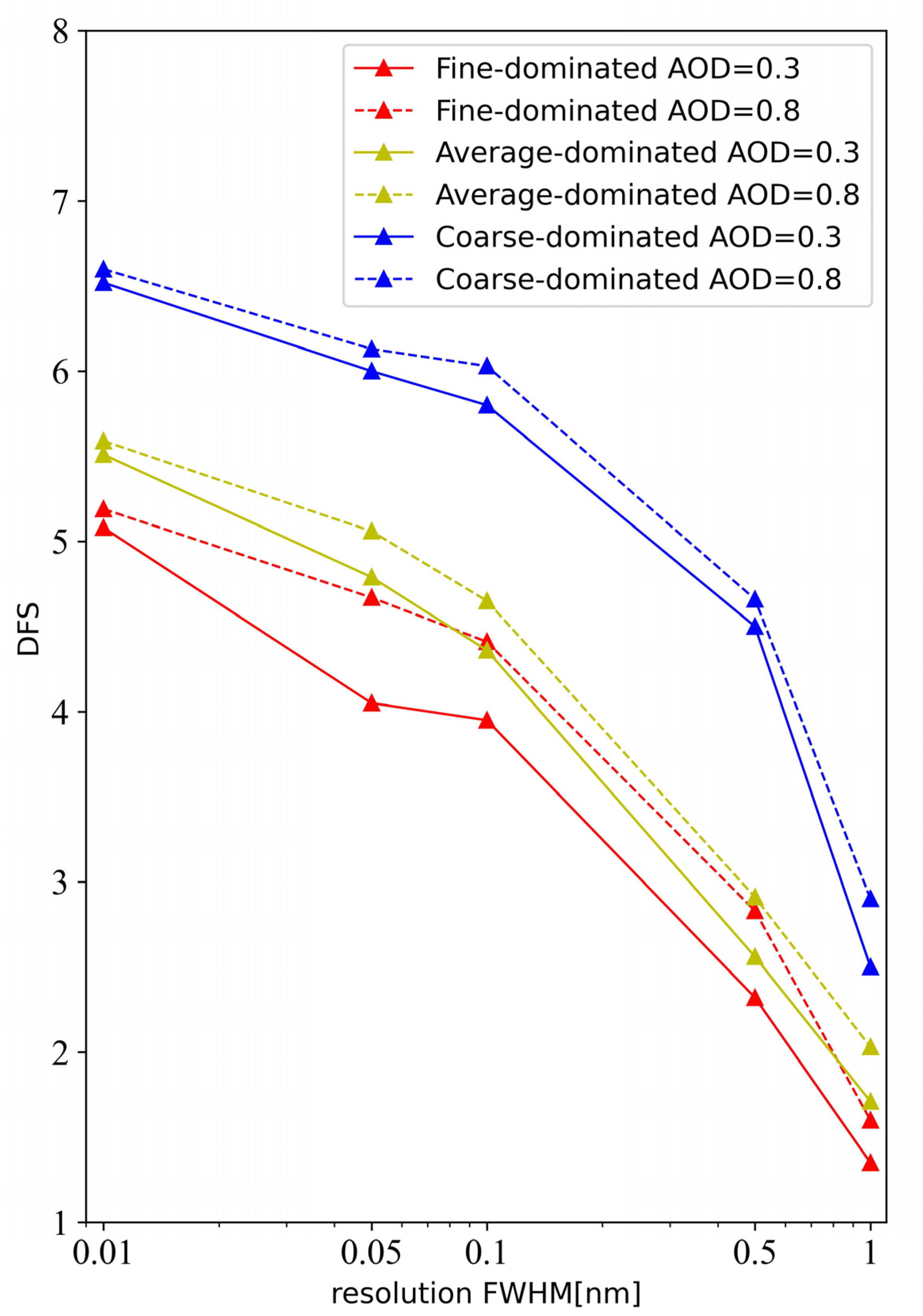
3.2. Spectral Resolution

In order to understand the influence of the spectral resolution of the instrument on the DFS, different spectral resolutions (0.01 nm, 0.05 nm, 0.1 nm, 0.5 nm, and 1 nm) are selected here to simulate from 755 nm to 775 nm while keeping the number of samples constant. To fully express the full content of the O₂ A-band, we calculated the DFS value over the entire range. As shown in Figure 4a, when the instrument resolution is increased from 1 nm to 0.01 nm, the DFS values of the four scenarios have been greatly improved (from 1.2–2.3 increased to 3.8–5.1), because when the spectral resolution is higher, which can contain more information about the vertical distribution of aerosols, the expression of the spectral absorption features in the O₂ A-band would be complete and clear. The aerosol type has little effect on the trend of DFS change with the increase in spectral resolution. Compared with other aerosol types, the DFS value of the ocean-type aerosol is smaller. The ocean type of aerosol has a small optical depth (τ = 0.12) and the aerosol is close to the surface, with a lower boundary layer height (0.5 km).

Here, we examined how ground surface reflectance affects the retrieval aerosol vertical profiles and we fixed the kind of aerosol as biomass burning type, maintaining a steady extinction profile and viewing geometry. The results are shown in Figure 4b. Lower spectral resolution (1 nm) and a higher reflectance (ρ = 0.5) lead to a low DFS value of 1.3. However, the DFS value is raised to 4.6 when the spectral resolution becomes 0.01 nm. It is evident that higher spectral resolution enables the collection of more information. In addition, observing the two datasets of As = 0.3 and As = 0.5, it can be seen that the difference in DFS gets smaller as the spectral resolution goes from 1 nm to 0.01 nm (reduced from 0.45 to 0.05). It is simple to see how high spectral resolution can lessen the reliance on surface reflectance and enhance the retrieval capability of the vertical distribution of aerosols in places with high surface reflectance. The optical principle is shown in Figure 2b. The extinction ability of oxygen in the atmosphere is different at various wavelengths, which means that sunlight of wavelengths in O₂ A-band can penetrate disparate distances in the atmosphere. The spectrum will be degraded, and much aerosol elevation information will be lost when the resolution is too low. As a result, the information obtained by the low-resolution instrument is mixed at different heights in the atmosphere, making the retrieval more dependent on low surface reflectance.

The ratio R of TOA reflectance in the oxygen absorption band and nonabsorption band is generally related to the vertical height of the aerosol, but not to the AOD. As such, the vertical distribution of the aerosol can be retrieved using differential optical absorption spectroscopy (DOAS). Here, △R is used to represent the maximum difference in R between the absorbing band and the nonabsorbing band at different altitudes in the biomass burning aerosol scenarios. When △R approaches 0 and the ratios of TOA reflectance are almost the same, the retrieval cannot be performed regardless of the vertical structure of the aerosol. According to the above conclusions, the retrieval ability of some existing satellites, including the O₂ A-band, can be roughly evaluated according to their spectral ranges and resolutions. The parameters of six typical satellite instruments, including the O₂ A-band, are shown in

Table 2. A partial list of satellite parameters containing oxygen A-bands.

Satellite Name	Launch Year	Spectral Range (nm)	Spectral Resolution	△R
GOME-2	2007	590–790	0.48 nm	0.318
GOSAT	2009	756–775	0.03 nm	0.326
OCO-2	2014	757–775	0.044 nm	0.291
CarbonSat	2018	757–775	0.1 nm	0.268
GF5-B	2021	765–769	0.6 cm−1	0.159

[34,35,36]. GOSAT and OCO-2 have high spectral resolutions, and their spectral ranges can completely cover the O₂ A-band (△R = 0.318,0.326). If the SNR can also meet the retrieval need, the retrieval of the aerosol vertical profiles should be satisfactory. The spectral resolutions of GOME-2 and CarbonSat have no advantage over GOSAT or OCO-2, but the spectral ranges can also cover all O₂ A-bands, so these two satellites can also retrieve within a certain accuracy range (△R = 0.291, 0.268). Although the spectral resolution of GF5-B can meet the need, the spectral range is too narrow. Such a limited spectral range will cause the total DFS value to be too small (△R = 0.158). The spectral range of GF5-B makes it difficult to separate aerosol scattering signals at different heights and is not suitable for retrieving aerosol vertical profiles using the oxygen absorption band.

3.3. Instrument Integration Time

Previously, a fixed value was commonly thought to represent the instrument measurement error. Cheng et al. (2021), for example, chose an absolute error of 0.05 to indicate the instrument measurement error [37]. In general, high-resolution instruments generally have a lower SNR, while low-resolution instruments have a higher SNR. To investigate the effect of instrument SNR and spectral resolution on the total DFS of the complete O₂ A-band, we simulated by altering the different SNR and integration times. Then, we assessed the DFS dependence on SNR and spectral resolution. The abovementioned resolution group was still used for simulation. Taking the urban (highly polluted) aerosol mode as an example, the simulation result is shown in Figure 5. The maximum value of DFS (5.76) appears at the position with a resolution of 0.01 nm and an integration time of 0.6 s. This means that both high resolution and high signal-to-noise ratio can improve the value of DFS for this noise model, but the improvement in DFS from spectral resolution is more obvious. For the lower SNR caused by the integration time, the instrument noise would limit the aerosol vertical information obtained by the oxygen absorption A-band. In addition, the impact of spectral resolution would be weaker than that of high SNR. When the instrument integration time is extended from 0.1 s to 0.6 s, the value of DFS is increased by 13% to 18%. When the resolution is increased from 1 nm to 0.01 nm, the increment of DFS can reach 53% from 41%. This implies that the low spectral resolution instrument causes a greater loss of aerosol vertical profile information. The change trends of DFS of the other three aerosol modes are similar in different integration times and spectral resolutions, although the DFS values are slightly different.

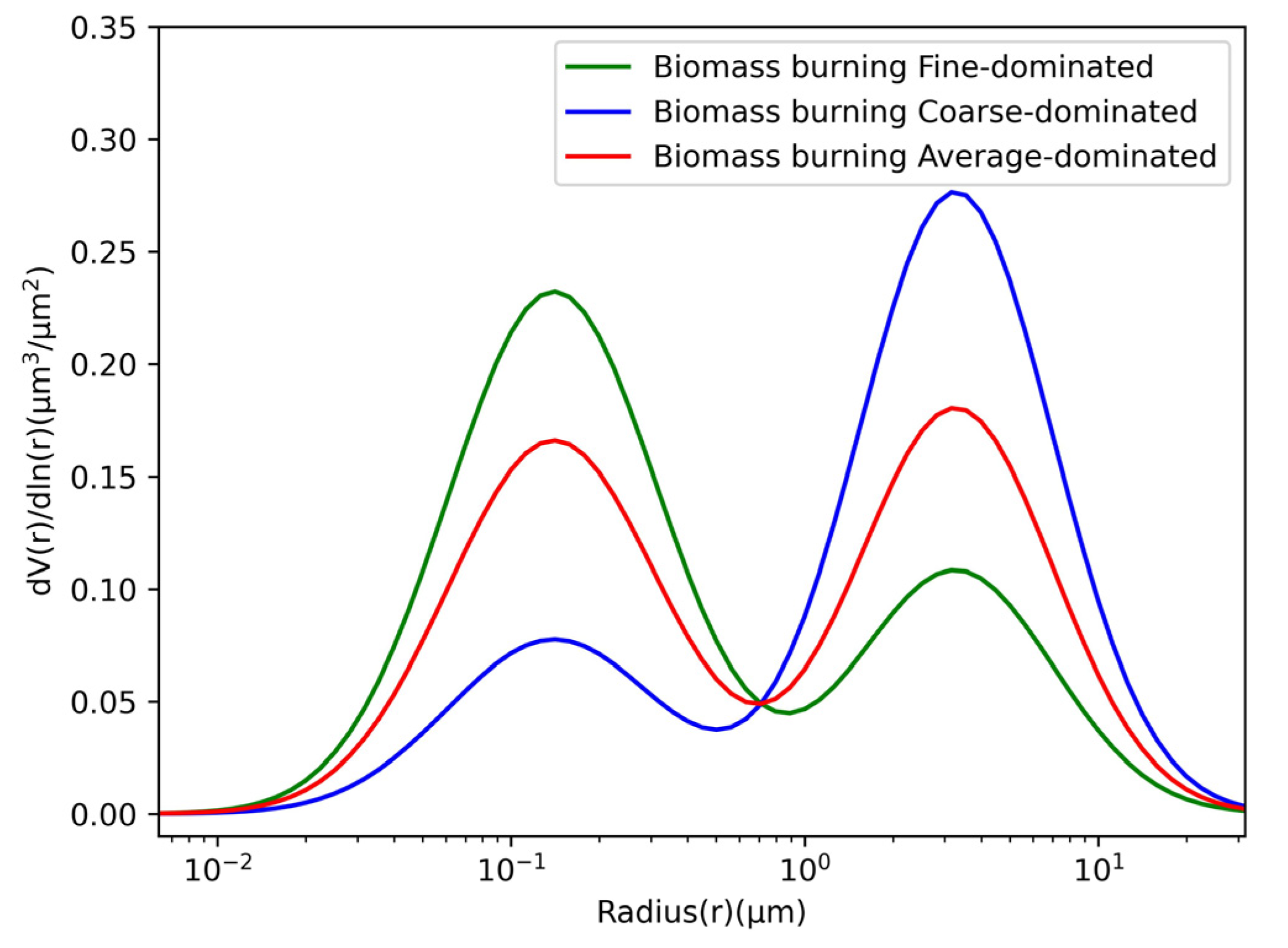
3.4. Volume Size Distribution

Now, we give our consideration to the influence of aerosol size distribution on the relatival of aerosol vertical profile. First, we maintained the aerosol vertical profiles and other optical properties constant. Then, we changed the aerosol column volume ratio from coarse-dominated to fine-dominated. Taking biomass burning aerosol as an example, we set the column volume ratio of fine-dominated to remain unchanged, the ratio of average-dominated to 0.5, and the ratio of coarse-dominated to 0.8. The size distribution of the three aerosol modes mentioned above is shown in Figure 6.

The simulation results are shown in Figure 7, which shows the DFS of three different particle size distributions at different spectral resolutions, where the dotted line is the result of increasing the optical depth in the same simulation conditions. The figure shows that aerosol particle size has a huge impact on the value of DFS. When the size distribution gradually changes from fine-dominated mode to coarse-dominated mode and the AOD is unchanged and remained at 0.3, the DFS value increased from 1.35–5.8 to 2.51–6.52. For the AOD of 0.8, DFS values vary from 1.6–5.19 to 2.89–6.61. The DFS value of the coarse-dominated aerosol is about 20% higher than that of the fine-dominated aerosol. This means that the relatival of aerosol vertical profiles is more sensitive with larger particles in the O₂ A-band. The coarse-dominated aerosol mode measured by instruments has more information and a better retrieval effect. Absorption and scattering intensities of aerosol behave differently owing to the direct effect of aerosol particle size on phase function distribution. In addition, increasing the spectral resolution has a similar effect on retrieval with different aerosol size distributions, and the total DFS improvement is about 3. Therefore, if an accurate assumption of aerosol type and its physical parameters can be made before retrieval, the retrieval accuracy could be improved. Furthermore, the bigger the AOD is, the larger the value of DFS would be regardless of any resolution, which is consistent with the conclusion of previous analyses.

3.5. Prior Error

To explore the effect of prior error and spectral resolution on retrieval, the DFS and posterior error values of different spectral resolutions and different prior errors in the same aerosol mode were simulated here. We set the diagonal elements of the error matrix to the same value to represent the overall relative error of the aerosol extinction profile. Figure 8a describes the function of total DFS of urban–industrial and mixed aerosols as a function of spectral resolution in different prior errors. As shown in the figure, increasing the spectral resolution can increase the total amount of information. When the error matrix’s diagonal value increases from 0.1 to 0.8, the total DFS value increases from 1.89–3.65 to 2.34–5.65. In addition, DFS decreases when prior knowledge shows an increasing trend (the relative error is small), because more prior knowledge limits the acquisition of information according to optimum estimating theory.

Prior knowledge of the aerosol vertical profiles is represented by the covariance matrix, and the ratio of the state vector to the true value can be described by the posterior error covariance matrix. The smaller the posterior error, the more information can be observed. We fixed the prior error and then simulated the posterior error at different spectral resolutions. The simulation results are shown in Figure 8b. The abscissa in the figure represents the relative prior error, and the comprehensive coordinate represents the relative posterior error. The pattern columns in the figure show the relative posterior error reduction value. As can be observed from the figure, the relative posterior error decreases as the spectral resolution increases, which also shows that increasing the spectral resolution helps to obtain more information.

4. Conclusions

This study analyzes the effect of various factors in the O₂ A-band affecting the retrieval capability of aerosol vertical profiles. In order to identify the suitable instruments and retrieval scenarios, the DFS of the O₂ A-band has been simulated. We have used the UNL radiative transfer model to simulate four vertical profile aerosol modes and quantitatively analyzed the influence of various factors on the DFS value. The main conclusions of the paper can be summarized as follows.

• Different viewing geometries will affect the acquisition of aerosol vertical profile information. When the scattering angle is small, the sensitivity of the measurement information to the aerosol profile increases and more information can be obtained. As the scattering angle decreases, the DFS value of the single absorption band increases to about 0.4. Different aerosol modes are affected by the viewing geometry in the same trend.
• Increasing the spectral resolution of the instrument can increase the observed content of information. When the instrument spectral resolution was increased from 1 nm to 0.01 nm, the total DFS value of the O₂ A-band increased from 1.2–2.3 to 3.8–5.1. In addition, increasing the spectral resolution reduces the dependence on the reflectance of the high surface reflectance area during retrieval of the aerosol vertical profiles.
• We simulated the DFS values in different SNR and spectral resolutions by changing the instrument integration time. The results show that more information content can be acquired with the increase in spectral resolution and SNR. The integration time increases the DFS value from 13% to 28%, while spectral resolutions can boost the DFS value (from 41% to 53%). Extending the integration time would increase the DFS value gradually from 13% to 28%. It shows that the spectral resolution has a greater impact on the DFS.
• The retrieval effect of the vertical coarse-dominated aerosol profile in the O₂ A-band is much better, and the DFS value is about 21% higher than the result of the fine-dominated aerosol. However, increasing the spectral resolution has a similar effect on retrieval of aerosol vertical profiles in three size distribution modes.
• Higher spectral resolution of any prior errors can increase the content of information. Concurrently, the reduction of the posterior error also illustrates the improvement in spectral resolution on the DFS.

In general, increasing the spectral resolution of the instrument has a significant effect on the information acquisition of the entire O₂ A-band. The better spectral resolution can also have special advantages in certain situations, such as high-reflectivity ground surface and large prior errors. We maintain that using an instrument with high spectral resolution in the O₂ A-band to further detect and characterize aerosol information can provide valuable supplements to the existing satellite observations, while existing instruments such as EPCI and OCO-2 can retrieve the vertical distribution of aerosols within a certain range of precision. Our work can provide theoretical support for future hyperspectral instruments and algorithm design using the O₂ A-band. Other influencing factors (such as temperature distribution and polarization measurement) will be discussed in future research.

References

1. Shiraiwa, M.; Ueda, K.; Pozzer, A.; Lammel, G.; Kampf, C.J.; Fushimi, A.; Enami, S.; Arangio, A.M.; Frohlich-Nowoisky, J.; Fujitani, Y.; et al. Aerosol Health Effects from Molecular to Global Scales. Environ. Sci. Technol. 2017, 51, 13545–13567. [Google Scholar] [CrossRef] [PubMed]
2. Samset, B.H.; Myhre, G.; Schulz, M.; Balkanski, Y.; Bauer, S.; Berntsen, T.K.; Bian, H.; Bellouin, N.; Diehl, T.; Easter, R.C.; et al. Black carbon vertical profiles strongly affect its radiative forcing uncertainty. Atmos. Chem. Phys. 2013, 13, 2423–2434. [Google Scholar] [CrossRef]
3. Kaufman, Y.J.; Tanre, D.; Boucher, O. A satellite view of aerosols in the climate system. Nature 2002, 419, 215–223. [Google Scholar] [CrossRef] [PubMed]
4. Huang, J.; Adams, A.; Wang, C.; Zhang, C. Black Carbon and West African Monsoon precipitation: Observations and simulations. Ann. Geophys. 2009, 27, 4171–4181. [Google Scholar] [CrossRef]
5. Geddes, A.; Bosch, H. Tropospheric aerosol profile information from high-resolution oxygen A-band measurements from space. Atmos. Meas. Tech. 2015, 8, 859–874. [Google Scholar] [CrossRef]
6. Zeng, Z.C.; Natraj, V.; Xu, F.; Pongetti, T.J.; Shia, R.L.; Kort, E.A.; Toon, G.C.; Sander, S.P.; Yung, Y.L. Constraining Aerosol Vertical Profile in the Boundary Layer Using Hyperspectral Measurements of Oxygen Absorption. Geophys. Res. Lett. 2018, 45, 10772–10780. [Google Scholar] [CrossRef]
7. Rosen, J.M.; Hofmann, D.J. Stratospheric aerosol measurements II: The worldwide distribution. J. Atmos. Sci. 1975, 32, 1457–1462. [Google Scholar] [CrossRef]
8. Amodeo, A.; Pappalardo, G.; Bosenberg, J.; Ansmann, A.; Apituley, A.; Alados-Arboledas, L.; Balis, D.; Bockmann, C.; Chaikovsky, A.; Comeron, A.; et al. A European research infrastructure for the aerosol study on a continental scale: EARLINET-ASOS. In Proceedings of the Conference on Remote Sensing of Clouds and the Atmosphere XII, Florence, Italy, 17–19 September 2007. [Google Scholar]
9. Winker, D.M.; Pelon, J.; Coakley, J.A.; Ackerman, S.A.; Charlson, R.J.; Colarco, P.R.; Flamant, P.; Fu, Q.; Hoff, R.M.; Kittaka, C.; et al. THE CALIPSO MISSION A Global 3D View of Aerosols and Clouds. Bull. Am. Meteorol. Soc. 2010, 91, 1211–1229. [Google Scholar] [CrossRef]
10. Ntwali, D.; Dubache, G.; Ogou, F.K. Vertical Profile Comparison of Aerosol and Cloud Optical Properties in Dominated Dust and Smoke Regions over Africa Based on Space-Based Lidar. Atmos. Clim. Sci. 2022, 12, 588–602. [Google Scholar] [CrossRef]
11. Wu, L.H.; Hasekamp, O.; van Diedenhoven, B.; Cairns, B.; Yorks, J.E.; Chowdhary, J. Passive remote sensing of aerosol layer height using near-UV multiangle polarization measurements. Geophys. Res. Lett. 2016, 43, 8783–8790. [Google Scholar] [CrossRef]
12. Nelson, D.L.; Garay, M.J.; Kahn, R.A.; Dunst, B.A. Stereoscopic Height and Wind Retrievals for Aerosol Plumes with the MISR INteractive eXplorer (MINX). Remote Sens. 2013, 5, 4593–4628. [Google Scholar] [CrossRef]
13. Fischer, H.; Birk, M.; Blom, C.; Carli, B.; Carlotti, M.; Von Clarmann, T.; Delbouille, L.; Dudhia, A.; Ehhalt, D.; Endemann, M. MIPAS: An instrument for atmospheric and climate research. Atmos. Chem. Phys. 2008, 8, 2151–2188. [Google Scholar] [CrossRef]
14. Dubuisson, P.; Frouin, R.; Dessailly, D.; Duforet, L.; Leon, J.F.; Voss, K.; Antoine, D. Estimating the altitude of aerosol plumes over the ocean from reflectance ratio measurements in the O2 A-band. Remote Sens. Environ. 2009, 113, 1899–1911. [Google Scholar] [CrossRef]
15. Stam, D.M.; De Haan, J.F.; Hovenier, J.W.; Aben, I. Detecting radiances in the O2 A band using polarization-sensitive satellite instruments with application to the Global Ozone Monitoring Experiment. J. Geophys. Res. Atmos. 2000, 105, 22379–22392. [Google Scholar] [CrossRef]
16. Wang, P.; Stammes, P.; Van Der A, R.; Pinardi, G.; Van Roozendael, M. FRESCO+: An improved O2 A-band cloud retrieval algorithm for tropospheric trace gas retrievals. Atmos. Chem. Phys. 2008, 8, 6565–6576. [Google Scholar] [CrossRef]
17. Natraj, V.; Spurr, R.J.D.; Boesch, H.; Jiang, Y.B.; Yung, Y.L. Evaluation of errors from neglecting polarization in the forward modeling of O2 A band measurements from space, with relevance to CO2 column retrieval from polarization-sensitive instruments. J. Quant. Spectrosc. Radiat. Transf. 2007, 103, 245–259. [Google Scholar] [CrossRef]
18. Ding, S.G.; Wang, J.; Xu, X.G. Polarimetric remote sensing in oxygen A and B bands: Sensitivity study and information content analysis for vertical profile of aerosols. Atmos. Meas. Tech. 2016, 9, 2077–2092. [Google Scholar] [CrossRef]
19. Chen, X.; Xu, X.G.; Wang, J.; Diner, D.J. Can multi-angular polarimetric measurements in the oxygen-A and B bands improve the retrieval of aerosol vertical distribution? J. Quant. Spectrosc. Radiat. Transf. 2021, 270, 21. [Google Scholar] [CrossRef]
20. Hollstein, A.; Fischer, J. Retrieving aerosol height from the oxygen A band: A fast forward operator and sensitivity study concerning spectral resolution, instrumental noise, and surface inhomogeneity. Atmos. Meas. Tech. 2014, 7, 1429–1441. [Google Scholar] [CrossRef]
21. Nanda, S.; de Graaf, M.; Veefkind, J.P.; ter Linden, M.; Sneep, M.; de Haan, J.; Levelt, P.F. A neural network radiative transfer model approach applied to the Tropospheric Monitoring Instrument aerosol height algorithm. Atmos. Meas. Tech. 2019, 12, 6619–6634. [Google Scholar] [CrossRef] [Green Version]
22. Xu, X.; Wang, J. UNL-VRTM, a testbed for aerosol remote sensing: Model developments and applications. In Springer Series in Light Scattering; Springer: Berlin/Heidelberg, Germany, 2019; pp. 1–69. [Google Scholar]
23. Hou, W.; Wang, J.; Xu, X.; Reid, J.S.; Han, D. An algorithm for hyperspectral remote sensing of aerosols: 1. Development of theoretical framework. J. Quant. Spectrosc. Radiat. Transf. 2016, 178, 400–415. [Google Scholar] [CrossRef]
24. Bernardo, J.M.; Smith, A.F. Bayesian Theory; John Wiley & Sons: Hoboken, NJ, USA, 2009; Volume 405. [Google Scholar]
25. Rodgers, C.D. Inverse Methods for Atmospheric Sounding: Theory and Practice; World scientific: Singapore, 2000; Volume 2. [Google Scholar]
26. Colosimo, S.F.; Natraj, V.; Sander, S.P.; Stutz, J. A sensitivity study on the retrieval of aerosol vertical profiles using the oxygen A-band. Atmos. Meas. Tech. 2016, 9, 1889–1905. [Google Scholar] [CrossRef]
27. Liu, P.F.; Zhao, C.S.; Zhang, Q.; Deng, Z.Z.; Huang, M.Y.; Ma, X.C.; Tie, X.X. Aircraft study of aerosol vertical distributions over Beijing and their optical properties. Tellus Ser. B-Chem. Phys. Meteorol. 2009, 61, 756–767. [Google Scholar] [CrossRef]
28. Schafer, J.S.; Eck, T.F.; Holben, B.N.; Thornhill, K.L.; Anderson, B.E.; Sinyuk, A.; Giles, D.M.; Winstead, E.L.; Ziemba, L.D.; Beyersdorf, A.J.; et al. Intercomparison of aerosol single-scattering albedo derived from AERONET surface radiometers and LARGE in situ aircraft profiles during the 2011 DRAGON-MD and DISCOVER-AQ experiments. J. Geophys. Res. Atmos. 2014, 119, 7439–7452. [Google Scholar] [CrossRef]
29. Baidar, S.; Oetjen, H.; Coburn, S.; Dix, B.; Ortega, I.; Sinreich, R.; Volkamer, R. The CU Airborne MAX-DOAS instrument: Vertical profiling of aerosol extinction and trace gases. Atmos. Meas. Tech. 2013, 6, 719–739. [Google Scholar] [CrossRef]
30. Kipling, Z.; Stier, P.; Johnson, C.E.; Mann, G.W.; Bellouin, N.; Bauer, S.E.; Bergman, T.; Chin, M.; Diehl, T.; Ghan, S.J.; et al. What controls the vertical distribution of aerosol? Relationships between process sensitivity in HadGEM3-UKCA and inter-model variation from AeroCom Phase II. Atmos. Chem. Phys. 2016, 16, 2221–2241. [Google Scholar] [CrossRef]
31. Moorthy, K.K.; Nair, V.S.; Babu, S.S.; Satheesh, S.K. Spatial and vertical heterogeneities in aerosol properties over oceanic regions around India: Implications for radiative forcing. Q. J. R. Meteorol. Soc. 2009, 135, 2131–2145. [Google Scholar] [CrossRef]
32. Dubovik, O.; Holben, B.; Eck, T.F.; Smirnov, A.; Kaufman, Y.J.; King, M.D.; Tanre, D.; Slutsker, I. Variability of absorption and optical properties of key aerosol types observed in worldwide locations. J. Atmos. Sci. 2002, 59, 590–608. [Google Scholar] [CrossRef]
33. Zeng, J.; Xu, X.G.; Wang, J.; Wang, Y.; Chen, X.; Lu, Z.D.; Torres, O.; Reid, J.S.; Miller, S.D. Detecting layer height of smoke aerosols over vegetated land and water surfaces via oxygen absorption bands: Hourly results from EPIC/DSCOVR in deep space. In Proceedings of the IEEE International Geoscience and Remote Sensing Symposium (IGARSS), Electr Network, Waikoloa, HI, USA, 26 September–2 October 2020; pp. 5588–5591. [Google Scholar]
34. Hamazaki, T.; Kaneko, Y.; Kuze, A.; Kondo, K. Fourier transform spectrometer for greenhouse gases observing satellite (GOSAT). In Proceedings of the Enabling Sensor and Platform Technologies for Spaceborne Remote Sensing, Honolulu, HI, USA, 11 January 2005; pp. 73–80. [Google Scholar]
35. Wunch, D.; Wennberg, P.O.; Osterman, G.; Fisher, B.; Naylor, B.; Roehl, C.M.; O’Dell, C.; Mandrake, L.; Viatte, C.; Kiel, M. Comparisons of the orbiting carbon observatory-2 (OCO-2) X CO2 measurements with TCCON. Atmos. Meas. Tech. 2017, 10, 2209–2238. [Google Scholar] [CrossRef]
36. Velazco, V.A.; Buchwitz, M.; Bovensmann, H.; Reuter, M.; Schneising, O.; Heymann, J.; Krings, T.; Gerilowski, K.; Burrows, J.P. Towards space based verification of CO2 emissions from strong localized sources: Fossil fuel power plant emissions as seen by a CarbonSat constellation. Atmos. Meas. Tech. 2011, 4, 2809–2822. [Google Scholar] [CrossRef] [Green Version]
37. Cheng, L.; Shi, W.; Xia, G.; Wang, J.; Chen, Q.; Jin, S. Information content analysis and sensitivity of retrieval of aerosol vertical profiles using polarimetric oxygen A-band spectra. J. Atmos. Environ. Opt. 2022, 17, 360–368. [Google Scholar]
Figure 1. The four aerosol vertical profiles.
Remotesensing 15 00948 g001
Figure 2. (a) DFS of individual channels in O2 A-band (b) Spectral absorption optical depth of atmosphere in the O2 A-band.
Remotesensing 15 00948 g002
Figure 3. DFS of aerosol vertical profiles for different geometry: (ac) VZA = 15°,45°, 75° and (cf) DFS of different aerosol vertical profiles for identical geometry.
Remotesensing 15 00948 g003
Figure 4. Influence of spectral resolution on DFS value: (a) DFS of four aerosol vertical profiles for different spectral resolutions; (b) DFS of biomass burning aerosol for different spectral resolutions and ground surface reflectivity.
Remotesensing 15 00948 g004
Figure 5. Influence of spectral resolution and integration time on DFS values of four aerosol vertical profiles.
Remotesensing 15 00948 g005
Figure 6. The size distribution of three aerosol modes.
Remotesensing 15 00948 g006
Figure 7. The influence of three aerosol size distributions on DFS value at different spectral resolutions.
Remotesensing 15 00948 g007
Figure 8. Influence of the prior error of aerosol vertical profiles for different spectral resolutions of urban–industrial and mixed aerosols: (a) influence on DFS values; (b) influence on posterior error.
Remotesensing 15 00948 g008