Technical Note

A Novel Deep Learning Model for Mining Nonlinear Dynamics in Lake Surface Water Temperature Prediction

1
College of Atmospheric Sciences, Lanzhou University, Lanzhou 730000, China
2
Laboratory of Applied Mathematics and Complex Systems, Center for Data Science, School of Mathematics and Statistics, Lanzhou University, Lanzhou 730000, China
3
Institute for Learning Sciences & Teacher Education, Australian Catholic University, Brisbane 4001, Australia
4
Frontiers Science Center for Deep Ocean Multispheres and Earth System, Key Lab of Submarine Geosciences and Prospecting Techniques, MOE and College of Marine Geosciences, Ocean University of China, Qingdao 266100, China
*
Author to whom correspondence should be addressed.
Remote Sens. 2023, 15(4), 900; https://doi.org/10.3390/rs15040900
Submission received: 29 November 2022 / Revised: 25 January 2023 / Accepted: 3 February 2023 / Published: 6 February 2023
(This article belongs to the Special Issue Machine Learning for Spatiotemporal Remote Sensing Data)

Abstract

:
As one of the critical indicators of the lake ecosystem, the lake surface water temperature is an important indicator for measuring lake ecological environment. However, there is a complex nonlinear relationship between lake surface water temperature and climate variables, making it difficult to accurately predict. Fortunately, satellite remote sensing provides a wealth of data to support further improvements in prediction accuracy. In this paper, we construct a new deep learning model for mining the nonlinear dynamics from climate variables to obtain more accurate prediction of lake surface water temperature. The proposed model consists of the variable correlation information module and the temporal correlation information module. The variable correlation information module based on the Self-Attention mechanism extracts key variable features that affect lake surface water temperature. Then, the features are input into the temporal correlation information module based on the Gated Recurrent Unit (GRU) model to learn the temporal variation patterns. The proposed model, called Attention-GRU, is then applied to lake surface water temperature prediction in Qinghai Lake, the largest inland lake located in the Tibetan Plateau region in China. Compared with the seven baseline models, the Attention-GRU model achieved the most accurate prediction results; notably, it significantly outperformed the Air2water model which is the classic model for lake surface water temperature prediction based on the volume-integrated heat balance equation. Finally, we analyzed the factors influencing the surface water temperature of Qinghai Lake. There are different degrees of direct and indirect effects of climatic variables, among which air temperature is the dominant factor.

Graphical Abstract

1. Introduction

Lake surface water temperature (LSWT) is one of the important indicators of lake ecosystems. Some research on global warming reported the LSWT of global lakes shows a general warming trend, and this trend is expected to continue in the future [1,2,3]. Warming surface water temperatures would reduce the ice cover and shorten the lake’s icing period. The decrease of ice cover and the increase of LSWT would change the mixing regimes of the lake and further affect the exchange of nutrients and oxygen [4]. In addition, changes in LSWT would affect lake water quality, according to the previous study [5]. This series of changes will have a serious impact on the lake’s ecological environment, affect lake biodiversity, and bring ecological and economic impacts to human society. Therefore, it is crucial to accurately predict future changes in LSWT. However, changes in LSWT is the result of the interaction of multiple climate variables [6], and complex nonlinear relationships exist between climate variables and LSWT, which poses difficulties for accurate prediction. We established a new deep learning model to mine the nonlinear dynamics in the prediction of LSWT to achieve more accurate prediction results and applied the model to the prediction of lake surface water temperature of Qinghai Lake.
Currently, the main statistical-related methods for predicting LSWT can be divided into three categories: hybrid physical-statistical models, traditional statistical models, and machine learning models. Firstly, the physically-statistically based Air2water model [7,8,9,10,11], is a very popular model and has achieved the best results of several studies [12,13]. It is a simple and accurate model based on the volume-integrated heat balance equation, and using only air temperature as an input [14]. Secondly, traditional statistics-based regression models are also frequently used in the prediction of LSWT [15,16,17]. Thirdly, machine learning algorithms have flourished in recent years and are also commonly used to solve water temperature predictions in lakes and rivers [18], such as Random Forests, M5Tree models [12], and Multi-Layer perceptron (MLP) [12,13,19,20]. To further improve the accuracy, researchers have combined various machine learning models to form new frameworks [21], or combining MLP with wavelet variation [13,22,23], which is commonly used to improve the accuracy of hydrologic time series analysis [24]. In addition, lake model is the main method to simulate lake water temperature. For example, the Freshwater Lake model (FLlake) [25] is a commonly used one-dimensional lake model which can simulate the thermal behavior and vertical temperature structure of lake surface at different depths. In this model, the lake is divided into a mixed layer and a thermocline layer according to thermal structure, and the thermocline temperature profile is parameterized based on self-similarity theory [26]. Recent studies have conducted sensitivity experiments and calibration on Qinghai Lake to improve the accuracy of lake temperature simulation by FLlake model [27].
Deep learning shows a stronger ability to handle large data and complex problems than traditional methods. LSWT prediction is essentially a time series prediction problem. There are many deep learning models for time series prediction that have been applied to various domains. The classical model of time series prediction problem in deep learning is Recurrent Neural Network (RNN) [28], which can capture the pattern of data changes over time well. However, the RNN has difficulty in learning the long-term dependencies of time series. Then, the Long Short-Term Memory network (LSTM) model alleviates this problem to some extent [29]. In the weighted average temperature prediction problem, LSTM achieved better prediction results than RNN in the experiment [
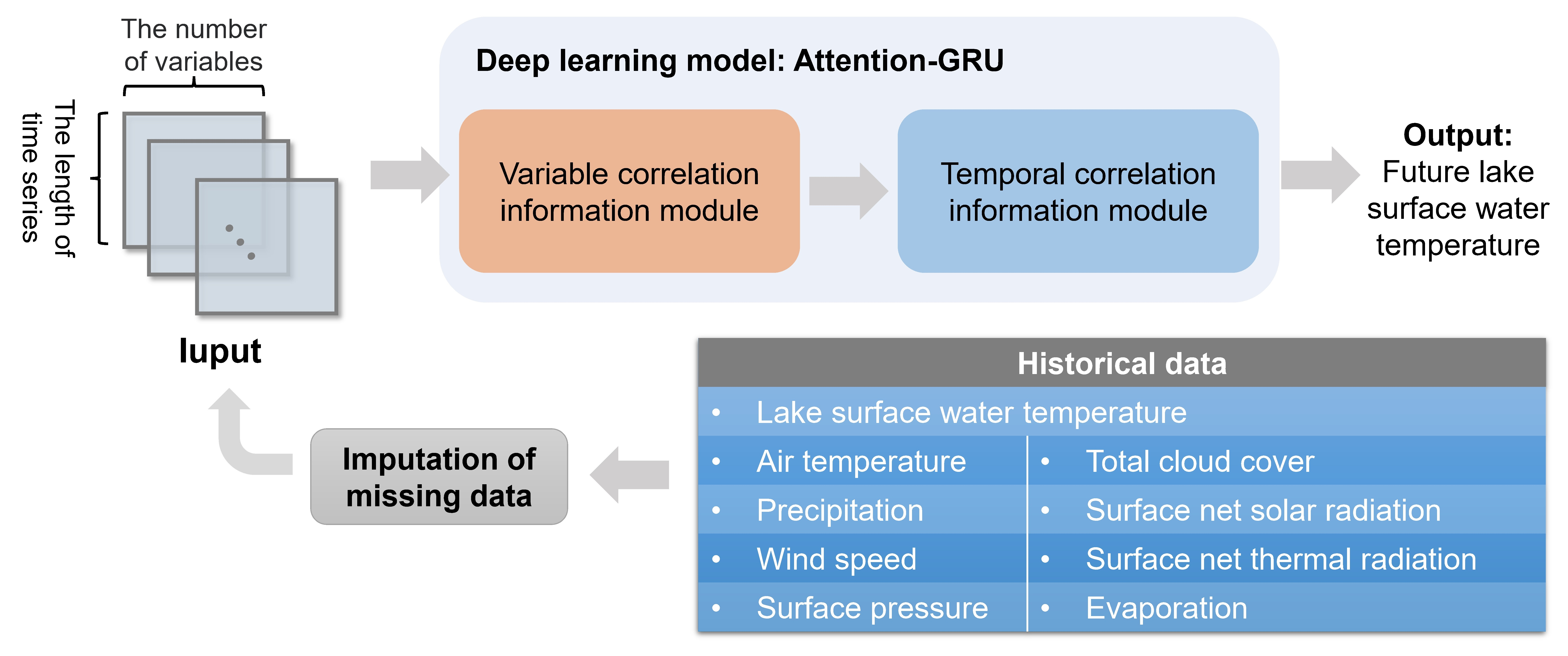
30]. Subsequently, the Gated Recurrent Unit (GRU) model further improves the LSTM, which achieves similar results with fewer model parameters [31]. Another structure in deep learning, the Attention mechanism [31,32], has been the focus of many researchers. In the prediction of ocean surface temperature, a model incorporating the Attention mechanism in the GRU encoder–decoder structure was applied [33]. With the development of the Attention mechanism, the Transformer model was proposed and has become one of the most popular deep learning models, while the Self-Attention mechanism [34] was also proposed. The GTN [35] model uses the Self-Attention mechanism to construct a two-tower Transformer model, which effectively extracts time-related and channel-related features in multivariate time series, respectively.
The Air2water model uses only air temperature as a direct input. However, air temperature is the main factor affecting surface water temperature in lakes, not the only factor [
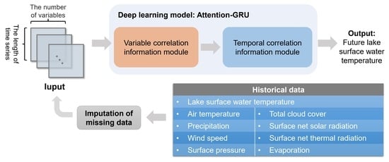
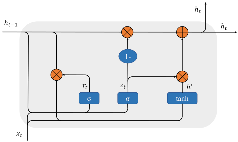
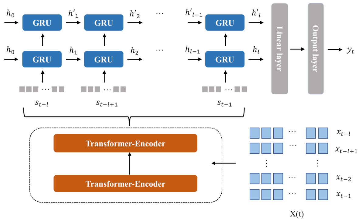
36]. This allows the Air2water model to discard some information that affects the variability of lake surface water temperature. Fortunately, we have access to many satellite observations and meteorological station data, through which we can obtain more information on climate variables. How to construct the model to extract effective features from the data is the key. Given the superiority of deep learning in extracting effective features from complex nonlinear relationships compared with traditional statistical methods, we would construct a new deep learning model for predicting LSWT to obtain more accurate prediction results. The interaction of climate variables and temporal autocorrelation are the two main aspects that contribute to the variation of LSWT. It is crucial to effectively extract data features from both aspects using deep learning models. Inspired by the GTN model [
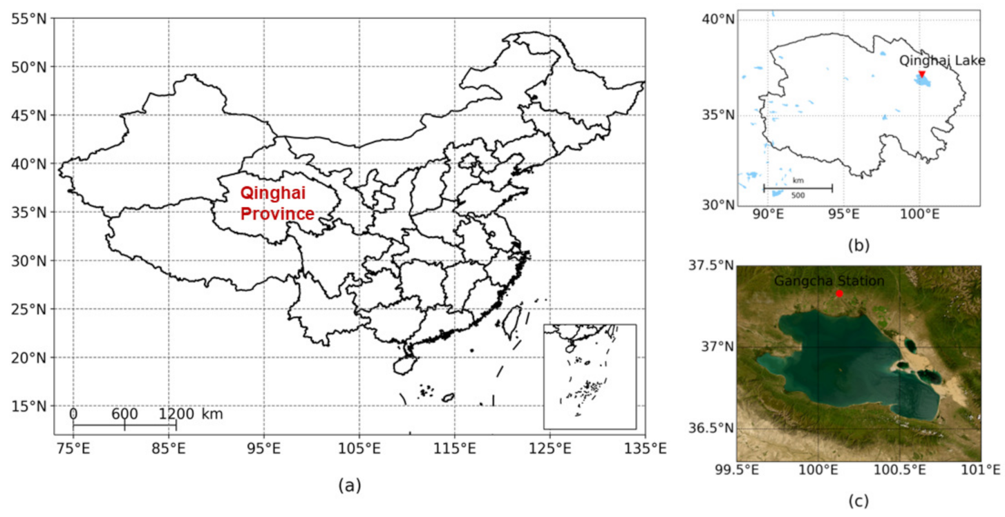
35], the information in the multivariate time series is divided into two parts: variable correlation information and temporal correlation information, and the feature extraction module is constructed separately. In the variable correlation information module, the Self-attention mechanism is used to extract the key variable features. In the module of temporal correlation information, the GRU model is used to capture the changing laws of time series. The two modules are combined to form the Attention-GRU model. To verify the validity of the model, we apply the proposed model to a case study of lake surface water temperature prediction in Qinghai Lake and compare it with seven benchmark models. Qinghai Lake is the largest inland lake in China, which plays an irreplaceable role in regulating climate and maintaining the ecological balance in the northwestern part of the Qinghai–Tibet Plateau. The prediction of lake surface water temperature in Qinghai Lake is of great significance for protecting ecological environment. However, due to the complex physical processes that are difficult to describe accurately there is still a space for improvement in the prediction of lake surface water temperature of Qinghai Lake. We build a deep learning model to make full use of the large amount of information, explore the non-linear relationships among different climate variables and try to to improve the prediction by mining the dynamical system behind the data. Meanwhile, by calculating the partial correlation coefficient, the influencing factors of the LSWT in Qinghai Lake are discussed in the Section 5.1. The main contributions are as follows:
(1)
A novel deep learning model (Attention-GRU) for surface water temperature prediction is established. The proposed model outperforms the Air2water model in surface water temperature prediction for Qinghai Lake and achieves the best prediction results, which indicates that the proposed model can mine the nonlinear dynamics of the research problem.
(2)
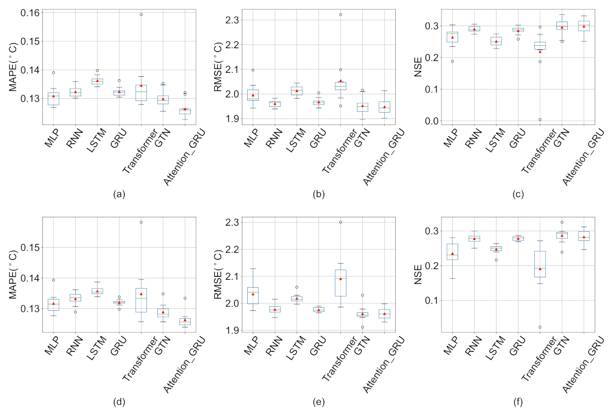
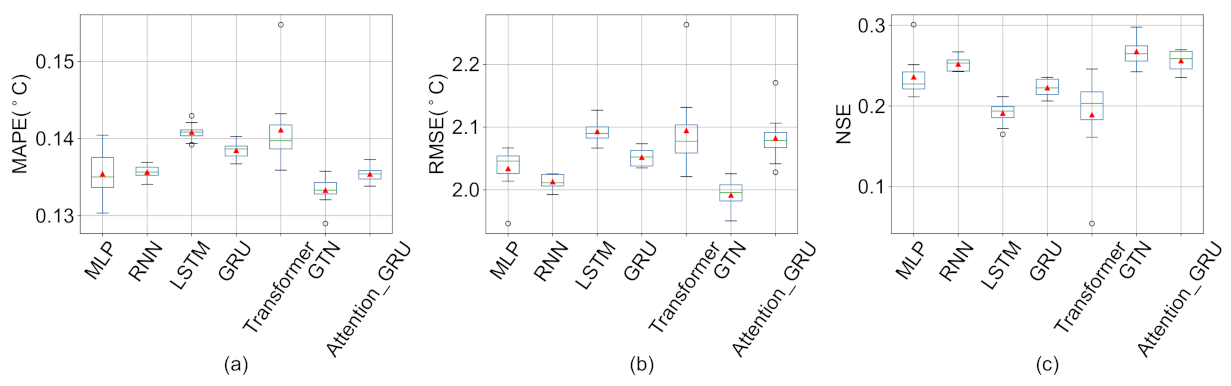
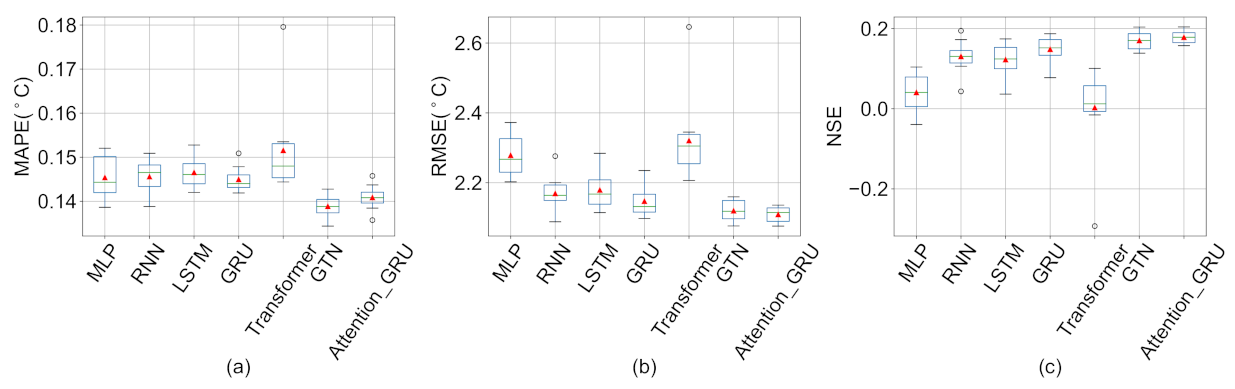
We show the results of ten experiments with each deep learning model, indicating that the results of the proposed model are relatively stable, and through ablation experiments, we verify the effectiveness of the proposed model structure.
(3)
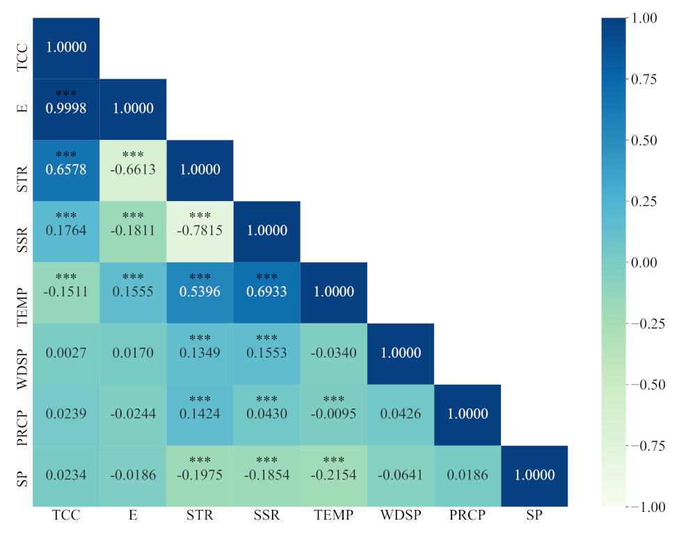
By calculating the partial correlation coefficient, the influencing factors of surface water temperature in Qinghai Lake were analyzed. Climate variables have direct or indirect effects on the surface water temperature of Qinghai Lake in different degrees, and the dominant factor is air temperature.
(4)
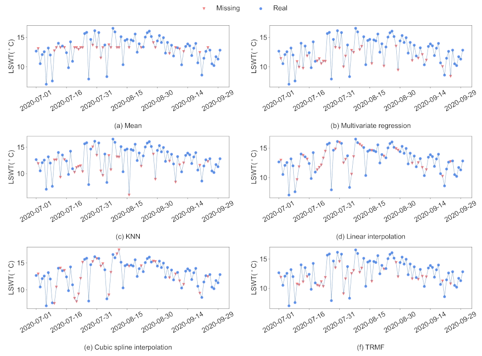
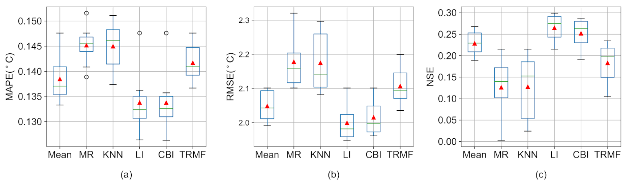
There are a lot of missing values in the LSWT data of Qinghai Lake, and we used six common missing value imputation methods to fill in the missing data. By comparing the filling effects of different missing value imputation methods, the validity of the proposed model on multiple data sets is verified, and the dependence of deep learning models on data quality is shown.
The rest of the paper is organized as follows. Section 2 presents the model framework and describes the theoretical knowledge of the model in detail. We present the application of the proposed model in Section 3, including the introduction of data sources and description of the experimental procedure. Section 4 analysis of the experimental results. In Section 5, we analyze the factors influencing the LSWT; the impact of the missing value imputation method on the prediction model; the limitations and future work of the proposed model. Finally, Section 6 summarizes the whole paper.

2. A Novel Deep Learning Model: Attention-GRU

2.1. The Preliminaries

This subsection illustrate two basic methods (i.e., the Self-Attention and the GRU) in our proposed model.

2.1.1. The Self-Attention

Self-Attention is the core idea of the Transformer model. The Transformer model was proposed by the Google team and was initially applied to machine translation and achieved the best results [34]. It can learn the correlation between variables and extract important factors. To begin this process, there are three different matrices, namely Query (Q), Key (K), and Value (V), which are calculated by the following formulas:
Q = X ( t ) T W Q ,
K = X ( t ) T W K ,
and
V = X ( t ) T W V ,
where, X t is the input data; W Q , W K and W V are the weight matrices. Then, the product of Q and K is processed using the Softmax activation function to obtain a score matrix. Finally, the product of the score matrix and V is calculated as the result of the Self-Attention mechanism as:
Z = Softmax ( Q K T d k ) V ,
where, d k is the column numbers of Q and K. You can think of Softmax ( Q K T Q K T d k d k ) as the similarity of Q and K, and divided by d k for normalization.

2.1.2. The GRU

The Gated Recurrent Unit (GRU) model [31] uses a gating mechanism to control the memory and forgetting of information. At the time t node, the reset gating signal r t and the update gating signal z t are calculated from the current input s t and the hidden state of the previous node h t 1 as:
r t = σ ( W r [ h t 1 , s t ] + b r ) ,
and
z t = σ ( W z [ h t 1 , s t ] + b z ) ,
where, W and b are weight and bias of gate respectively. σ is the sigmoid function that can convert the value between 0 and 1. The gating signal can be understood as the filtering ratio of data information.
After that, use the reset gate signal r t to filter the hidden state of the previous time node h t 1 , and then obtain the reset historical hidden state h t 1 . The current information h is calculated by the reset historical hidden state h t 1 and the current input data s t . Finally, the update gating signal z t is used to selectively forget past information and memorize current information to obtain the hidden state of the current node h t . The above calculation process is as follows:
h t 1 = h t 1 r t ,
h = tanh ( W h [ h t 1 , s t ] + b h ) ,
and
h t = z t h t 1 + ( 1 z t ) h ,
where ⊙ is the Hadamard product, the product of the corresponding positions, and tanh is the activation function. Repeat the above for all time nodes. The structure diagram of GRU is shown in the Figure 1.

2.2. The Proposed Model: Attention-GRU

Lake surface water temperature and related climate variables constitute multivariate time series data. To more comprehensively extract the features of multivariate time series and obtain more accurate prediction results, we successively build a variable correlation information module and a temporal correlation information module in the proposed model (Attention-GRU). The structure of Attention-GRU is shown in Figure 2.
The variable correlation information module encodes variable features, which consists of a two-layer Transform-Encoder structure. The Transform-Encoder structure is mainly composed of the Self-Attention layer and the fully connected layer, and the calculation process is as follows:
Z ( t ) = Self _ Attention ( X ( t ) ) ,
and
S ( t ) = Relu ( W 1 Z ( t ) + b 1 ) W 2 + b 2 ,
where Self _ Attention represents the calculation process of the Self-Attention mechanism, and W and b are the weights and biases. In addition, like the original Transform-Encoder structure, residual connections are added after the regularization of each layer. The temporal information module consists of two-layer GRU, and the input of this module is the embedding ( S ( t ) ) obtained by the variable correlation information module. The output of each time node in the first GRU layer is used as the input of the corresponding time node in the second GRU layer. After splicing the output of the last node of each GRU layer, the final prediction result y t of the model is obtained through full connection calculation as:
y t = w · Contact ( G R U 1 , G R U 2 ) + b ,
where G R U i is the output of the last node of the i t h GRU layer. Contact represents the splicing operation, and w and b are weights and biases, respectively.
The loss function of the model is the L1-Norm loss function, and the calculation formula as:
L 1 = 1 N i = 1 N y i y ^ i ,
where y i is the true value and y ^ i is the predicted result of the model. The pseudocode of the Attention-GRU model is shown in Algorithm 1.
Algorithm 1: Attention-GRU
Remotesensing 15 00900 i001

3. Experiments

3.1. Data Sources

As a climate-sensitive area, the air temperature of the Qinghai–Tibet Plateau continues to rise [37]. The Qinghai–Tibet Plateau is a region with a high density of lake distribution in China, which is relatively sparsely populated, and the environment is less affected by human activities. Studies have shown that Qinghai–Tibet Plateau lakes respond to climate change in several ways, including changes in surface water temperature [38]. The surface water temperature of Qinghai Lake, which is located on the Qinghai–Tibet Plateau, should be of concern. Figure 3 shows the geographical location of Qinghai Lake. It is in the northeastern part of the Qinghai–Tibet Plateau, with a plateau continental climate, about 105 km long and 63 km wide, and the lake surface is 3260 m above sea level. Qinghai Lake is the largest inland lake in China, with an area of about 4300 km 2 and a certain trend of expansion in recent years [39]. It is an important water body for maintaining ecological security in the northeastern part of the Qinghai–Tibet Plateau.
Daily surface water temperature data and related meteorological data of Qinghai Lake from 2000 to 2020 are selected in this study, and the data will be explained in detail in the following. Moderate Resolution Imaging Spectroradiometer (MODIS) is an important instrument used in the US Earth Observing System (EOS) program to observe global biological and physical processes. MODIS data are derived from satellite observations and their products are rich in information, providing a variety of features of the land, ocean, and atmosphere. The data source of LSWT in this paper is MOD11A1 daily surface temperature product [40], which is the MODIS/Terra LST level 3 synthetic products. The product has a spatial resolution of 1 km × 1 km and includes daytime LSWT (LSWT_Day) and nighttime LSWT (LSWT_Night) as well as quality control indexes. After quality control of data according to the quality control index, the daily LSWT sequence of Qinghai Lake is obtained by calculating the average temperature in the Qinghai Lake region. Quality control excludes data points affected by other factors such as clouds, as well as data points with emissivity error greater than 0.04 and LSWT error greater than 2K. Since Qinghai Lake has a icing period, the data measured by satellite when the lake freezes will not be the surface water temperature data of the lake. Therefore, Qinghai Lake in summer (including July (Jul.), August (Aug.) and September (Sep.)) was selected for study to avoid the influence of the icing period. Table 1 describes the detailed information of LSWT of Qinghai Lake.
Relevant meteorological data include daily average air temperature (TEMP), daily average rainfall (PRCP), daily average wind speed (WDSP), and daily average surface pressure (SP) from Guncha meteorological stations (GCS). In addition, there are total cloud cover (TCC), net surface solar radiation (SSR), net surface thermal radiation (STR), and evapotranspiration (E) from the ERA5 reanalysis data. ERA5 is the fifth generation atmospheric reanalysis of global climate data from the European Centre for Medium-Range Weather Forecasts (ECMWF) with a spatial resolution of 0 . 25 × 0 . 25 . For details about the meteorological data, see Table 2.

3.2. Imputation of Missing Data

The missing values of the research data are shown in Table 3. It can be found that the missing values of the data set mainly occur in the LSWT data, with the missing ratio reaching 34.47%. There are a few missing values in other relevant meteorological data. To make full use of the known information, the missing values of LSWT_Day and LSWT_Night of Qinghai Lake were imputed respectively, and then the average value was calculated to obtain the complete LSWT sequence.
Missing values imputation is often the first task of data analysis. After filling in the missing values, the dataset will be more complete, which is convenient for the establishment of subsequent models. At the same time, the quality of imputation often has an impact on the subsequent model effect. Therefore, it is particularly important to select an appropriate imputation method according to data characteristics. In this paper, six commonly used imputation methods for time series are selected to fill missing data, including mean filling, multivariate regression interpolation, KNN, linear interpolation, cubic spline interpolation, and TRMF [41] model based on the matrix decomposition method. Taking the surface water temperature of Qinghai Lake in 2020 as an example, Figure 4 shows the results of each imputation method.

3.3. Experiments Settings

In this study, we use seven days of historical information to make a single-step prediction. When predicting the LSWT at time t ( y t ), the input data X ( t ) are the LSWT and relevant meteorological data of the past seven days (See Appendix B for partial autocorrelation of Qinghai Lake LSWT). x t i = ( x t i 1 , x t i 2 , , x t i D ) ( i = 1 , 2 , , 7 ) is the feature vector at the time t i , and D is the number of features. The X ( t ) is detailed as:
X ( t ) = x t 7 x t 6 x t 1 = x t 7 1 , x t 7 2 , , x t 7 D x t 6 1 , x t 6 2 , , x t 6 D x t 1 1 , x t 1 2 , , x t 1 D .
We select eight benchmark models for comparative experiments. The benchmark models and selection principles are as follows: (1) The classic model for lake surface water temperature prediction: Air2water [7,8,9,10,11]; (2) The commonly used neural network in lake surface water temperature prediction: Multi-Layer perceptron (MLP); (3) Deep learning models commonly used in time series prediction problems: Recurrent Neural Network (RNN) [28], Long Short-Term Memory Network (LSTM) [29] and Gated Recurrent Unit (GRU) [31]; (4) Deep learning models based on Self-Attention mechanism that is a very popular deep learning algorithm: Transformer model [34] and GTN model [35]. In addition, GRU and Transformer models can also be used for ablation experiments. The batch size of all deep learning models is 128, the learning rate is 0.0001, and each model is trained ten times separately. Adam optimizer [42] is used to optimize the training (See Appendix A for additional experimental settings). We divide the research dataset into three parts (Table 4): training set, validation set, and test set. The training set selects the summer data from 2000 to 2014, the validation set selects the summer data from 2015 to 2017, and the remaining summer data from 2018 to 2020 as the test set.

3.4. Evaluation Metric

The evaluation metrics used in this paper include the root mean square error (MAPE), the mean absolute percentage error (RMSE), and the Nash–Sutcliffe coefficient of efficiency (NSE). Their calculation formula is as:
M A P E = 1 N i = 1 N y ^ i y i y i ,
R M S E = 1 N i = 1 N ( y ^ i y i ) 2 ,
and
N S E = 1 i = 1 N y i y ^ i 2 i = 1 N y i y ¯ 2 ,
where, y i is the true value, y ^ i is the predicted result of the model, y ¯ is the average of observations, and N is the number of observation samples. The MAPE and RMSE values are range from 0 , 1 . The smaller the index value of MAPE and RMSE, the more accurate the prediction result. In addition, the value of NSE is range from , 1 . The closer the value of NSE is to 1, the more confident the model is. When the value of NSE is close to 0, it means that the results of the model are close to the mean of the observed values; and when the value is less than 0, the model is less reliable.

4. Results

The experimental results of test sets are shown in Table 5, Table 6 and Table 7, in which the results of deep learning models represent the mean (standard deviation) of ten training results. The bolded numbers represent the best evaluation index values under each missing value imputation method. Most of the best predictions are the results of the Attention-GRU model, which illustrates the effectiveness of the proposed model. For each prediction model, the best predictions are marked with “ * ”, which are mostly obtained by linear interpolation, and a few are produced by cubic spline interpolation. Therefore, the missing value imputation is better with linear interpolation and cubic spline interpolation, and subsequent analyses will also focus on the model prediction effects under these two missing value imputation methods.

4.1. Comparison with Air2water

The Air2water model is a commonly used model to predict lake surface water temperature. Comparing with the Air2water model can better illustrate the validity of the proposed model. By the experimental comparison of the lake surface water temperature prediction in Qinghai Lake, the Attention-GRU model shows the best prediction, with the MAPE index of 0.126, the RMSE index of 1.948, and the NSE index of 0.299. However, in the Air2water model results, the MAPE index value is 0.148, the RMSE index value is 2.102, and the NSE index value is 0.215. Compared to the Air2water model, the MAPE index of the Attention-GRU model is improved by 14.86%, the RMSE index is improved by 7.32%, and the NSE index is improved by 39.07%. Furthermore, as can be seen from Figure 5, in addition to the Attention-GRU model, other deep learning models also produced better results than the Air2water model in most cases.

4.2. Comparison with Other Deep Learning Methods

Figure 6 shows the distribution of ten experimental results for each deep learning model under linear interpolation and Cubic spline interpolation methods (See other missing value imputation methods results in Appendix C). The averages of MAPE, RMSE and NSE indicators of Attention-GRU model with linear interpolation are all the best results among deep learning models. Under cubic spline interpolation, MAPE index of Attention-GRU model is the optimal value, but RMSE index value and NSE index value are like the GTN model. To illustrate the role of each module of the Attention-GRU model, we compare the proposed model with the GRU model and the Transformer model. The average value of each evaluation index of GRU model with linear interpolation is: MAPE index is 0.132, RMSE index is 1.968, and NSE index is 0.285. The average value of each evaluation index of the Transformer model is: MAPE index is 0.135, RMSE index is 2.055, and NSE index is 0.219. Experimental results of the GRU model and the Transformer model are both worse than the Attention-GRU model. Therefore, the model structure of the Attention-GRU model is valid. In addition, the application effect of the GTN model in this study is slightly worse than that of the Attention-GRU model Under linear interpolation. The difference between the proposed model and the GTN model mainly lies in the combination of modules and the model used in the learning of time series variation. It can be said that the combination of the proposed model is more suitable for this study, and the GRU has a stronger ability to capture the time series variation.

5. Discussion

5.1. Analysis of Influencing Factors of Lake Surface Water Temperature

Analysis of the factors influencing the LSWT is essential. Since the LSWT is the result of the combined effect of climate variables, the partial correlation coefficient (pcorr) is used to respond to the magnitude of the effect of each climate variable on the LSWT (Table 8). At the same time, there are interactions between climate variables, and Figure 7 shows the partial correlation coefficients between each climate variable. The main factor that directly affects the LSWT is TEMP (pcorr = 0.515, p-value = 0.000), followed by STR (pcorr = −0.228, p-value = 0.000), E (pcorr = 0.225, p-value = 0.000), TCC (pcorr = −0.220, p-value = 0.000) and SP (pcorr = 0.129, p-value = 0.000) which have a weaker correlation with the LSWT.
The correlation between other climate variables and LSWT is not significant (p-value > 0.05) but can have an indirect effect on LSWT by influencing other climate variables. SSR has a very significant correlation with TEMP (pcorr = 0.714, p-value = 0.000) and STR (pcorr = −0.768, p-value = 0.000). PRCP is correlated with STR (pcorr = 0.201, p-value = 0.000) and SSR (pcorr = 0.125, p-value = 0.000). WDPS is also correlated with STR (pcorr = 0.110, p-value = 0.000) and SSR (pcorr = 0.118, p-value = 0.000). There are different degrees and forms of influence of each meteorological variable on LSWT. The interactions between climate variables make the prediction of LSWT more complex.

5.2. Influence of Imputation Methods on Prediction Results

Figure 8 shows the experimental results of the deep learning model under various missing value interpolation methods, including mean filling (Mean), multivariate regression interpolation (MR), KNN, linear interpolation (LI), cubic spline interpolation (CBI), and TRMF. The experimental results show that the linear interpolation and the cubic spline interpolation are more effective in filling the missing values. Deep learning models are a data-driven approach. Data quality plays an important role in the predictive effectiveness of deep learning models. The quality of the data population determines, to some extent, the average level of prediction performance. When forecasting with poor quality filler data, the best model results cannot exceed the worst model results when using good quality filler data. Therefore, careful missing value imputation is necessary before making predictions.

5.3. Limitations and Future Works

There are still some limitations to our study. First, lakes with different properties respond differently to climate variables, but the model does not take into account lake properties that affect lake temperature, such as water level and lake area. In the future, more indicators will be considered. Secondly, since the proposed model considers the effect of historical data on LSWT, the absence of historical data will affect the prediction accuracy. It is one of the future tasks to improve the missing value processing method and build higher quality datasets. Third, Flake [25] can model the vertical water temperature distribution and the energy budget between different depth layers of the lake and also performs well in the simulation of the LSWT. In contrast to the Flake [25], deep learning models lack the use of physical mechanisms, which are less interpretable. However, deep learning models have strong data mining ability and high computational efficiency, especially when dealing with a large number of complex data problems. Due to the more complete mining of data information, Attention-GRU has higher prediction accuracy. It is able to learn about dynamical systems whose physical mechanisms are not well understood, and the parameterization process in the lake model is avoided. In the future, the model error of the lake model can be further improved by combining the advantages of the lake model and the deep learning model. Moreover, as a statistical model, the deep learning model is more suitable for short-term prediction. Finally, this paper only studies summer surface water temperature predictions for Qinghai Lake, which will be extended to more lakes in the future.

6. Conclusions

In this study, we have proposed an Attention-GRU model for LSWT prediction based on the Self-Attention mechanism and GRU model, and the proposed model successfully mines nonlinear dynamics from the data to obtain more accurate prediction results. In the comparative experiments, the Attention-GRU model has achieved the best prediction results and significantly outperformed the results of the Air2water model. In addition, other deep learning models also have achieved better prediction results than the Air2water model, which verifies the effectiveness of the deep learning model in the prediction of lake surface water temperature. Furthermore, ablation experiments have shown that the proposed model structure is effective, and it is more suitable for the prediction of lake surface water temperature from the perspective of prediction effect. The analysis shows that the various climate variables interact with each other and have direct or indirect effects on the LSWT of Qinghai Lake. At the same time, LSWT also has a temporal correlation. The proposed model takes advantage of different modules to learn the information about the climate variables interaction and time series correlation, which can more sufficiently mine the effective nonlinear correlation information in the research data. Finally, comparative experiments of various missing value imputation methods have shown that the quality of data filling has a large improvement on the prediction result of deep learning models.

Author Contributions

Z.H.: Conceptualization, Methodology, Software, Data Curation, Visualization, Writing-Original Draft. W.L.: Conceptualization, Supervision, Resources, Writing-Reviewing and Editing, Funding acquisition. J.W.: Writing-Reviewing and Editing. S.Z.: Writing-Reviewing and Editing. S.H.: Conceptualization, Software, Writing-Reviewing and Editing, Resources, Funding acquisition. All authors have read and agreed to the published version of the manuscript.

Funding

This study was supported by the National Key Research and Development Program of China (No. 2019YFA0607104), the National Natural Sciences Foundation of China (No. 42130113), and the Natural Science Foundation of Gansu Province of China (No. 21JR7RA535).

Data Availability Statement

Publicly available datasets were analyzed in this study. MOD11A1 data can be found here: https://doi.org/10.5067/MODIS/MOD11A1.006. ERA5 data can be found here: https://www.ecmwf.int/en/forecasts/dataset/ecmwf-reanalysis-v5. Meteorological station data can be found here: https://www.ncei.noaa.gov/maps/daily.

Acknowledgments

The numerical calculations in this paper are supported by the Supercomputing Center of Lanzhou University.

Conflicts of Interest

The authors declare that they have no known competing financial interests or personal relationships that could have appeared to influence the work reported in this paper.

Appendix A. Experimental Configuration

The MLP model has a total of three hidden layers, and the number of neurons in the hidden layer is [1000, 500, 100]. The RNN, LSTM, and GRU models are all double-layer structures, and the dimension of the hidden layer is 100. Transformer-Enconder modules in Attention-GRU, Transformer, and GTN models all set a two-layer encoding structure. The structure of each layer is composed of a single-head Self-Attention mechanism, residual connection and feedforward layer, and a dropout operation with a random probability of 0.01 is set. The number of neurons in the feedforward layer is 512. In addition, the number of neurons in the embedding layer is 256 in the GTN model. In the Attention-GRU model, the GRU module also sets a two-layer structure, and the hidden layer dimension is 100. The experimental code is written in Python, and the model framework is built using PyTorch 1.8.1.

Appendix B. Partial Autocorrelation of Qinghai Lake Lswt

As time series data, LSWT series have partial autocorrelation. Figure A1 shows the partial autocorrelation coefficients of the LSWT series at various time lags. In summary, there are interactions of climate variables and the correlation of time series in the LSWT prediction problem of Qinghai Lake.
Figure A1. The partial autocorrelation of LSWT. The blue band represents a 95% confidence interval.
Remotesensing 15 00900 g0a1

Appendix C. Box Plots of Deep Learning with Other Missing Value Imputation Methods

The quality of the data seriously affects the prediction effect of the deep learning model. We show the experimental results under other missing value imputation methods below.
Figure A2. The box plot of ten experiment results of deep learning models under the mean filling. (a): The results of MAPE. (b): The results of RMSE. (c): The results of NSE.
Remotesensing 15 00900 g0a2
Figure A3. The box plot of ten experiment results of deep learning models under the Multivariate regression. (a): The results of MAPE. (b): The results of RMSE. (c): The results of NSE.
Remotesensing 15 00900 g0a3
Figure A4. The box plot of ten experiment results of deep learning models under the KNN. (a): The results of MAPE. (b): The results of RMSE. (c): The results of NSE.
Remotesensing 15 00900 g0a4
Figure A5. The box plot of ten experiment results of deep learning models under the TRMF. (a): The results of MAPE. (b): The results of RMSE. (c): The results of NSE.
Remotesensing 15 00900 g0a5

References

  1. O’Reilly, C.M.; Sharma, S.; Gray, D.K.; Hampton, S.E.; Read, J.S.; Rowley, R.J.; Schneider, P.; Lenters, J.D.; McIntyre, P.B.; Kraemer, B.M.; et al. Rapid and highly variable warming of lake surface waters around the globe. Geophys. Res. Lett. 2015, 42, 10–773. [Google Scholar] [CrossRef]
  2. Piccolroaz, S.; Woolway, R.I.; Merchant, C.J. Global reconstruction of twentieth century lake surface water temperature reveals different warming trends depending on the climatic zone. Clim. Chang. 2020, 160, 427–442. [Google Scholar] [CrossRef]
  3. Wang, S.; He, Y.; Hu, S.; Ji, F.; Wang, B.; Guan, X.; Piccolroaz, S. Enhanced Warming in Global Dryland Lakes and Its Drivers. Remote Sens. 2021, 14, 86. [Google Scholar] [CrossRef]
  4. Woolway, R.I.; Merchant, C.J. Worldwide alteration of lake mixing regimes in response to climate change. Nat. Geosci. 2019, 12, 271–276. [Google Scholar] [CrossRef]
  5. Yang, K.; Yu, Z.; Luo, Y.; Yang, Y.; Zhao, L.; Zhou, X. Spatial and temporal variations in the relationship between lake water surface temperatures and water quality-A case study of Dianchi Lake. Sci. Total Environ. 2018, 624, 859–871. [Google Scholar] [CrossRef]
  6. Woolway, R.I.; Kraemer, B.M.; Lenters, J.D.; Merchant, C.J.; O’Reilly, C.M.; Sharma, S. Global lake responses to climate change. Nat. Rev. Earth Environ. 2020, 1, 388–403. [Google Scholar] [CrossRef]
  7. Toffolon, M.; Piccolroaz, S.; Majone, B.; Soja, A.M.; Peeters, F.; Schmid, M.; Wüest, A. Prediction of surface temperature in lakes with different morphology using air temperature. Limnol. Oceanogr. 2014, 59, 2185–2202. [Google Scholar] [CrossRef]
  8. Piccolroaz, S.; Toffolon, M.; Majone, B. The role of stratification on lakes’ thermal response: The case of Lake Superior. Water Resour. Res. 2015, 51, 7878–7894. [Google Scholar] [CrossRef]
  9. Javaheri, A.; Babbar-Sebens, M.; Miller, R.N. From skin to bulk: An adjustment technique for assimilation of satellite-derived temperature observations in numerical models of small inland water bodies. Adv. Water Resour. 2016, 92, 284–298. [Google Scholar] [CrossRef]
  10. Piccolroaz, S. Prediction of lake surface temperature using the air2water model: Guidelines, challenges, and future perspectives. Adv. Oceanogr. Limnol. 2016, 7, 36–50. [Google Scholar] [CrossRef]
  11. Piccolroaz, S.; Healey, N.; Lenters, J.; Schladow, S.; Hook, S.; Sahoo, G.; Toffolon, M. On the predictability of lake surface temperature using air temperature in a changing climate: A case study for Lake Tahoe (USA). Limnol. Oceanogr. 2018, 63, 243–261. [Google Scholar] [CrossRef]
  12. Heddam, S.; Ptak, M.; Zhu, S. Modelling of daily lake surface water temperature from air temperature: Extremely randomized trees (ERT) versus Air2Water, MARS, M5Tree, RF and MLPNN. J. Hydrol. 2020, 588, 125130. [Google Scholar] [CrossRef]
  13. Zhu, S.; Ptak, M.; Yaseen, Z.M.; Dai, J.; Sivakumar, B. Forecasting surface water temperature in lakes: A comparison of approaches. J. Hydrol. 2020, 585, 124809. [Google Scholar] [CrossRef]
  14. Piccolroaz, S.; Toffolon, M.; Majone, B. A simple lumped model to convert air temperature into surface water temperature in lakes. Hydrol. Earth Syst. Sci. 2013, 17, 3323–3338. [Google Scholar] [CrossRef]
  15. Sharma, S.; Walker, S.C.; Jackson, D.A. Empirical modelling of lake water-temperature relationships: A comparison of approaches. Freshw. Biol. 2008, 53, 897–911. [Google Scholar] [CrossRef]
  16. Zhu, S.; Nyarko, E.K.; Hadzima-Nyarko, M. Modelling daily water temperature from air temperature for the Missouri River. PeerJ 2018, 6, e4894. [Google Scholar] [CrossRef]
  17. Piotrowski, A.P.; Napiorkowski, J.J. Simple modifications of the nonlinear regression stream temperature model for daily data. J. Hydrol. 2019, 572, 308–328. [Google Scholar] [CrossRef]
  18. Zhu, S.; Piotrowski, A.P. River/stream water temperature forecasting using artificial intelligence models: A systematic review. Acta Geophys. 2020, 68, 1433–1442. [Google Scholar] [CrossRef]
  19. Piotrowski, A.P.; Napiorkowski, M.J.; Napiorkowski, J.J.; Osuch, M. Comparing various artificial neural network types for water temperature prediction in rivers. J. Hydrol. 2015, 529, 302–315. [Google Scholar] [CrossRef]
  20. Piotrowski, A.P.; Napiorkowski, J.J.; Piotrowska, A.E. Impact of deep learning-based dropout on shallow neural networks applied to stream temperature modelling. Earth-Sci. Rev. 2020, 201, 103076. [Google Scholar] [CrossRef]
  21. Yang, K.; Yu, Z.; Luo, Y. Analysis on driving factors of lake surface water temperature for major lakes in Yunnan-Guizhou Plateau. Water Res. 2020, 184, 116018. [Google Scholar] [CrossRef] [PubMed]
  22. Seo, Y.; Kim, S.; Kisi, O.; Singh, V.P. Daily water level forecasting using wavelet decomposition and artificial intelligence techniques. J. Hydrol. 2015, 520, 224–243. [Google Scholar] [CrossRef]
  23. Graf, R.; Zhu, S.; Sivakumar, B. Forecasting river water temperature time series using a wavelet–neural network hybrid modelling approach. J. Hydrol. 2019, 578, 124115. [Google Scholar] [CrossRef]
  24. Sang, Y.F. A review on the applications of wavelet transform in hydrology time series analysis. Atmos. Res. 2013, 122, 8–15. [Google Scholar] [CrossRef]
  25. Mironov, D.V. Parameterization of Lakes in Numerical Weather Prediction. Part 1: Description of a Lake Model; German Weather Service: Offenbach am Main, Germany, 2005. [Google Scholar]
  26. Mironov, D.; Heise, E.; Kourzeneva, E.; Ritter, B.; Schneider, N.; Terzhevik, A. Implementation of the lake parameterisation scheme FLake into the numerical weather prediction model COSMO. Boreal Environ. Res. 2010, 15, 218–230. [Google Scholar]
  27. Huang, L.; Wang, X.; Sang, Y.; Tang, S.; Jin, L.; Yang, H.; Ottlé, C.; Bernus, A.; Wang, S.; Wang, C.; et al. Optimizing lake surface water temperature simulations over large lakes in China with FLake model. Earth Space Sci. 2021, 8, e2021EA001737. [Google Scholar] [CrossRef]
  28. Elman, J.L. Finding structure in time. Cogn. Sci. 1990, 14, 179–211. [Google Scholar] [CrossRef]
  29. Hochreiter, S.; Schmidhuber, J. Long Short-Term Memory. Neural Comput. 1997, 9, 1735–1780. [Google Scholar] [CrossRef]
  30. Gao, W.; Gao, J.; Yang, L.; Wang, M.; Yao, W. A novel modeling strategy of weighted mean temperature in China using RNN and LSTM. Remote Sens. 2021, 13, 3004. [Google Scholar] [CrossRef]
  31. Cho, K.; van Merrienboer, B.; Gulcehre, C.; Bahdanau, D.; Bougares, F.; Schwenk, H.; Bengio, Y. Learning phrase representations using RNN encoder-decoder for statistical machine translation. In Proceedings of the Conference on Empirical Methods in Natural Language Processing (EMNLP), Doha, Qatar, 25–29 October 2014; pp. 1724–1734. [Google Scholar]
  32. Bahdanau, D.; Cho, K.; Bengio, Y. Neural machine translation by jointly learning to align and translate. In Proceedings of the International Conference on Learning Representations (ICLR), San Diego, CA, USA, 7–9 May 2015. [Google Scholar]
  33. Xie, J.; Zhang, J.; Yu, J.; Xu, L. An adaptive scale sea surface temperature predicting method based on deep learning with attention mechanism. IEEE Geosci. Remote Sens. Lett. 2019, 17, 740–744. [Google Scholar] [CrossRef]
  34. Vaswani, A.; Shazeer, N.; Parmar, N.; Uszkoreit, J.; Jones, L.; Gomez, A.N.; Kaiser, Ł.; Polosukhin, I. Attention is all you need. Adv. Neural Inf. Process. Syst. 2017, 30, 6000–6010. [Google Scholar]
  35. Liu, M.; Ren, S.; Ma, S.; Jiao, J.; Chen, Y.; Wang, Z.; Song, W. Gated transformer networks for multivariate time series classification. arXiv 2021, arXiv:2103.14438. [Google Scholar]
  36. Adrian, R.; O’Reilly, C.M.; Zagarese, H.; Baines, S.B.; Hessen, D.O.; Keller, W.; Livingstone, D.M.; Sommaruga, R.; Straile, D.; Van Donk, E.; et al. Lakes as sentinels of climate change. Limnol. Oceanogr. 2009, 54, 2283–2297. [Google Scholar] [CrossRef] [PubMed]
  37. You, Q.; Min, J.; Kang, S. Rapid warming in the Tibetan Plateau from observations and CMIP5 models in recent decades. Int. J. Climatol. 2016, 36, 2660–2670. [Google Scholar] [CrossRef]
  38. Zhang, G.; Yao, T.; Xie, H.; Yang, K.; Zhu, L.; Shum, C.; Bolch, T.; Yi, S.; Allen, S.; Jiang, L.; et al. Response of Tibetan Plateau lakes to climate change: Trends, patterns, and mechanisms. Earth-Sci. Rev. 2020, 208, 103269. [Google Scholar] [CrossRef]
  39. Tang, L.; Duan, X.; Kong, F.; Zhang, F.; Zheng, Y.; Li, Z.; Mei, Y.; Zhao, Y.; Hu, S. Influences of climate change on area variation of Qinghai Lake on Qinghai-Tibetan Plateau since 1980s. Sci. Rep. 2018, 8, 7331. [Google Scholar] [CrossRef]
  40. Wan, Z. MOD11A1 MODIS/Terra Land Surface Temperature/Emissivity Daily L3 Global 1 km SIN Grid V006. NASA EOSDIS Land Processes DAAC. 2015. Available online: https://lpdaac.usgs.gov/products/mod11a1v006/ (accessed on 28 November 2022). [CrossRef]
  41. Yu, H.F.; Rao, N.; Dhillon, I.S. Temporal regularized matrix factorization for high-dimensional time series prediction. Adv. Neural Inf. Process. Syst. 2016, 29, 847–855. [Google Scholar]
  42. Kingma, D.P.; Ba, J. Adam: A Method for Stochastic Optimization. In Proceedings of the The International Conference on Learning Representations (Poster), San Diego, CA, USA, 7–9 May 2015. [Google Scholar]
Figure 1. The structure of the GRU model. In the figure, x t is the current input, h t 1 is the hidden state of the previous time node, and h t is the hidden state of the current node. σ is the sigmoid function. r t is the reset gate signal, and z t is the update gate signal.
Remotesensing 15 00900 g001
Figure 2. The structure of the Attention-GRU model. X t is the input data, which is composed of the lake surface water temperature and related climate variables in history. Furthermore, x t l is the data with a lag of l days, and s t l is the output after encoding x t l in the variable correlation information module. Finally, h o is the initial hidden state of the GRU model, h i is the hidden state of the i t h time node in the first GRU layer, h i is the hidden state of the i t h time node in the second GRU layer, and y t is the prediction result of the model.
Remotesensing 15 00900 g002
Figure 3. Location of the area studied in this paper. (a): Location of Qinghai Province in China. (b): Location of Qinghai lake in Qinghai province. The red mark is Qinghai Lake. (c): A satellite map of Qinghai Lake. The red circles represent the locations of the Guncha meteorological station.
Remotesensing 15 00900 g003
Figure 4. The filling effect samples of six missing value imputation methods. The data displayed are the surface water temperature of Qinghai Lake in the summer of 2020.
Remotesensing 15 00900 g004
Figure 5. The comparison of the deep learning model with Air2water. (ac) are the results of evaluation indexes under linear interpolation method, respectively; (df) are the results of evaluation indexes under Cubic spline interpolation method, respectively. The red bar represents the results of the proposed model, and the gray bars represent the results of other comparative models.
Remotesensing 15 00900 g005
Figure 6. The box plot of ten experiment results of deep learning models under linear interpolation and cubic spline interpolation. (ac) are the results of evaluation indexes under linear interpolation method, respectively; (df) are the results of evaluation indexes under Cubic spline interpolation method, respectively. In the boxplot, the horizontal lines (from bottom-up) represent the minimum, first quartile, median, third quartile, and maximum, respectively. The circles represent outliers, and the red triangle represents the average of the experimental results.
Remotesensing 15 00900 g006
Figure 7. The heat map of the partial correlation coefficient between climate variables. *** means that the p-value is less than 0.05.
Remotesensing 15 00900 g007
Figure 8. Comparison of prediction accuracy using different filling data in the deep learning model. (a): The comparison of RMSE. (b): The comparison of MAPE. (c): The comparison of NSE.
Remotesensing 15 00900 g008
Table 1. Data sources and attributes of LSWT.
NameLSWTLSWT_DayLSWT_Night
unit C C C
source 1 2 ( LSWT _ Day + LSWT _ Night ) MOD11A1MOD11A1
Mean (Jul.~Sep.)13.41314.82911.558
Maximum (Jul.~Sep.)21.90321.90317.644
Minimum (Jul.~Sep.)1.7700.1300.005
Standard deviation (Jul.~Sep.)2.5302.4023.416
Table 2. Data sources and attributes of relevant meteorological data.
NameTEMPPRCPWDSPSPTCCSSRSTRE
unit C mmm/shPa% kJ k J m 2 m 2 kJ k J m 2 m 2 mm
sourceGCSGCSGCSGCSERA5ERA5ERA5ERA5
Mean (Jul.~Sep.)10.3263.2142.909683.2830.588784.025−322.333−3.603
Maximum (Jul.~Sep.)21.11155.1187.407691.1001.0001203.787−101.681−1.494
Minimum (July~Sep.)0.8890.0000.617676.6000.000178.670−515.127−5.963
Standard deviation (Jul.~Sep.)3.2915.5590.8162.0630.267231.45889.2910.001
Table 3. The ratio of missing values in data.
NameLSWTTEMPPRCPWDSPSPTCCSSRSTRE
Missing ratio34.47%0.10%0.10%0.16%0.10%0.00%0.00%0.00%0.00%
Table 4. The partition of the dataset.
NameYearData Size
training set2000~20141380
validation set2015~2017276
test set2018~2020276
Table 5. The values of the evaluation index MAPE. The values in the table represent the mean (standard deviation) of the ten experimental results. The best prediction model results for each missing value imputation method are shown in bold. “ * ” represents the best result for the prediction model.
ModelMeanMultivariate RegressionKNNLinear InterpolationCubic Spline
Interpolation
TRMF
Air2water0.148
MLP0.135 (0.004)0.145 (0.005)0.146 (0.005)0.131 (0.004) * 0.132 (0.003)0.140 (0.004)
RNN0.136 (0.001)0.146 (0.004)0.142 (0.004)0.132 (0.002) * 0.133 (0.002)0.141 (0.003)
LSTM0.141 (0.001)0.147 (0.003)0.151 (0.010)0.136 (0.002)0.136 (0.001) * 0.144 (0.002)
GRU0.138 (0.001)0.145 (0.003)0.146 (0.007)0.132 (0.002)0.132 (0.001) * 0.141 (0.001)
Transformer0.141 (0.005)0.152 (0.010)0.150 (0.009)0.135 (0.009) * 0.135 (0.009) * 0.146 (0.009)
GTN0.133 (0.002)0.139 (0.003)0.139 (0.005)0.130 (0.003)0.129 (0.003) * 0.137 (0.004)
Attention-GRU0.135 (0.001)0.141 (0.003)0.137 (0.003)0.126 (0.003) * 0.126 (0.003) * 0.137 (0.003)
Table 6. The values of the evaluation index RMSE. The values in the table represent the mean (standard deviation) of the ten experimental results. The best prediction model results for each missing value imputation method are shown in bold. “ * ” represents the best result for the prediction model.
ModelMeanMultivariate RegressionKNNLinear InterpolationCubic Spline
Interpolation
TRMF
Air2water2.102
MLP2.034 (0.035)2.279 (0.060)2.283 (0.075)1.996 (0.045) * 2.035 (0.046)2.165 (0.052)
RNN2.013 (0.012)2.169 (0.051)2.111 (0.052)1.961 (0.014) * 1.977 (0.019)2.079 (0.028)
LSTM2.093 (0.018)2.179 (0.054)2.252 (0.155)2.014 (0.021) * 2.018 (0.018)2.139 (0.042)
GRU2.052 (0.015)2.147 (0.044)2.169 (0.115)1.968 (0.018) * 1.976 (0.009)2.088 (0.022)
Transformer2.095 (0.067)2.321 (0.125)2.297 (0.107)2.055 (0.102) * 2.091 (0.093)2.199 (0.106)
GTN1.992 (0.024)2.120 (0.032)2.105 (0.062)1.953 (0.037) * 1.961 (0.028)2.048 (0.043)
Attention-GRU2.007 (0.018)2.109 (0.023)2.082 (0.039)1.948 (0.036) * 1.962 (0.022)2.036 (0.034)
Table 7. The values of the evaluation index NSE. The values in the table represent the mean (standard deviation) of the ten experimental results. The best prediction model results for each missing value imputation method are shown in bold. “ * ” represents the best result for the prediction model.
ModelMeanMultivariate RegressionKNNLinear InterpolationCubic Spline
Interpolation
TRMF
Air2water0.215
MLP0.236 (0.026)0.041 (0.051)0.036 (0.063)0.264 (0.034) * 0.235 (0.035)0.134 (0.032)
RNN0.252 (0.009)0.131 (0.041)0.176 (0.041)0.290 (0.010) * 0.278 (0.014)0.202 (0.022)
LSTM0.191 (0.014)0.123 (0.044)0.060 (0.133)0.251 (0.015) * 0.248 (0.013)0.155 (0.034)
GRU0.223 (0.011)0.149 (0.035)0.129 (0.095)0.285 (0.013) * 0.279 (0.006)0.195 (0.017)
Transformer0.189 (0.053)0.003 (0.112)0.024 (0.095)0.219 (0.081) * 0.191 (0.073)0.105 (0.089)
GTN0.267 (0.018)0.170 (0.025)0.181 (0.048)0.296 (0.027) * 0.287 (0.021)0.225 (0.033)
Attention-GRU0.256 (0.013)0.179 (0.018)0.199 (0.030)0.299 (0.026) * 0.283 (0.020)0.235 (0.025)
Table 8. The partial correlation coefficient between climate variables and LSWT of Qinghai Lake (p-value < 0.05).
NamepcorrCI95%p-Value
TEMP0.515[0.47,0.55]0.000
STR−0.228[−0.28,−0.18]0.000
E0.225[0.17,0.28]0.000
TCC−0.220[−0.27,−0.17]0.000
SP0.129[0.07,0.18]0.000
Disclaimer/Publisher’s Note: The statements, opinions and data contained in all publications are solely those of the individual author(s) and contributor(s) and not of MDPI and/or the editor(s). MDPI and/or the editor(s) disclaim responsibility for any injury to people or property resulting from any ideas, methods, instructions or products referred to in the content.

