1. Introduction
Travelling ionospheric disturbances (TIDs) are wavelike ionospheric manifestations of atmospheric acoustic and gravity waves (AGWs) [
1]. Midlatitude AGWs are mainly generated from auroral regions by Joule heating and Lorentz force excited from intensified auroral electrojet or auroral intense particle precipitation events associated with geomagnetic storms [
2]. The wavefront for most midlatitude TIDs aligns from northwest (NW) to southeast (SE) and travels in a southwest direction [
3]. Depending on the periodicity, wavelength and propagating velocity, TIDs can be categorized into large-scale TIDs (LSTIDs) (period: 30 min to 3 h; wavelength: >600 km) and medium-scale TIDs (MSTIDs) (period: 15 to 60 min; wavelength: 100 to 500 km). LSTIDs are generated by auroral or geomagnetic activity at high latitudes and tend to travel from high latitudes to the equator. According to Tsugawa et al. (2007) [
4], the sources of MSTIDs are different for different local time sectors. Nighttime MSTIDs are generated by synergistic effects of sporadic
E and Perkins instabilities [
5], while daytime MSTIDs are believed to be directly driven by neutral atmospheric perturbations that can give rise to significant TEC enhancements [
6]. In the nighttime midlatitude ionosphere, gravity waves excite TIDs that can trigger the Perkins instability [
7], which is considered a dominant mechanism behind mid-latitude spread F. Previous statistical studies of TIDs were primarily based on ground-based data, from all-sky airglow cameras [
8] and global positioning system (GPS) networks [
3].
Ground-based GNSS signals that traverse through the ionosphere are suitable for monitoring ionospheric variations [
9] and are thereby an established technique to detect and characterize TID activity on a global scale. Satio et al. (1998) [
10] first used two-dimensional maps of total electron content (TEC) and a perturbation detection technique to reveal TID traces from a GPS network situated in Japan. Recently, by adopting a similar mapping approach over North American longitudes, Kotake et al. (2007) [
11] categorized TIDs into three daytime, nighttime and post-sunset events and presented a comparative study. Ding et al. (2014) [
12] studied the climatology of LSTIDs over North America and China during 2011–2012 with two dense GPS networks (with approximately 250 stations) and demonstrated three primary directions of propagation (south, north and westward) for LSTIDs. Otsuka et al. (2011, 2013) [
3,
13] proposed a three-dimensional profiling of TEC perturbations over Japan, Europe and North America by incorporating more than 800 GPS receivers to study the turbulence over the ionospheric F2 layer peak.
The lack of ground-based GNSS stations over the polar and ocean areas imposes difficulty to analyze the properties of TIDs on a global scale. Multiple Low-Earth-Orbit (LEO) missions with Langmuir probes onboard such as DEMETER, CSES, C/NOFS, CHAMP and Swarm have been launched in recent years over altitudes ranging from 400 to 1000 km. Observations from LEO satellites have the benefit of global coverage at different orbit altitudes [
14,
15]. TID identification through in-situ satellite Langmuir probe (LP) Ne observations during the September 2017 storm has been recently demonstrated by Oikonomou et al. (2022) [
16], and the global climatology of ionospheric plasma irregularities has been investigated by Jin et al. (2020) [
17]. The detection of plasma irregularities has been investigated by introducing the rate of change of density (ROD) and calculating the rate of change of density index (RODI) from the 2 Hz horizontal Langmuir probe electron density measurements. RODI is the 20 s running window standard deviation of ROD. An analytical study of horizontal electron density profiles (Ne) along the flyby trajectories over the high latitudes of the Northern hemisphere in the winter of 2014 and 2016 has been undertaken by Lukianova and Bogoutdinov (2017) [
18], who observed large-scale irregularity structures above Swarm satellites in the topside ionosphere. To study the global LSTID morphology during the St. Patrick’s day storm, Ren et al. (2022) [
15] combined measurements onboard LEO satellites (COSMIC, GRACE and SWARM missions) with ground-based GNSS observations and nighttime MSTIDs detected by Swarm satellites, which have also been studied by Wan et al. (2020) [
19]. Kil and Paxton (2017) [
20] investigated midlatitude nighttime MSTID activity in terms of Swarm electron density measurements derived over both hemispheres and compared their results with GPS-detrended TEC maps over Japan (the same validation dataset we used in this study). Based on the magnetic field fluctuation noted in Swarm data over the mid-latitude and low-latitude ionosphere, Yin et al. (2019) [
21] examined the azimuthal scale size and orientation of three small-scale travelling ionospheric disturbances (SSTID) cases by exploiting the configuration of Swarm A and C satellites (similar to what we propose in this study using electron density measurements). SSTIDs are TIDs with smaller scale sizes (along track wavelengths ~300 m to 7.5 km) in the mid-latitude ionosphere [
21]. They concluded that this kind of analysis is not possible for SSTIDs, as their zonal extent is smaller than the separation of the two spacecraft (≈150 km), but this would in fact be possible for MSTIDs. Our approach is based on the application of a simple method using data from both Swarm A and C satellites exploiting their side-by-side configuration (1.4° separation in longitude at the equator) to calculate the azimuth of TID propagation and determine the horizontal direction of propagation of TIDs. The underlying assumption is that within the time difference of detecting the same crest or trough of each of the two satellites, the MSTID wavefront is practically “frozen” in space, which can be considered acceptable given the small separation between the two satellites. We validate our method by using GPS-detrended TEC maps over Japan, Europe and North American longitude sectors. The two studies mentioned above are using data from a single satellite to gather statistics based on a perturbation index estimated upon electron density values for MSTID detection [
20] and magnetic field vector data for SSTID detection [
21].
The remaining sections of this paper provide a description of the dataset used, a description of the simple method to determine the direction of propagation from Swarm measurements and its validation using GPS-detrended TEC maps.
2. Dataset Used
To validate our simple approach, we used GPS-detrended TEC maps at a 10 min time resolution over Europe, Japan and North America from the Dense Regional And Worldwide International GNSS-TEC observation (DRAWING-TEC) project and calculated the horizontal direction of propagation. The DRAWING-TEC project provides high-resolution ionospheric maps of TEC, detrended-TEC (d-TEC) and Rate of TEC Index (ROTI) [
3,
13] from GPS receiver networks in Europe, Japan and North America. The detrended TEC or TEC perturbation is obtained by subtracting the 1 h running average (over ±30 min centered on the corresponding observation) from the original TEC time series for each satellite-receiver pair. It should be noted that the detrended-TEC includes both temporal and spatial variations. The precision of the relative change of TEC over 30 s is theoretically 0.01–0.02 TECU (where 1 TECU = 10
16 m
−2), which corresponds to 1% of the wavelength of GPS signals L1 (0.19 m) and L2 (0.24 m) [
3,
22]. The maps are available on the freely accessible website (
https://aer-nc-web.nict.go.jp/GPS/DRAWING-TEC/, accessed on 28 August 2022).
In November 2013, the European Space Agency (ESA) launched three identical Swarm satellites (A, B and C) into near-polar circular orbits with a primary objective to study the Earth’s magnetic field. According to the mission’s final orbital configuration, Swarm A and C operated as a lower altitude (465 km) side-by-side pair (separated east-west by about 1.4° in longitude) at an 87.35° inclination angle, and Swarm B was elevated at a higher orbital altitude of 511 km. One of the instruments on board all three satellites is the electric field instrument (EFI) [
23], which measures the plasma density, velocity and drift in high temporal resolution. The EFI consists of two Langmuir probes (LP) that measure the in-situ electron density, electron temperature and electric potential from the high gain probe at a 2 Hz resolution. The in-situ horizontal electron density has been successfully used to detect and characterize ionospheric structures and irregularities [
17,
24]. For the present study, we have used the 2 Hz electron density dataset from the Swarm A-C pair (available at
https://earth.esa.int/web/guest/swarm/data-access/, accessed on 28 August 2022) in an effort to apply a simple approach to identify the direction of propagation of MSTIDs.
3. Method Description
The focus of the present study is to identify the horizontal direction of propagation of MSTIDs. To perform this task, GPS d-TEC maps at a 10 min resolution from the DRAWING-TEC project have been visually inspected to identify TIDs (provided that wavefronts appear clearly for at least for 30 min, i.e., at three consecutive maps) over Europe [
3] and North America from 2015 to 2017 and Japan during the summer of 2020 [
13]. The horizontal direction of the TID wavefront propagation was calculated as the tilt (θ
GPS) of the perturbation crest and troughs from northwest to southeast, as observed in the detrended TEC maps.
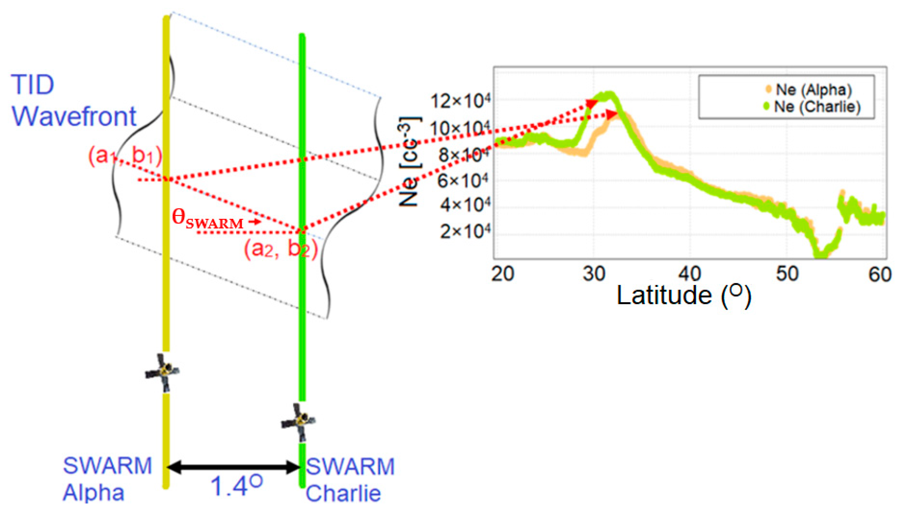
Despite being closely spaced, when Swarm A-C satellites encounter TID wavefronts at the same location recorded from the GPS d-TEC map, a clear TID propagation azimuth can be inferred from similar horizontal electron density fluctuations. This is measured by both Swarm A and Swarm C satellites, as shown in
Figure 1, which demonstrates the scenario of the Swarm A-C pair flying through a TID wavefront. The azimuth of the TID propagation (θ
SWARM) can be calculated between crests or troughs of horizontal electron density perturbations for both Swarm A and C when they encounter TID wavefronts. The propagation azimuth can be calculated by
where (a
1, b
1) are the coordinates of the point of intersection for Swarm A and the TID wavefront, and (a
2, b
2) are the coordinates of the point of intersection for Swarm C. For the small distances covered by the satellites within the limited time interval under consideration, we can make a simplification and use the difference of latitudes (degree intervals) instead of the difference of distances (range intervals). In fact, if the TID is appearing at high latitudes, we need to apply a correction factor to account for this. For the estimation of θ
GPS, a similar approach with the estimation of θ
SWARM was undertaken, but slightly differently to account for the fact that the actual points on the GPS d-TEC map used for the estimation of θ
GPS are more distant than the corresponding points for the estimation of θ
SWARM, which by default are separated by 1.4° in longitude (and are therefore quite close).
where
4. Validation
4.1. Japan TID Events
To validate our approach, we exploited the high density of GNSS stations in the Japanese longitude sector (latitude range: 24° to 48°N and longitude range: 124° to 148°E) to identify the signature of TID wavefronts during the summer of 2020 from the corresponding GPS d-TEC maps. The dense GNSS network provides the ideal scenario for such a validation purpose since the TID wavefronts can be identified on the d-TEC map. This was demonstrated, for example, by Otsuka et al. (2011) [
13], who detected most TID cases in Japan during a summer season. Kil and Paxton (2017) [
20] have adopted a similar approach, as demonstrated in [
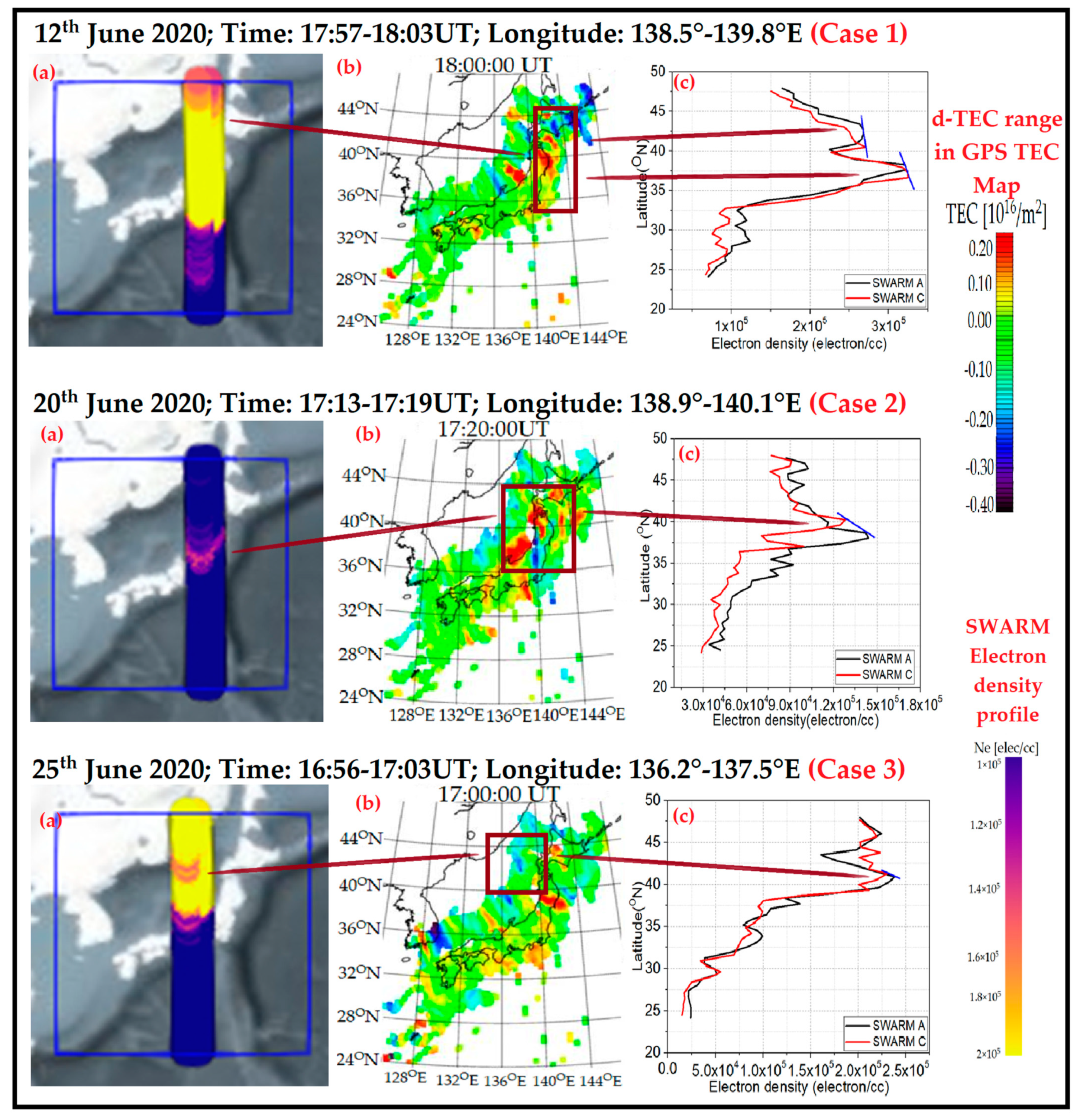
13], to examine TID occurrence from Swarm electron density measurements and thereby validate the presence of TIDs from d-TEC maps over Japan from 2013 to 2017. Twenty-seven TID cases have been detected over Japan during this period with the GPS d-TEC perturbation collocated with Swarm A-C electron density fluctuations. Among those cases, three TID wavefront cases are shown in
Figure 2.
A. Case 1 was registered from 17:57 to 18:03 UT on 12 June 2020 over the longitude range of 138.5° to 139.8°E. In the Case 1 diagram,
Figure 2a shows the location of Swarm A-C pass over Japan,
Figure 2b the GPS d-TEC map over Japan around the same time interval (the rectangle represents the position of the TID wavefront considered for this case) and
Figure 2c represents the horizontal electron density profile of Swarm A-C, where the black line stands for Swarm A and the red for Swarm C. Two peaks in the horizontal electron density profile of Swarm A-C were noted during 17:59:28 UT and 18:00:36 UT. The TID wavefront propagation azimuth θ
SWARM was estimated around 17:59:28UT at 23.5° and around 18:00:36 UT at 10.5° (
Figure 2c). The corresponding azimuth values θ
GPS for the GPS d-TEC perturbation were 22.5° and 11.9°, respectively.
B. Case 2 was recorded on 20 June 2020 from 17:13 to 17:19 UT over the longitude swath of 138.9° to 140.1°E. One peak in the horizontal electron density profile of Swarm A-C was observed during 17:15:29 UT with θSWARM of 62.4° and θGPS of 62.1°.
C. On 25 June 2020,
Case 3 was noted from 16:56 to 17:03 UT over the longitude sector of 136.2° to 137.5°E. In this case, a single horizontal electron density profile peak of Swarm A-C was also observed at 16:59:03 UT in
Figure 2c, with θ
SWARM of 68.2° and θ
GPS of 68.1°.
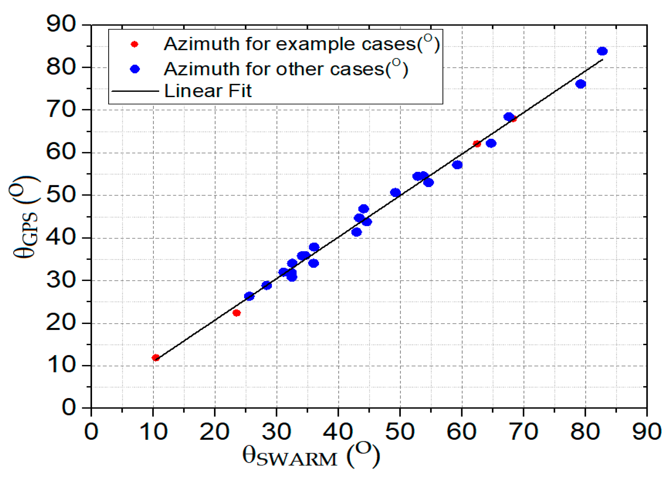
Figure 3 presents the scatter plot of θ
SWARM versus θ
GPS for Japan during June 2020. The red dots indicate the adopted cases mentioned above whereas the blue dots stand for all other TID cases detected over Japan in June 2020. The Figure demonstrates a high correlation with a r
2 (regression value) of around 0.992.
4.2. Europe TID Events
Over the European longitude sector (latitude range: 34° to 70°N and longitude range: −10° to 40°E), we used GPS d-TEC maps to identify TID events from 2015 to 2017. Otsuka et al. (2013) [
3] have studied TIDs in Europe and concluded that the occurrence of nighttime TIDs maximizes in winter. Paul et al. (2021) [
25] have presented a statistical study on the occurrence of satellite traces (ST) and multiple reflected echoes (MRE), which are ionogram TID signatures [
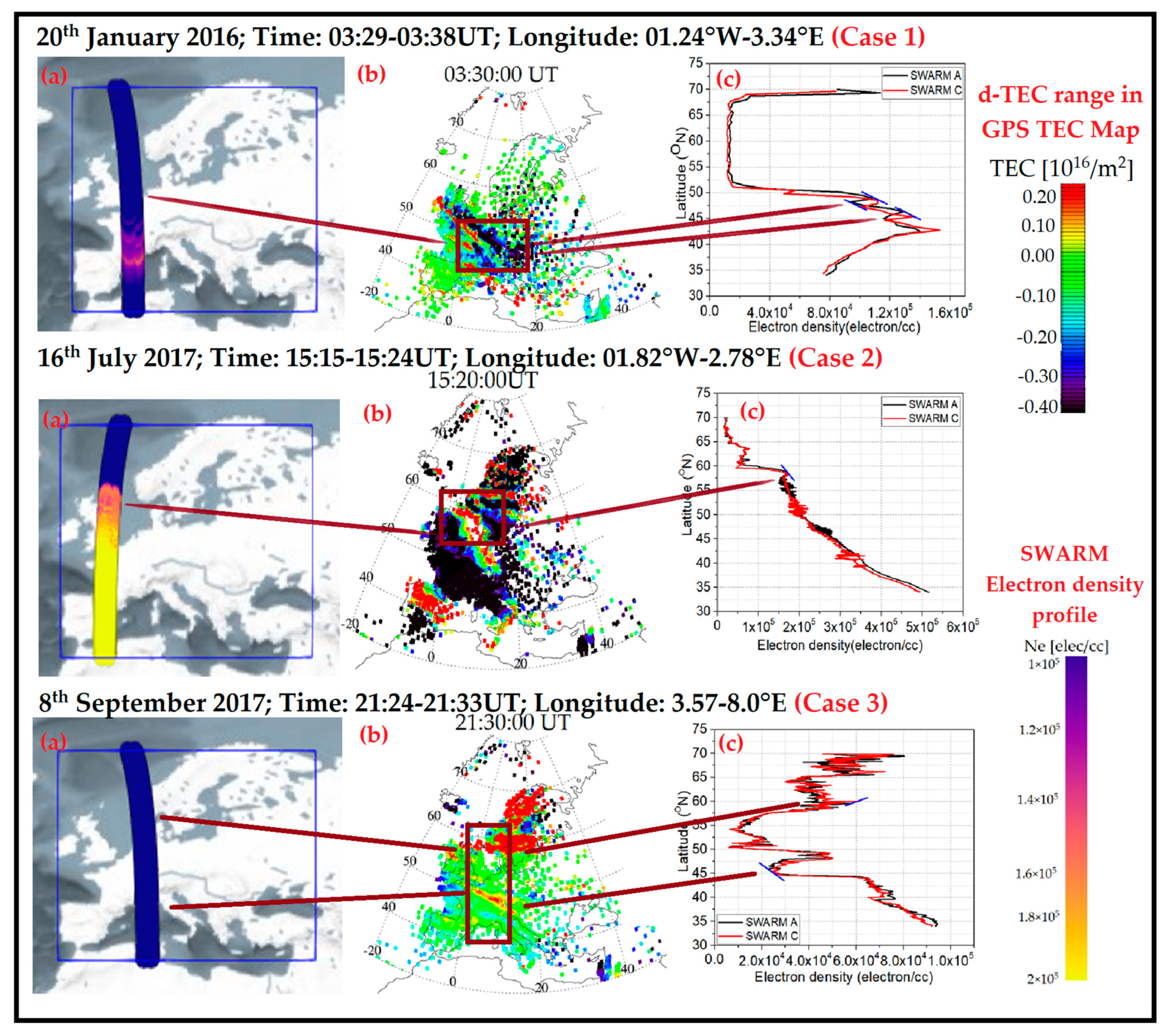
16], over Cyprus (low-latitude European station) and reported a maximum occurrence of these signatures during summer and equinoctial periods. In the present study, we focus on TID signatures over Europe from 2015 to 2017 for which Swarm passes coincide with available d-TEC maps. During this period, 16 cases with GPS d-TEC perturbation that collocated with Swarm A-C horizontal electron density fluctuations were identified, and among those, three are presented as example cases in
Figure 4.
A. Case 1 was recorded on 20 January 2016 from 03:29 to 03:38 UT over −01.24° to 03.34°E longitude range. Two peaks in the horizontal electron density profile of Swarm A-C were noted during 03:35:17 UT and 03:36:04 UT. The TID propagation azimuth (θ
SWARM) was 37.04° and 32.35°, around 03:35:17 UT and 03:36:04 UT, respectively (
Figure 4c). The corresponding azimuth θ
GPS for these cases was 37.89° and 36.65°, respectively.
B. On 16 July 2017, Case 2 was identified from 15:15 to 15:24 UT over −01.82° to 02.78°E longitude zone. A single peak in the horizontal electron density profile of Swarm A-C was recorded at 15:21:00 UT, with 42.21° for θSWARM and 42.71° for θGPS.
C. Case 3 was recorded on 8 September 2017 from 21:24 to 21:33 UT over the 03.57° to 08.00°E longitude range. Two horizontal electron density profile peaks of Swarm A-C was observed at 21:26:00 UT and 21:30:00 UT in
Figure 4c, with θ
SWARM estimated at 70.46° and 55.56°, where θ
GPS was 70.01° and 55.55°, respectively.
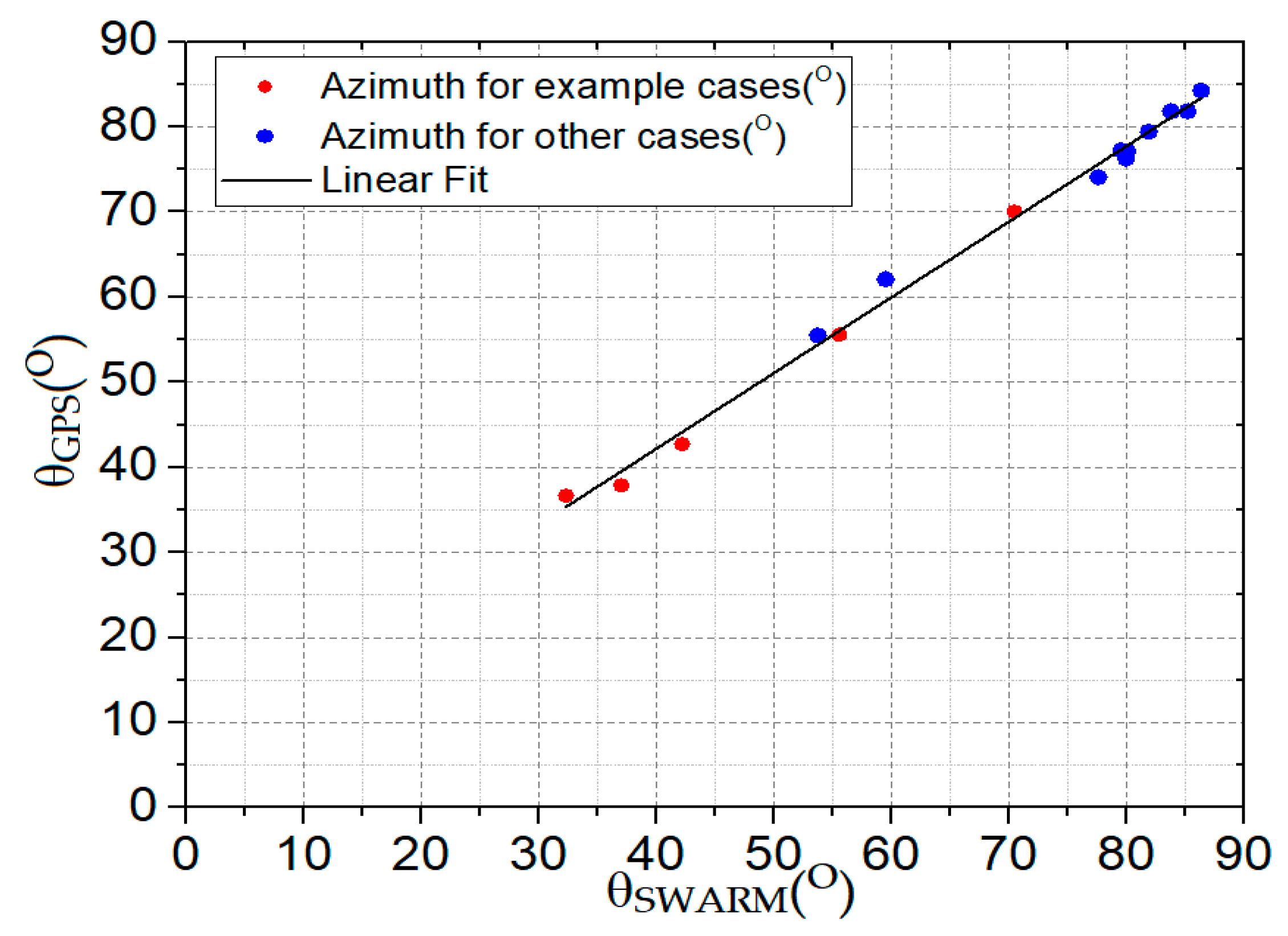
To investigate the correlation between θ
SWARM and θ
GPS, we have recorded 16 cases over Europe from 2015 to 2017. The scatter plot between θ
SWARM and θ
GPS, presented in
Figure 5, corresponds to a high correlation coefficient between θ
SWARM and θ
GPS with a r
2 (regression value) of around 0.994. In the plot, red dots represent the azimuth for the case studies used in the previous section whereas the blue dots stand for the other cases considered over Europe from 2015 to 2017.
4.3. North America TID Events
TID cases from GPS d-TEC maps over North American longitude (latitude range: 20° to 60°N and longitude range: −130° to −60°E) from 2015 to 2017 were also used to extend our validation over a wide geographical scope. Thirty-one TID cases were detected from GPS d-TEC maps for which Swarm A-C horizontal electron density profiles also captured the corresponding TID wavefronts.
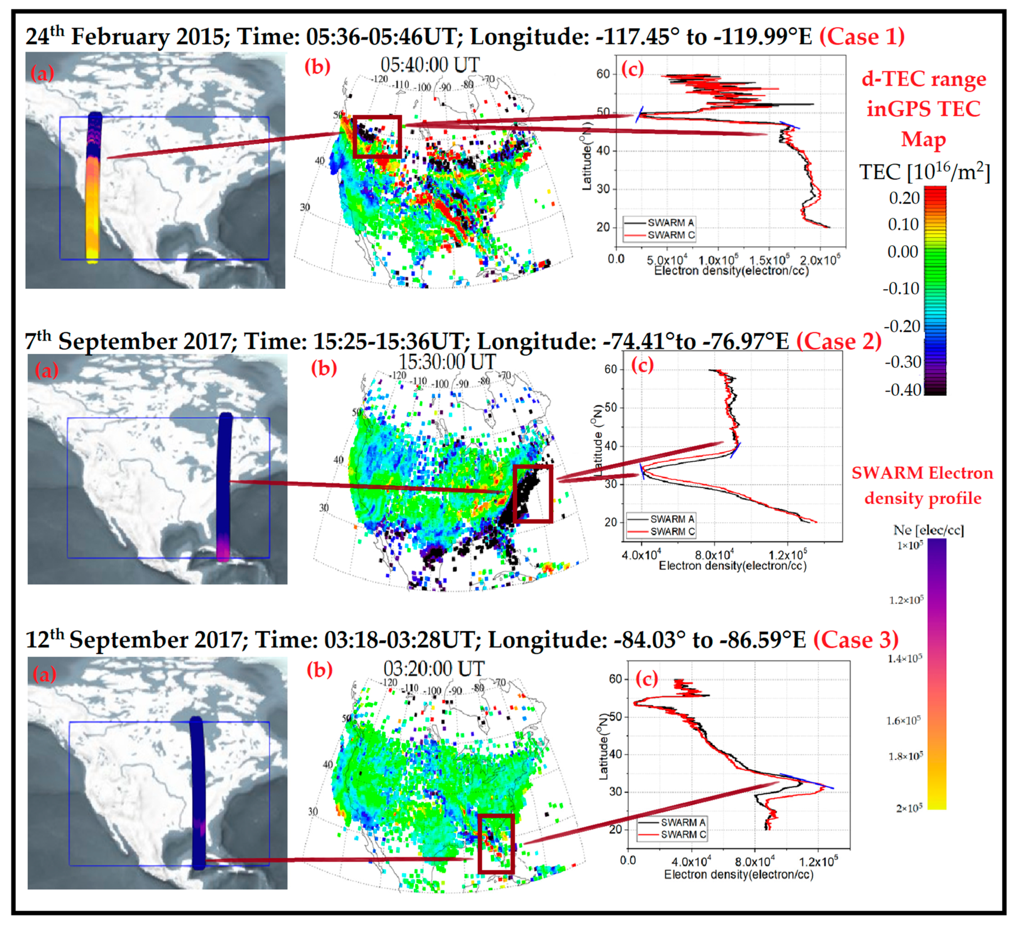
Figure 6 presents three cases in North America.
A. Case 1 was registered on 24 February 2015 from 05:36 to 05:46 UT over the longitude range of −117.45° to −119.99°E. Two peaks in the horizontal electron density profile of Swarm A-C were noted during 05:43:07 UT and 05:43:53 UT. The azimuth of TID propagation (θ
SWARM) recorded in the horizontal electron density profile peak was 70.46° and 24.62° around 05:43:07 UT and 05:43:53 UT, respectively (
Figure 6c). The corresponding azimuth θ
GPS estimated from GPS d-TEC maps were 70.35° and 24.98°.
B. On 7 September 2017, Case 2 was detected from 15:25 to 15:36 UT over the −74.41° to −76.97°E longitude range. Two horizontal electron density peaks of Swarm A-C were recorded at 15:29:19 UT and 15:30:35 UT, with θSWARM at 13.76° and 35.31° and θGPS at 13.59° and 35.02°, respectively.
C. Case 3 was registered on 12 September 2017 from 03:18 to 03:28 UT over the −84.03° to −86.59°E longitude range. A single horizontal electron density profile peak from Swarm A-C was detected at 03:25:31 UT in
Figure 6c, with θ
SWARM at 75:06° and θ
GPS at 75.37°.
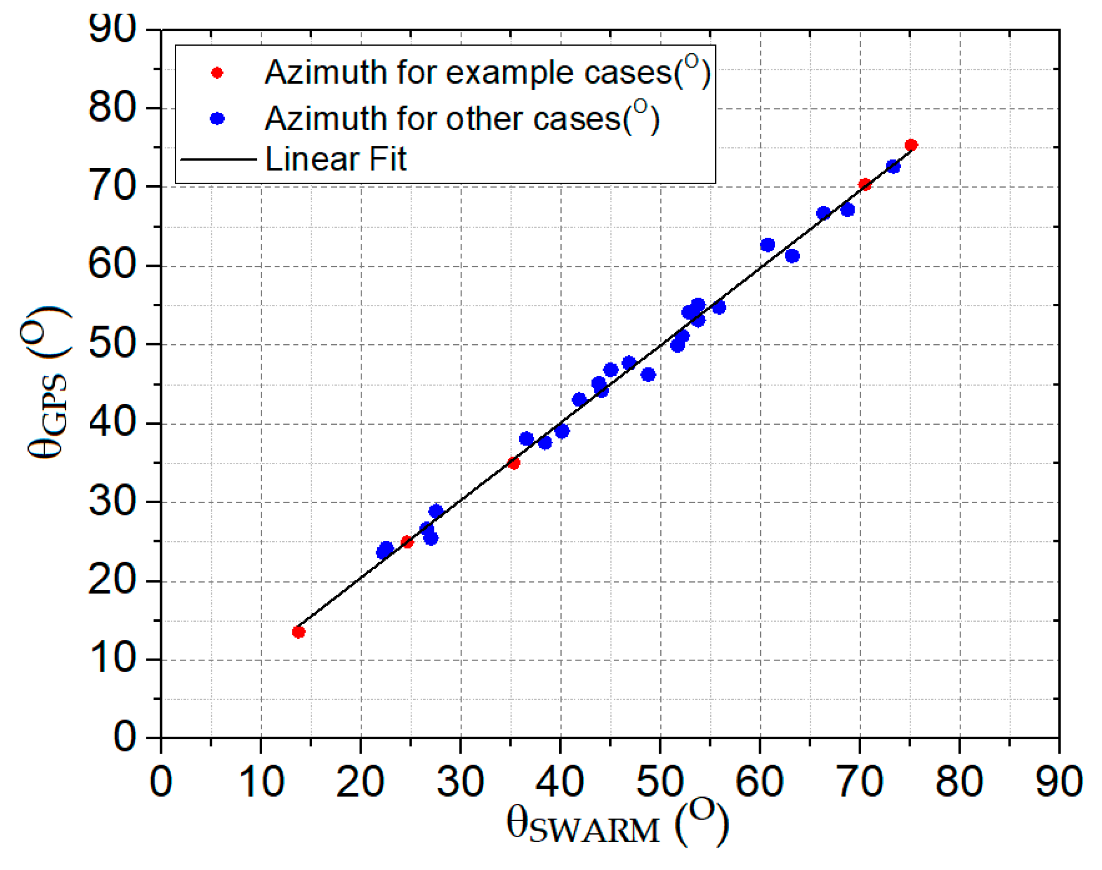
Figure 7 depicts the correlation between θ
SWARM and θ
GPS for 31 cases observed over North America from 2015 to 2017. The red dots represent the azimuth for the example cases presented above whereas the blue dots indicate the remaining cases
. The correlation coefficient is quite high with a r
2 (regression value) around 0.994.
For all the cases that were considered in the validation of the proposed TID direction detection technique, the latitude range covered by Swarm satellites in each case was carefully matched to the corresponding latitude range in the d-TEC map. That was also the case for the corresponding time intervals for these ranges. For all cases examined, we were able to detect the same number of crests or troughs in both Swarm data and d-TEC maps, which supported our approach. This study focuses on the validation of our simple method and not on its application to detect TID events in an operational context, which can be a challenging task considering the short-term electron density fluctuations (with much shorter amplitude than those caused by MSTIDs) superimposed on the horizontal electron density profiles, as measured by Swarm satellites. However, a more refined version with appropriate pre-processing of data to remove short-term electron density fluctuations could be suitable in order to collect statistics of the direction of propagation of TID wavefronts over the ocean and polar regions where ground-based GNSS stations are unavailable.


