
Boost Correlation Features with 3D-MiIoU-Based Camera-LiDAR Fusion for MODT in Autonomous Driving

Abstract
:1. Introduction
- This paper presents an end-to-end network named boost correlation multi-object detection tracking (BcMODT). BcMODT can simultaneously generate 3D bounding boxes and more accurate association scores from camera and LiDAR measurement data for real-time detection by using the boost correlation feature (BcF);
- This paper proposes a new 3D-CIoU computing module, enhancing the fault tolerance of intersection-over-union (IoU) computing. This 3D-CIoU can handle more scenarios by using the length-to-width and length-to-height ratios of the detected bounding box and tracked bounding box;
- We combine 3D-GIoU and 3D-CIoU, named 3D mixed IoU (3D-MiIoU), instead of 3D mean IoU (3D-Mean-IoU) in [8], as the calculation method for geometric affinity, which can express the geometric affinity between objects more carefully;
- The approach is evaluated on the large autonomous driving benchmark KITTI [9], and the results show that compared with existing methods, the proposed method effectively improves the tracking accuracy, IDSW, and other evaluation metrics.
2. Related Works
2.1. Multi-Object Tracking Framework
2.2. Affinity Metrics for Object Detection
2.2.1. Appearance Modality
2.2.2. Motion and Geometry
3. Methodology
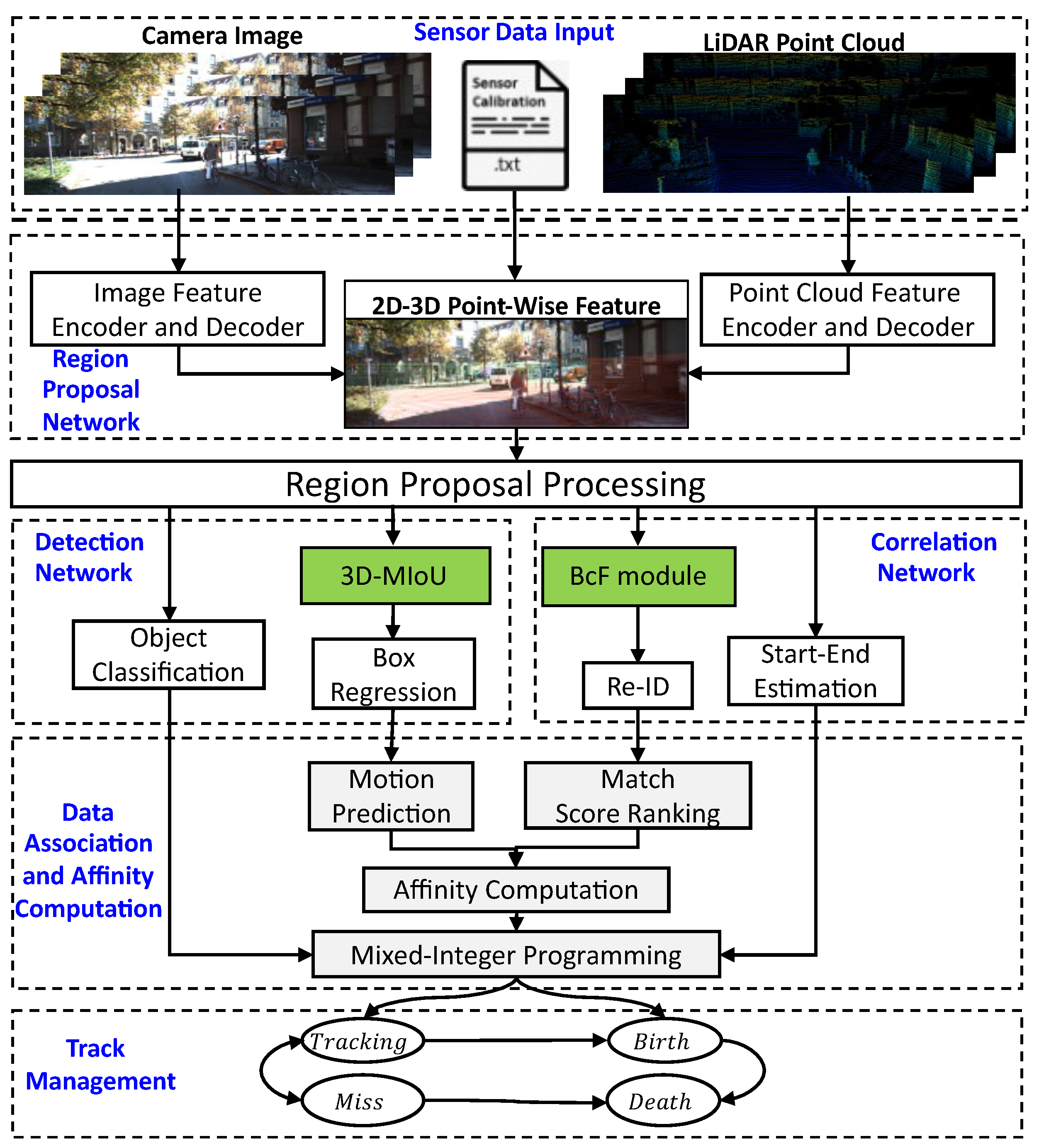
3.1. System Architecture
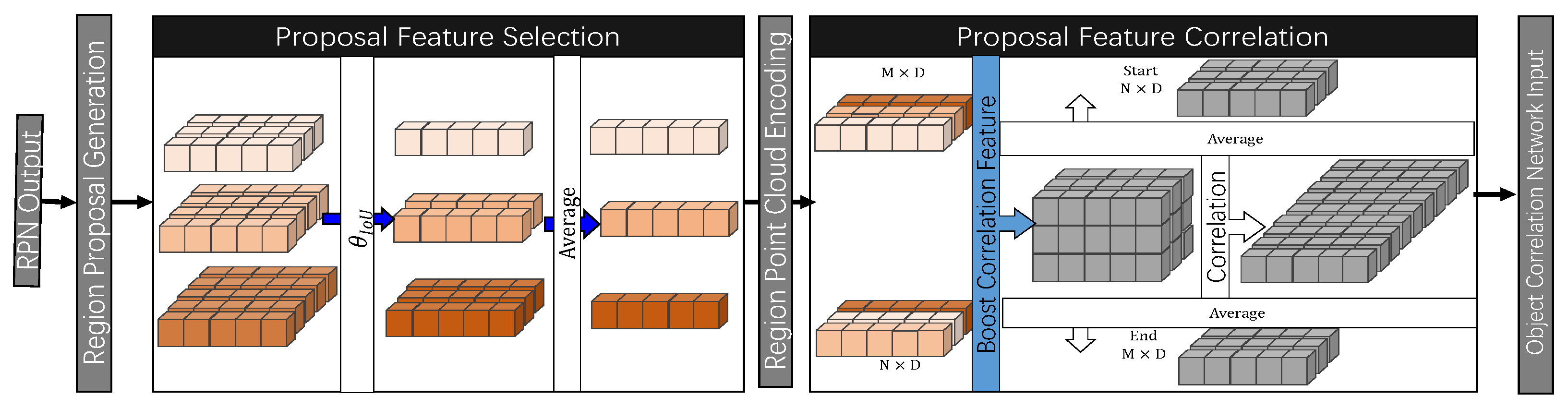
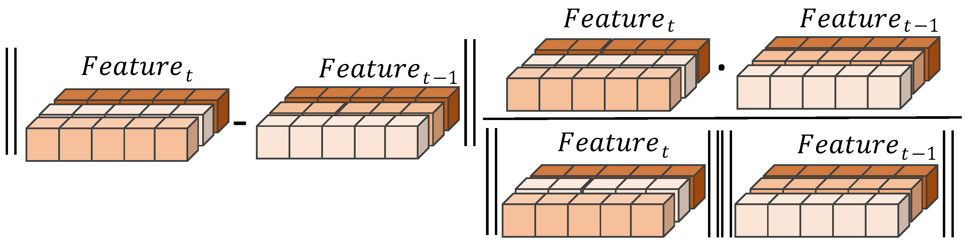
3.2. Boost Correlation Feature
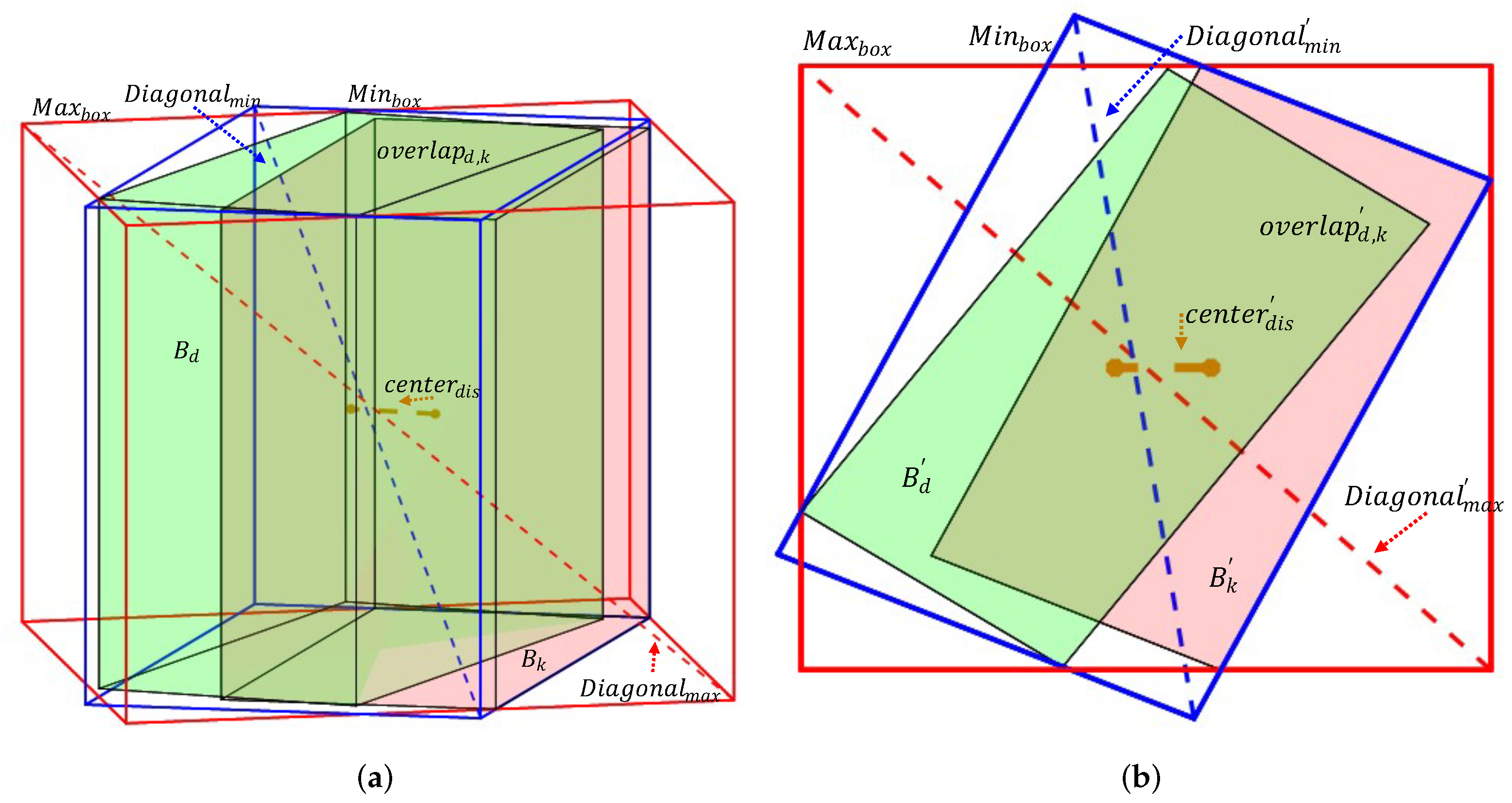
3.3. 3D-IoU
3.3.1. 3D-GIoU
3.3.2. 3D-CIoU
3.3.3. 3D-MiIoU
| Algorithm 1 Three-dimensional mixed intersection over union. |
|
3.4. Affinity Computation
| Algorithm 2 Affinity metric with BcF and 3D-MiIoU. |
|
3.5. Time Complexity
4. Experiments
4.1. Experimental Settings
4.2. Baseline and Evaluation Metrics
4.3. Quantitative Results
4.4. Ablation Experiments
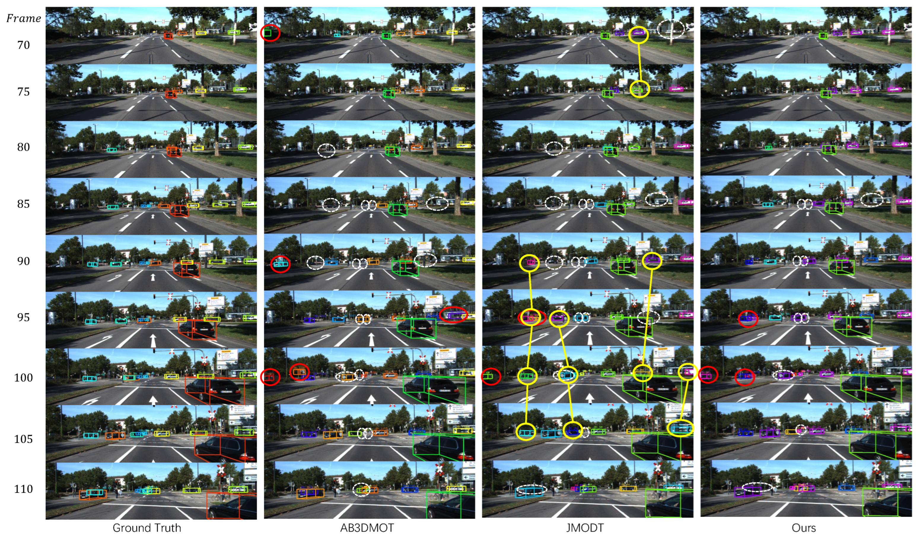
4.5. Qualitative Results
4.6. Limitations
5. Conclusions
Author Contributions
Funding
Informed Consent Statement
Data Availability Statement
Conflicts of Interest
References
- Weng, X.; Wang, Y.; Man, Y.; Kitani, K.M. Gnn3dmot: Graph neural network for 3d multi-object tracking with 2d-3d multi-feature learning. In Proceedings of the IEEE/CVF Conference on Computer Vision and Pattern Recognition, Seattle, WA, USA, 13–19 June 2020; pp. 6499–6508. [Google Scholar]
- Wu, J.; Cao, J.; Song, L.; Wang, Y.; Yang, M.; Yuan, J. Track to detect and segment: An online multi-object tracker. In Proceedings of the IEEE/CVF Conference on Computer Vision and Pattern Recognition, Nashville, TN, USA, 20–25 June 2021; pp. 12352–12361. [Google Scholar]
- Leibe, B.; Schindler, K.; Van Gool, L. Coupled detection and trajectory estimation for multi-object tracking. In Proceedings of the 2007 IEEE 11th International Conference on Computer Vision, Rio de Janeiro, Brazil, 14–21 October 2007; pp. 1–8. [Google Scholar]
- Feng, D.; Haase-Schütz, C.; Rosenbaum, L.; Hertlein, H.; Glaeser, C.; Timm, F.; Wiesbeck, W.; Dietmayer, K. Deep multi-modal object detection and semantic segmentation for autonomous driving: Datasets, methods, and challenges. IEEE Trans. Intell. Transp. Syst. 2020, 22, 1341–1360. [Google Scholar] [CrossRef]
- Kim, A.; Ošep, A.; Leal-Taixé, L. Eagermot: 3d multi-object tracking via sensor fusion. In Proceedings of the 2021 IEEE International Conference on Robotics and Automation (ICRA), Xi’an, China, 30 May–5 June 2021; pp. 11315–11321. [Google Scholar]
- Shenoi, A.; Patel, M.; Gwak, J.; Goebel, P.; Sadeghian, A.; Rezatofighi, H.; Martin-Martin, R.; Savarese, S. Jrmot: A real-time 3d multi-object tracker and a new large-scale dataset. In Proceedings of the 2020 IEEE/RSJ International Conference on Intelligent Robots and Systems (IROS), Las Vegas, NV, USA, 25–29 October 2020; pp. 10335–10342. [Google Scholar]
- Zhang, W.; Zhou, H.; Sun, S.; Wang, Z.; Shi, J.; Loy, C.C. Robust multi-modality multi-object tracking. In Proceedings of the IEEE/CVF International Conference on Computer Vision, Seoul, Republic of Korea, 27–28 October 2019; pp. 2365–2374. [Google Scholar]
- Gonzalez, N.F.; Ospina, A.; Calvez, P. Smat: Smart multiple affinity metrics for multiple object tracking. In Proceedings of the International Conference on Image Analysis and Recognition, Povoa de Varzim, Portugal, 24–26 June 2020; pp. 48–62. [Google Scholar]
- Geiger, A.; Lenz, P.; Urtasun, R. Are we ready for Autonomous Driving? The KITTI Vision Benchmark Suite. In Proceedings of the Conference on Computer Vision and Pattern Recognition (CVPR), Providence, RI, USA, 16–21 June 2012. [Google Scholar]
- Li, Y.; Huang, C.; Nevatia, R. Learning to associate: Hybridboosted multi-target tracker for crowded scene. In Proceedings of the 2009 IEEE Conference on Computer Vision and Pattern Recognition, Miami, FL, USA, 20–25 June 2009; pp. 2953–2960. [Google Scholar]
- Weng, X.; Wang, J.; Held, D.; Kitani, K. Ab3dmot: A baseline for 3d multi-object tracking and new evaluation metrics. arXiv 2020, arXiv:2008.08063. [Google Scholar]
- An, J.; Zhang, D.; Xu, K.; Wang, D. An OpenCL-Based FPGA Accelerator for Faster R-CNN. Entropy 2022, 24, 1346. [Google Scholar] [CrossRef]
- Lu, Z.; Rathod, V.; Votel, R.; Huang, J. Retinatrack: Online single stage joint detection and tracking. In Proceedings of the IEEE/CVF Conference on Computer Vision and Pattern Recognition, Seattle, WA, USA, 13–19 June 2020; pp. 14668–14678. [Google Scholar]
- Zhou, X.; Koltun, V.; Krähenbühl, P. Tracking objects as points. In Proceedings of the European Conference on Computer Vision, Glasgow, UK, 23–28 August 2020; pp. 474–490. [Google Scholar]
- Peng, J.; Wang, C.; Wan, F.; Wu, Y.; Wang, Y.; Tai, Y.; Wang, C.; Li, J.; Huang, F.; Fu, Y. Chained-tracker: Chaining paired attentive regression results for end-to-end joint multiple-object detection and tracking. In Proceedings of the European Conference on Computer Vision, Glasgow, UK, 23–28 August 2020; pp. 145–161. [Google Scholar]
- Wang, Z.; Zheng, L.; Liu, Y.; Li, Y.; Wang, S. Towards real-time multi-object tracking. In Proceedings of the European Conference on Computer Vision, Glasgow, UK, 23–28 August 2020; pp. 107–122. [Google Scholar]
- Huang, K.; Hao, Q. Joint Multi-Object Detection and Tracking with Camera-LiDAR Fusion for Autonomous Driving. In Proceedings of the 2021 IEEE/RSJ International Conference on Intelligent Robots and Systems (IROS), Prague, Czech Republic, 27 September–1 October 2021; pp. 6983–6989. [Google Scholar]
- Qi, C.R.; Liu, W.; Wu, C.; Su, H.; Guibas, L.J. Frustum pointnets for 3d object detection from rgb-d data. In Proceedings of the IEEE Conference on Computer Vision and Pattern Recognition, Salt Lake, UT, USA, 18–23 June 2018; pp. 918–927. [Google Scholar]
- Mykheievskyi, D.; Borysenko, D.; Porokhonskyy, V. Learning local feature descriptors for multiple object tracking. In Proceedings of the Asian Conference on Computer Vision, Kyoto, Japan, 30 November–4 December 2020. [Google Scholar]
- Wu, Y.; Liu, Z.; Chen, Y.; Zheng, X.; Zhang, Q.; Yang, M.; Tang, G. FCNet: Stereo 3D Object Detection with Feature Correlation Networks. Entropy 2022, 24, 1121. [Google Scholar] [CrossRef] [PubMed]
- Zhao, M.; Jha, A.; Liu, Q.; Millis, B.A.; Mahadevan-Jansen, A.; Lu, L.; Landman, B.A.; Tyska, M.J.; Huo, Y. Faster Mean-shift: GPU-accelerated clustering for cosine embedding-based cell segmentation and tracking. Med. Image Anal. 2021, 71, 102048. [Google Scholar] [CrossRef] [PubMed]
- You, L.; Jiang, H.; Hu, J.; Chang, C.H.; Chen, L.; Cui, X.; Zhao, M. GPU-accelerated Faster Mean Shift with euclidean distance metrics. In Proceedings of the 2022 IEEE 46th Annual Computers, Software, and Applications Conference (COMPSAC), Los Alamitos, CA, USA, 27 June–1 July 2022; pp. 211–216. [Google Scholar]
- Jiang, B.; Luo, R.; Mao, J.; Xiao, T.; Jiang, Y. Acquisition of localization confidence for accurate object detection. In Proceedings of the European conference on computer vision (ECCV), Munich, Germany, 8–14 September 2018; pp. 784–799. [Google Scholar]
- Yu, J.; Jiang, Y.; Wang, Z.; Cao, Z.; Huang, T. Unitbox: An advanced object detection network. In Proceedings of the 24th ACM International Conference on Multimedia, Amsterdam, The Netherlands, 15–19 October 2016; pp. 516–520. [Google Scholar]
- Elhoseny, M. Multi-object detection and tracking (MODT) machine learning model for real-time video surveillance systems. Circuits Syst. Signal Process. 2020, 39, 611–630. [Google Scholar] [CrossRef]
- Farag, W. Kalman-filter-based sensor fusion applied to road-objects detection and tracking for autonomous vehicles. Proc. Inst. Mech. Eng. Part. J. Syst. Control Eng. 2021, 235, 1125–1138. [Google Scholar] [CrossRef]
- Bodla, N.; Singh, B.; Chellappa, R.; Davis, L.S. Soft-NMS–improving object detection with one line of code. In Proceedings of the IEEE International Conference on Computer Vision, Venice, Italy, 22–29 October 2017; pp. 5561–5569. [Google Scholar]
- Rezatofighi, H.; Tsoi, N.; Gwak, J.; Sadeghian, A.; Reid, I.; Savarese, S. Generalized intersection over union: A metric and a loss for bounding box regression. In Proceedings of the IEEE/CVF Conference on Computer Vision and Pattern Recognition, Long Beach, CA, USA, 15–20 June 2019; pp. 658–666. [Google Scholar]
- Zheng, Z.; Wang, P.; Liu, W.; Li, J.; Ye, R.; Ren, D. Distance-IoU Loss: Faster and Better Learning for Bounding Box Regression. arXiv 2019, arXiv:1911.08287. [Google Scholar] [CrossRef]
- Girshick, R.; Donahue, J.; Darrell, T.; Malik, J. Rich Feature Hierarchies for Accurate Object Detection and Semantic Segmentation. In Proceedings of the 2014 IEEE Conference on Computer Vision and Pattern Recognition, Columbus, OH, USA, 23–28 June 2014; pp. 580–587. [Google Scholar]
- Shi, S.; Wang, X.; Li, H. PointRCNN: 3D Object Proposal Generation and Detection From Point Cloud. In Proceedings of the 2019 IEEE/CVF Conference on Computer Vision and Pattern Recognition (CVPR), Long Beach, CA, USA, 15–20 June 2019; pp. 770–779. [Google Scholar]
- Nguyen, H.V.; Bai, L. Cosine similarity metric learning for face verification. In Proceedings of the Asian Conference on Computer Vision, Queenstown, New Zealand, 8–12 November 2010; pp. 709–720. [Google Scholar]
- Xu, J.; Ma, Y.; He, S.; Zhu, J. 3D-GIoU: 3D generalized intersection over union for object detection in point cloud. Sensors 2019, 19, 4093. [Google Scholar] [CrossRef] [PubMed]
- Chen, Y.; Li, H.; Gao, R.; Zhao, D. Boost 3-D object detection via point clouds segmentation and fused 3-D GIoU-L1 loss. IEEE Trans. Neural Netw. Learn. Syst. 2020, 33, 762–773. [Google Scholar] [CrossRef] [PubMed]
- Paszke, A.; Gross, S.; Chintala, S.; Chanan, G.; Yang, E.; DeVito, Z.; Lin, Z.; Desmaison, A.; Antiga, L.; Lerer, A. Automatic Differentiation in Pytorch. 2017. Available online: https://openreview.net/forum?id=BJJsrmfCZ (accessed on 20 November 2022).
- Huang, T.; Liu, Z.; Chen, X.; Bai, X. Epnet: Enhancing point features with image semantics for 3d object detection. In Proceedings of the European Conference on Computer Vision, Glasgow, UK, 23–28 August 2020; pp. 35–52. [Google Scholar]
- Loshchilov, I.; Hutter, F. Decoupled weight decay regularization. arXiv 2017, arXiv:1711.05101. [Google Scholar]
- Loshchilov, I.; Hutter, F. Sgdr: Stochastic gradient descent with warm restarts. arXiv 2016, arXiv:1608.03983. [Google Scholar]
- Bernardin, K.; Stiefelhagen, R. Evaluating multiple object tracking performance: The clear mot metrics. Eurasip. J. Image Video Process. 2008, 2008, 246309. [Google Scholar] [CrossRef] [Green Version]
- Luiten, J.; Osep, A.; Dendorfer, P.; Torr, P.; Geiger, A.; Leal-Taixé, L.; Leibe, B. Hota: A higher order metric for evaluating multi-object tracking. Int. J. Comput. Vis. 2021, 129, 548–578. [Google Scholar] [CrossRef] [PubMed]


| Type | Method | Object Detection and Correlation | Affinity Metrix | Data Asociation | Year | |||
|---|---|---|---|---|---|---|---|---|
| Detection | Correlation | Appearance Modality | Motion | Geometry | ||||
| TBD [10,11] | ODESA [19] | 2D | Re-ID | Camera | KF | 2D IoU | HA | 2020 |
| SMAT [8] | 2D | Re-ID Optical Flow | Camera | × | 2D IoU | HA | 2020 | |
| JRMOT [6] | 3D | Re-ID | Camera + LiDAR (Batch Fusion) | KF | 3D IoU | JPDA | 2020 | |
| mmMOT [7] | 3D | Re-ID Start-End | Camera + LiDAR | × | × | MIP | 2019 | |
| JDT [13,14,15,16,17] | CenterTrack [14] | 2D/3D | Paired Detection | Camera | Offset | 2D Distance | Greedy | 2020 |
| ChainedTrack [15] | 2D | Parallel Re-ID | Camera | × | 2D IoU | HA | 2020 | |
| JDE | 2D | Parallel Re-ID | Camera | KF | 2D Distance | HA | 2019 | |
| Retina Track [13] | 2D | Parallel Re-ID | Camera | KF | 2D IoU | HA | 2020 | |
| JMODT [17] | 3D | Parallel Re-ID Start-End | Camera + LiDAR (Point-Wise Fusion) | KF | 3D DIoU | Improved MIP | 2021 | |
| BcMODT (Ours) | 3D | Parallel Re-ID Start-End BcF | Camera + LiDAR (Point-Wise Fusion) BcF | KF | 3D MiIoU | Improved MIP | 2022 | |
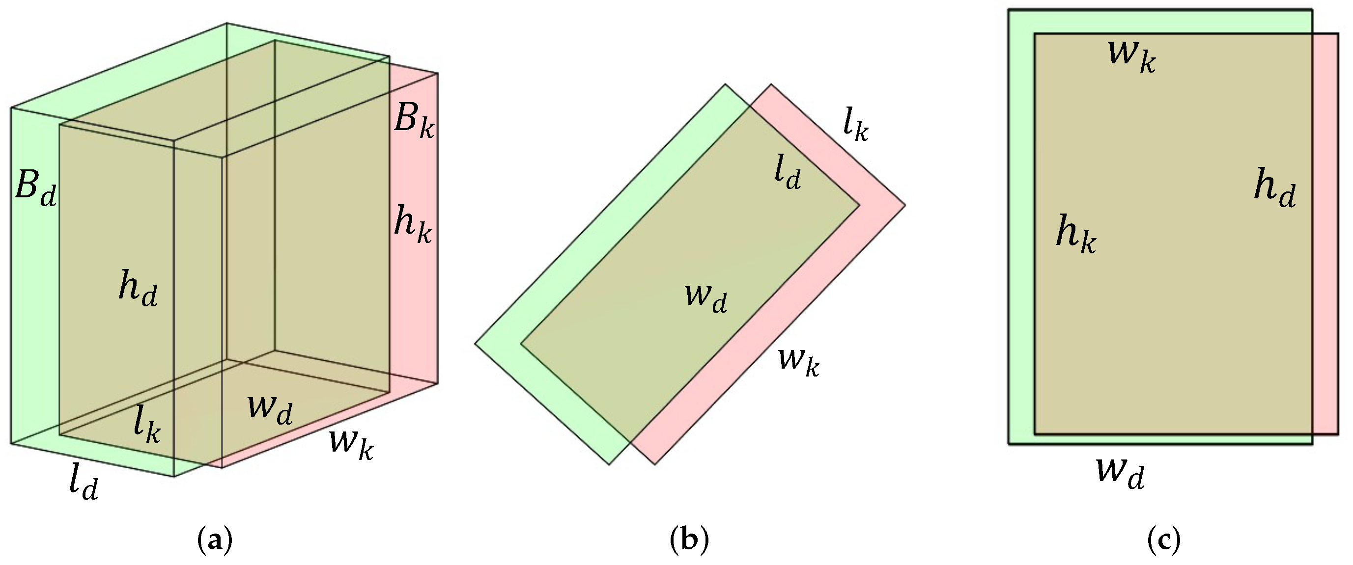
| Parameter | Description |
|---|---|
| Detected bounding box in 3D view. | |
| Tracked bounding box in 3D view. | |
| Detected bounding box in top view. | |
| Tracked bounding box in top view. | |
| The center distance of and in 3D view. | |
| The center distance of and in top view. | |
| Diagonal distance of . | |
| Diagonal distance of . | |
| in top view. | |
| in top view. | |
| Minimum bounding boxes of and . | |
| Maximum bounding boxes of and . | |
| The overlapping volume of and . | |
| Overlapping area of and . |
| Measure | Better | Perfect | Description |
|---|---|---|---|
| MOTA [39] | Higher | 100% | Multi-object tracking accuracy. |
| MOTP [39] | Higher | 100% | Multi-object tracking precision. |
| HOTA [40] | Higher | 100% | Higher-order tracking accuracy. |
| MT | Higher | 100% | Mostly tracked targets. |
| ML | Lower | 0% | Partly tracked targets. |
| FP | Lower | 0 | The total number of false positives. |
| FN | Lower | 0 | The total number of false negatives (missed targets). |
| IDSW | Lower | 0 | Number of identity switches. |
| FRAG | Lower | 0 | The total number of times a trajectory is fragmented. |
| Time | Lower | - | The total execution time. |
| FPS | Higher | - | Frames per second. |
| Method | AB3DMOT [11] | mmMOT [7] | JRMOT [6] | JMODT [17] | BcMOT Ours |
|---|---|---|---|---|---|
| Benchmark | Car | Car | Car | Car | Car |
| JDT | ✕ | ✕ | ✕ | ✔ | ✔ |
| AT | ✔ | ✔ | ✔ | ✕ | ✕ |
| MOTA↑ | 83.92% | 84.77% | 85.70% | 86.27% | 86.53% |
| MOTP↑ | 85.30% | 85.21% | 85.48% | 85.41% | 85.37% |
| MODA↑ | 83.95% | 85.60% | 85.98% | 86.40% | 86.66% |
| MODP↑ | 88.21% | 88.28% | 88.42% | 88.32% | 88.29% |
| TP↑ | 33,864 | 33,695 | 34,556 | 35,857 | 35,972 |
| FP↓ | 978 | 711 | 772 | 772 | 1248 |
| FN↓ | 4542 | 4243 | 4049 | 3433 | 3341 |
| MT↑ | 66.77% | 73.23% | 71.85% | 77.38% | 78.31% |
| ML↓ | 9.08% | 2.77% | 4.00% | 2.92% | 2.62% |
| IDSW↓ | 10 | 284 | 98 | 45 | 45 |
| Frag↓ | 199 | 753 | 372 | 585 | 626 |
| Runtime | 0.005 s | 0.002 s | 0.007 s | 0.001 s | 0.001 s |
| Method | AB3DMOT [11] | mmMOT [7] | JRMOT [6] | JMODT [17] | BcMOT Ours |
|---|---|---|---|---|---|
| Benchmark | Car | Car | Car | Car | Car |
| JDT | ✕ | ✕ | ✕ | ✔ | ✔ |
| AT | ✔ | ✔ | ✔ | ✕ | ✕ |
| HOTA↑ | 69.99% | 62.05% | 69.61% | 70.73% | 71.00% |
| MOTA↑ | 83.61% | 83.23% | 85.10% | 85.35% | 85.48% |
| MOTP↑ | 85.23% | 85.03% | 85.28% | 85.37% | 85.31% |
| TP↑ | 29,849 | 30,325 | 30,108 | 30,954 | 31,039 |
| FP↓ | 4543 | 4067 | 4284 | 3438 | 3353 |
| FN↓ | 979 | 787 | 752 | 1249 | 1260 |
| MT↑ | 66.92% | 72.92% | 70.92% | 77.39% | 78.15% |
| ML↓ | 9.08% | 2.92% | 4.62% | 2.92% | 2.62% |
| IDSW↓ | 113 | 733 | 271 | 350 | 381 |
| Frag↓ | 206 | 570 | 273 | 693 | 732 |
| Runtime | 0.005 s | 0.002 s | 0.007 s | 0.001 s | 0.001 s |
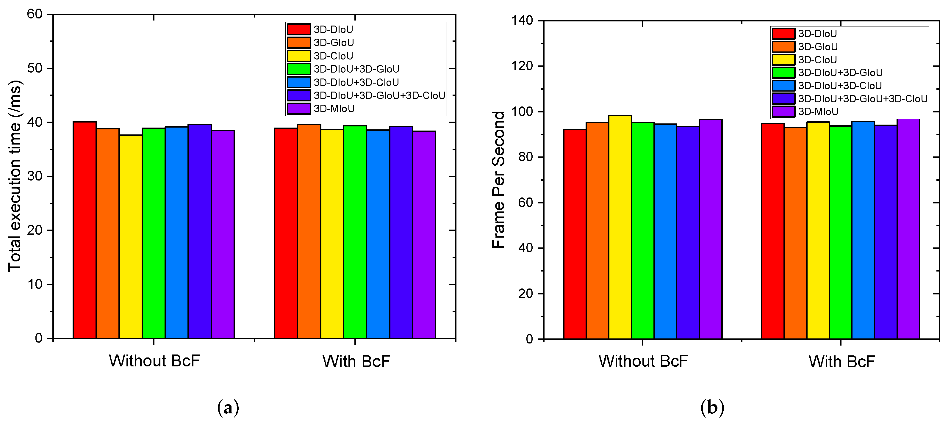
| Measure | BcF | MOTA↑ | MOTP↑ | MT↑ | ML↓ | FP↓ | FN↓ | IDSW↓ | Frag↓ | Time↓ | FPS↑ |
|---|---|---|---|---|---|---|---|---|---|---|---|
| 3D-DIoU | ✕ | 86.09% | 87.13% | 86.11% | 1.39% | 545 | 997 | 4 | 144 | 40.11 | 92.24 |
| ✔ | 86.36% | 87.16% | 85.65% | 1.39% | 531 | 984 | 1 | 137 | 38.901 | 94.83 | |
| 3D-GIoU | ✕ | 86.15% | 87.15% | 86.11% | 1.39% | 531 | 1004 | 4 | 144 | 38.84 | 95.27 |
| ✔ | 86.39% | 87.17% | 85.19% | 1.39% | 516 | 993 | 5 | 139 | 39.629 | 95.11 | |
| 3D-CIoU | ✕ | 85.82% | 87.25% | 84.72% | 1.85% | 500 | 1072 | 4 | 144 | 37.63 | 98.32 |
| ✔ | 86.11% | 87.26% | 85.19% | 1.85% | 486 | 1055 | 3 | 137 | 38.69 | 95.36 | |
| 3D-DIoU 3D-GIoU | ✕ | 86.12 % | 87.10% | 86.11% | 1.39% | 564 | 977 | 2 | 141 | 38.87 | 95.20 |
| ✔ | 86.42% | 87.12% | 85.65% | 1.39% | 546 | 962 | 1 | 137 | 39.35 | 93.75 | |
| 3D-DIoU 3D-CIoU | ✕ | 86.06 % | 87.13% | 86.11% | 1.39% | 546 | 999 | 4 | 144 | 39.14 | 94.53 |
| ✔ | 86.39% | 87.16% | 85.65% | 1.39% | 526 | 987 | 0 | 137 | 38.57 | 95.71 | |
| 3D-DIoU 3D-GIoU 3D-CIoU | ✕ | 86.10% | 87.10% | 86.11% | 1.39% | 565 | 978 | 2 | 141 | 39.59 | 93.45 |
| ✔ | 86.46% | 87.12% | 85.65% | 1.39% | 541 | 964 | 0 | 137 | 39.26 | 93.96 | |
| 3D-MiIoU (Ours) | ✕ | 86.29% | 87.19% | 85.65% | 1.39% | 527 | 993 | 4 | 127 | 38.50 | 96.69 |
| ✔ | 86.66% | 87.18% | 86.57% | 1.39% | 490 | 990 | 3 | 142 | 38.34 | 97.29 |
Disclaimer/Publisher’s Note: The statements, opinions and data contained in all publications are solely those of the individual author(s) and contributor(s) and not of MDPI and/or the editor(s). MDPI and/or the editor(s) disclaim responsibility for any injury to people or property resulting from any ideas, methods, instructions or products referred to in the content. |
© 2023 by the authors. Licensee MDPI, Basel, Switzerland. This article is an open access article distributed under the terms and conditions of the Creative Commons Attribution (CC BY) license (https://creativecommons.org/licenses/by/4.0/).
Share and Cite
Zhang, K.; Liu, Y.; Mei, F.; Jin, J.; Wang, Y. Boost Correlation Features with 3D-MiIoU-Based Camera-LiDAR Fusion for MODT in Autonomous Driving. Remote Sens. 2023, 15, 874. https://doi.org/10.3390/rs15040874
Zhang K, Liu Y, Mei F, Jin J, Wang Y. Boost Correlation Features with 3D-MiIoU-Based Camera-LiDAR Fusion for MODT in Autonomous Driving. Remote Sensing. 2023; 15(4):874. https://doi.org/10.3390/rs15040874
Chicago/Turabian StyleZhang, Kunpeng, Yanheng Liu, Fang Mei, Jingyi Jin, and Yiming Wang. 2023. "Boost Correlation Features with 3D-MiIoU-Based Camera-LiDAR Fusion for MODT in Autonomous Driving" Remote Sensing 15, no. 4: 874. https://doi.org/10.3390/rs15040874