Graph-Based Domain Adaptation Few-Shot Learning for Hyperspectral Image Classification

Abstract

Due to a lack of labeled samples, deep learning methods generally tend to have poor classification performance in practical applications. Few-shot learning (FSL), as an emerging learning paradigm, has been widely utilized in hyperspectral image (HSI) classification with limited labeled samples. However, the existing FSL methods generally ignore the domain shift problem in cross-domain scenes and rarely explore the associations between samples in the source and target domain. To tackle the above issues, a graph-based domain adaptation FSL (GDAFSL) method is proposed for HSI classification with limited training samples, which utilizes the graph method to guide the domain adaptation learning process in a uniformed framework. First, a novel deep residual hybrid attention network (DRHAN) is designed to extract discriminative embedded features efficiently for few-shot HSI classification. Then, a graph-based domain adaptation network (GDAN), which combines graph construction with domain adversarial strategy, is proposed to fully explore the domain correlation between source and target embedded features. By utilizing the fully explored domain correlations to guide the domain adaptation process, a domain invariant feature metric space is learned for few-shot HSI classification. Comprehensive experimental results conducted on three public HSI datasets demonstrate that GDAFSL is superior to the state-of-the-art with a small sample size.

1. Introduction

Hyperspectral images (HSIs) generally consist of a series of continuous spectral bands and contain abundant spectral characteristic information. By utilizing such abundant HSI information, ground objects can be identified and classified into a specific category accurately. As the cornerstone of HSI applications, HSI classification has been widely implemented in various practical applications, such as urban development [1], environmental protection [2], precision agriculture [3], and geological exploration [4].

As a powerful feature extraction method, deep learning has been widely utilized to classify HSI and achieved satisfactory classification results. Firstly, the stacked autoencoder (SAE) [5] and deep belief network (DBN) [6] were developed to perform HSI classification. However, the above-mentioned methods generally take 1-D pixel vectors as the inputs of deep models, which ignores the complex context information in 3-D pixel neighborhoods. In addition, a large amount of parameters requires to be optimized because of the models constructed by fully connected layers (FC). To address these issues, some works [7,8,9,10] introduced a convolutional neural network (CNN) to learn deep feature representation, which directly processes 3-D pixel neighborhoods without discarding context information. For example, a regularized deep feature extraction (FE) method [7] is designed to extract discriminative features by utilizing a CNN consisting of several convolutional and pooling layers. Subsequently, in order to fully utilize spectral-spatial information in HSI pixel neighborhoods, some works [11,12,13] introduced 3-D CNNs to synchronously learn spectral and spatial deep features for HSI classification. Li et al. [11] designed a spectral-spatial deep model constructed by 3-D CNNs to jointly learn deep semantic features for HSI classification.

However, as the network deepens, the number of learnable parameters increases exponentially and the problem of gradient disappearance also arises. The residual blocks introduced by the ResNet [14] are widely utilized in HSI classification [15,16,17,18] to alleviate the above problems. A deep pyramidal residual network [15] is designed to perform HSIC, which can significantly increase the depth of the network to extract diverse deep features without introducing extra parameters. A spectral–spatial residual network (SSRN) [16], which consists of several sequential 3-D convolutional blocks, is proposed to jointly learn discriminative deep spectral-spatial features for HSI classification.

Although these abovementioned methods have achieved significant success in HSI classification, they generally require sufficient labeled samples to optimize deep models. In practical scenarios, sufficient training samples are hard to be acquired. Some data augmentation-based methods [19,20,21,22] are proposed to address this issue. A novel pixel-pair-based method [19], which can expand the training sample size without extra labeled samples, is proposed to ensure the excellent classification performance of deep CNN models with sufficient samples. Zheng et al. [20] designed a specific spectral-spatial HSI classification model to tackle small sample size problems in HSI classification, which utilizes superpixel segmentation to enhance the training sample set. Although these methods have achieved excellent performances with small sample sizes, they rarely develop the feature representation ability of deep models in the situation of limited labeled samples.

The attention mechanism, which utilizes similarity metric methods to capture important information for classification, has attracted extensive interest in HSI classification. By utilizing an attention mechanism to model the interactions between different locations of HSI samples, those relevant features are enhanced and irrelevant features are inhibited. Then, models can extract discriminative features to achieve more satisfactory classification performance. In order to learn discriminative feature representation with limited training samples, some works [23,24,25,26] introduced attention mechanisms into HSI classification. Sun et al. [23] embedded spatial attention modules into 3-D CNN to jointly extract deep semantic features for HSI classification. Zhong et al. [25] designed a spectral-spatial transformer network (SSTN) to achieve spectral-spatial classification for HSIs, which sequentially utilizes an attention mechanism to explore spectral and spatial interactions in HSI pixel neighborhoods. A novel attention-based kernel generation network [26] is designed to learn discriminative feature representation with limited training samples, which utilizes a self-attention mechanism to fully explore the specific spatial distributions over different spatial locations. Although these methods can alleviate the problem of insufficient labeled samples, they generally assume that both training and testing datasets have the same data and label distributions, which makes them hardly generalize to unknown classes with limited training samples.

To tackle the abovementioned issues, few-shot classification, aiming to learn general knowledge for unknown classes, has recently attracted much attention [27,28,29].

Different from the ordinary deep learning method which aims to learn unique feature representation for a specific class, few-shot learning (FSL) aims to learn the distinctions between various object categories with limited training samples. In recent years, some excellent works [30,31,32,33,34,35,36] also introduced FSL into HSI classification and achieved great success. Liu et al. [30] proposed a deep FSL (DFSL) framework to perform HSI classification with limited labeled training samples. Specifically, a metric space is first learned via a feature extractor which consists of several 3-D convolutional residual blocks. Then, the SVM and nearest neighbor (NN) classifier are adopted to classify the testing HSI datasets. A novel FSL relation network (RN-FSL) [31], which is fully trained in source datasets and fine-tuned with a few labeled target samples, is designed to perform HSI classification.

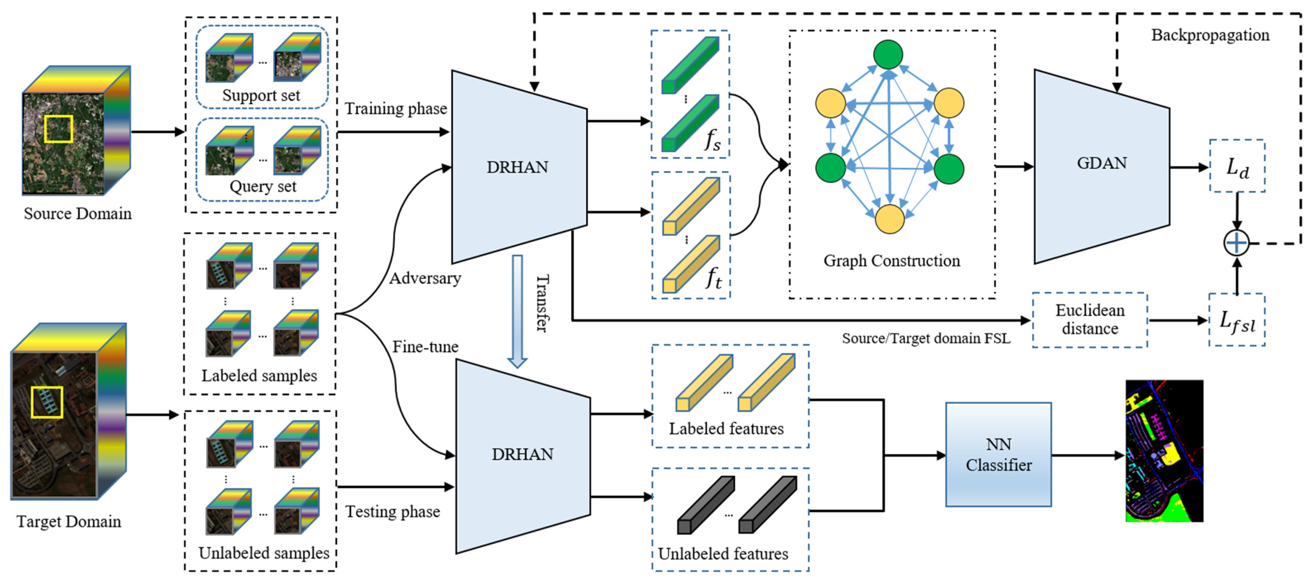
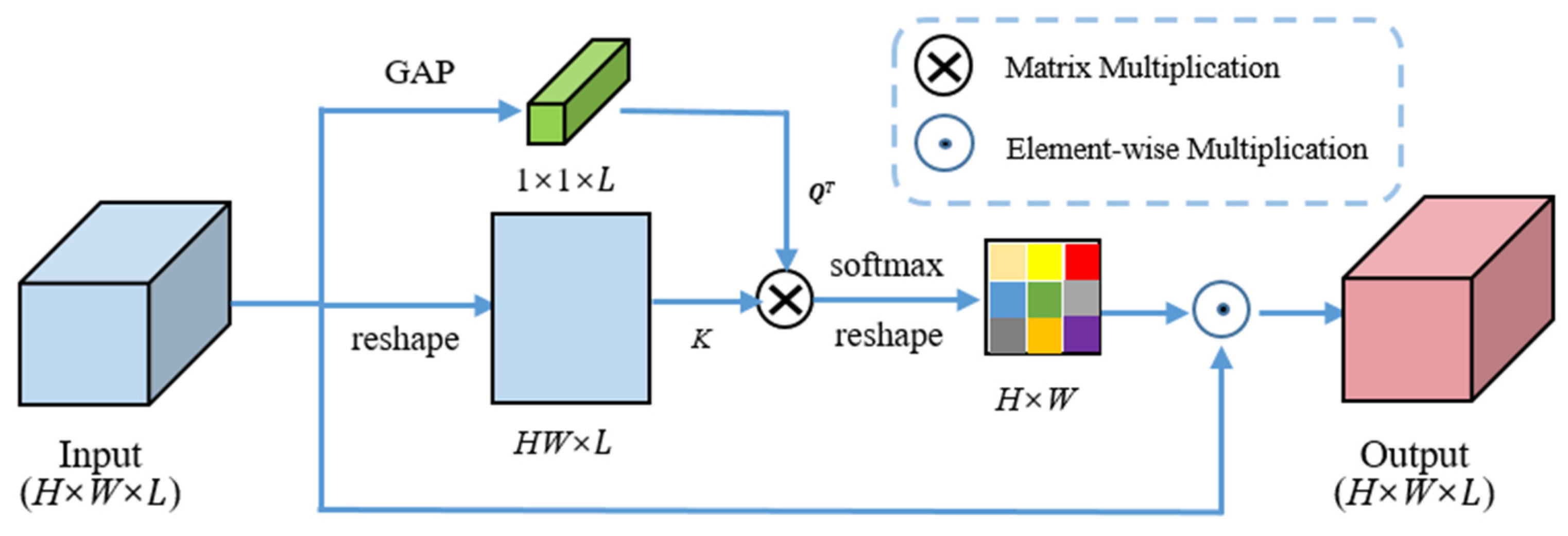
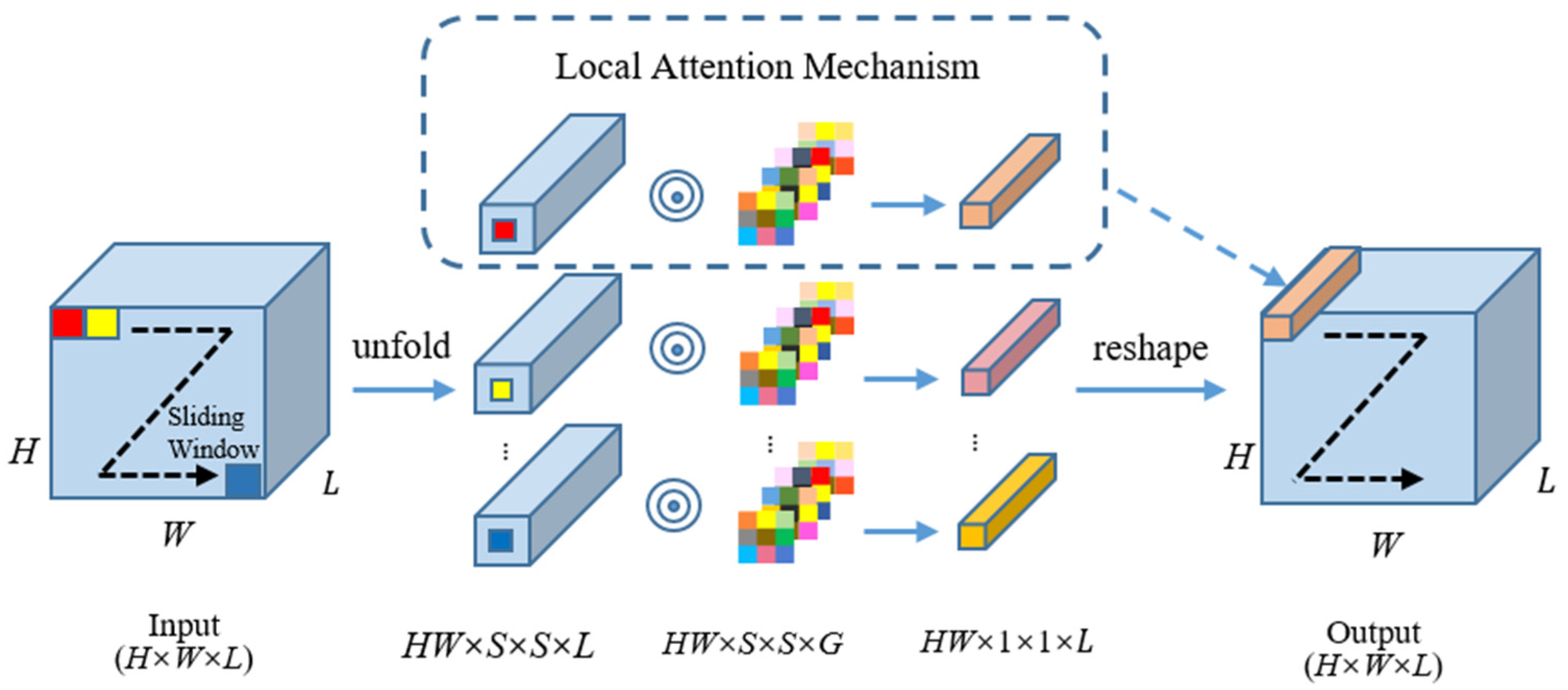
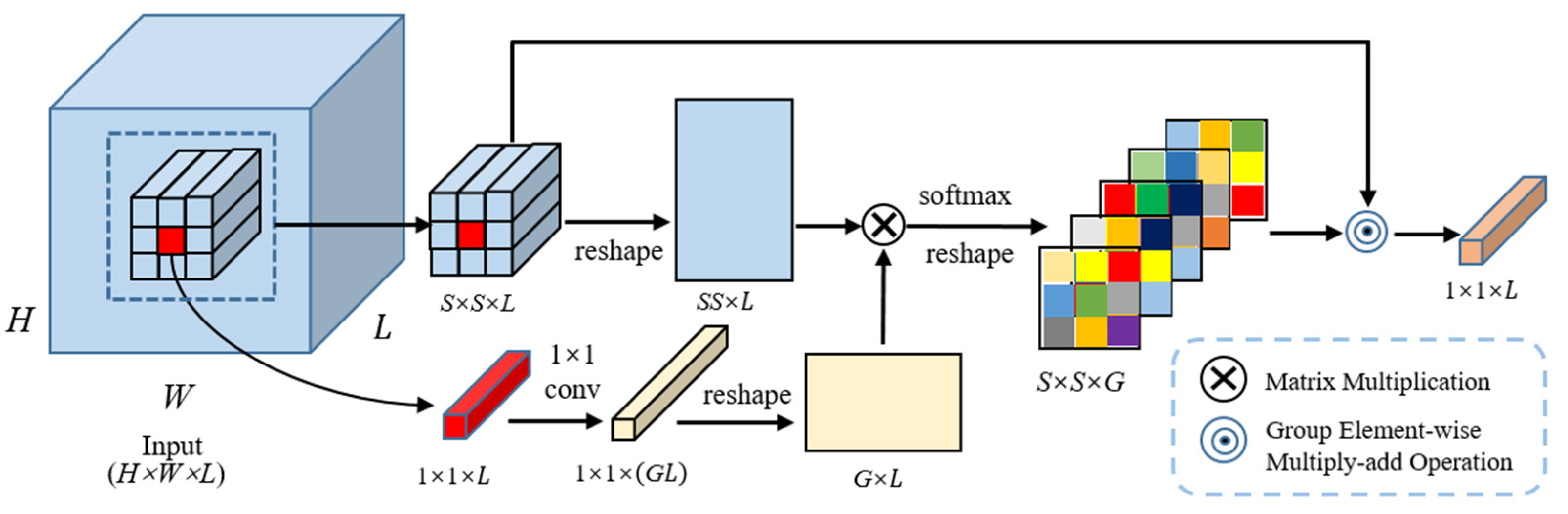
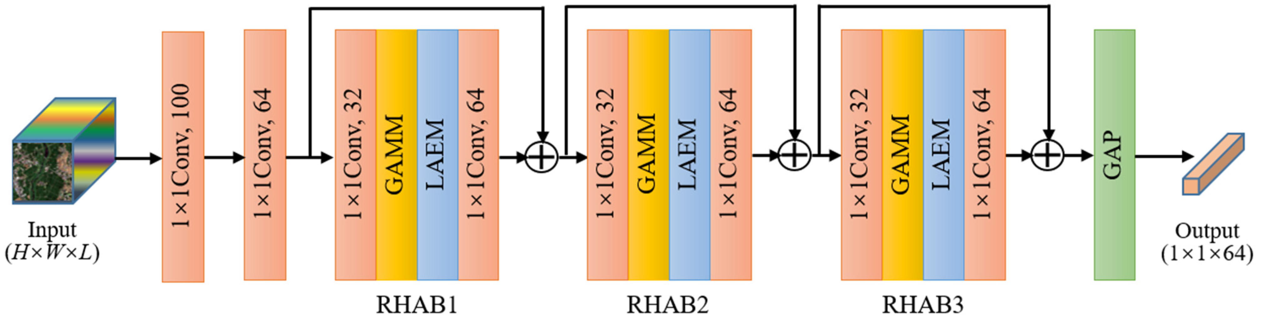
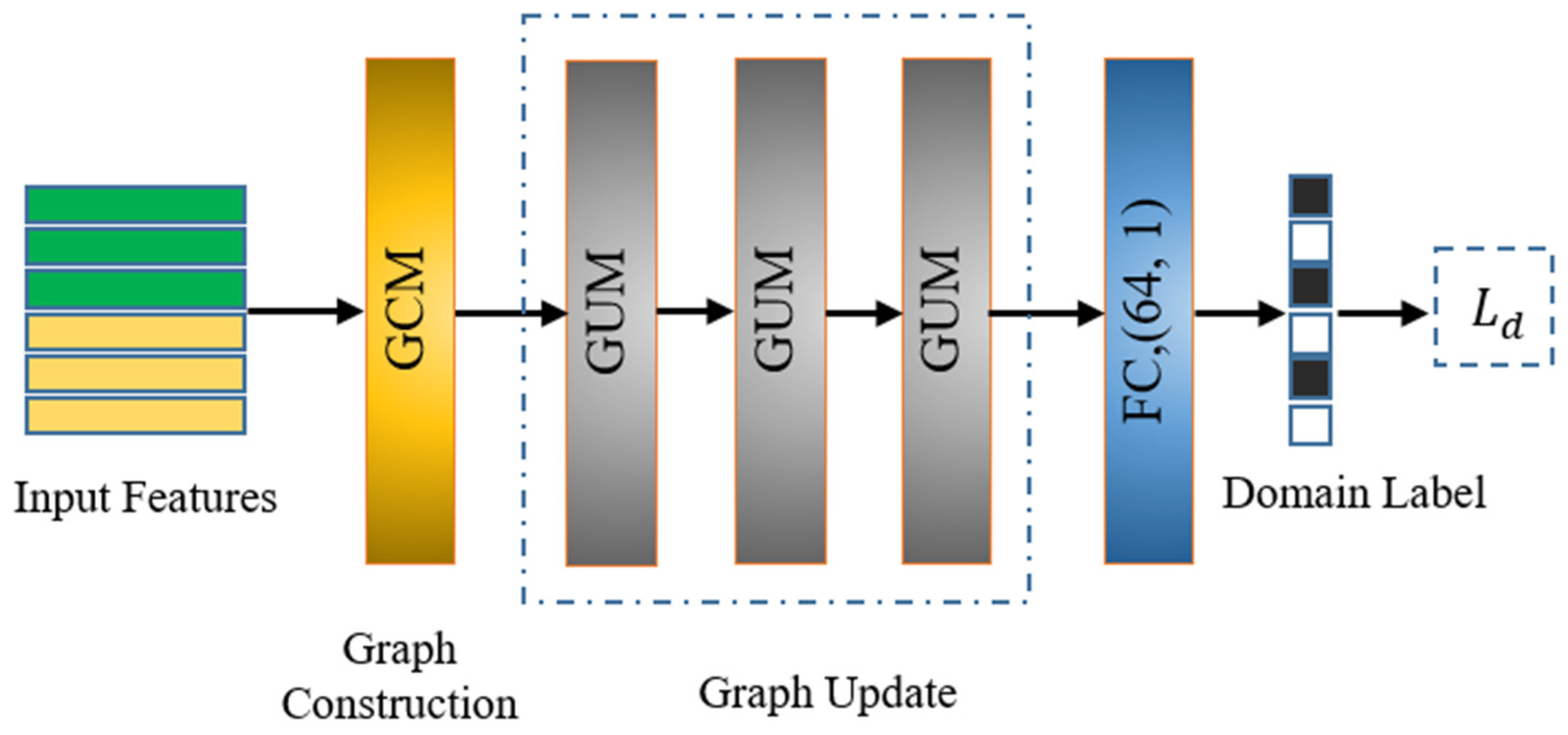
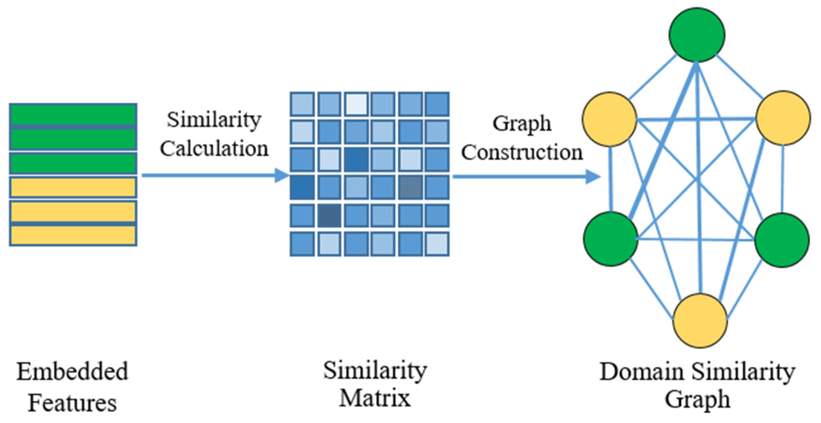
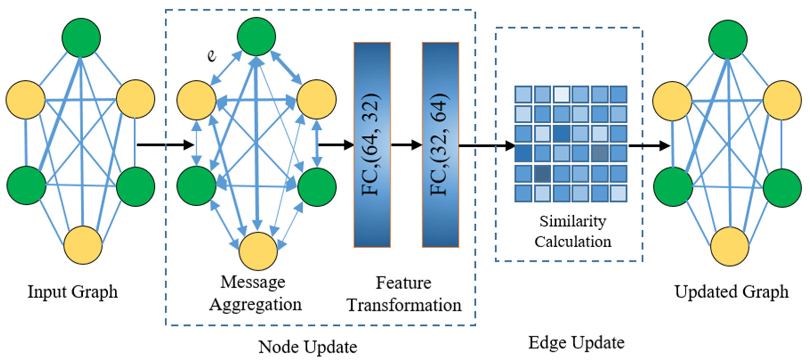
Although those abovementioned FSL methods achieved satisfactory classification performance with limited training samples, they are generally based on the hypothesis that both source and target domain datasets have the same data distribution. However, in practice scenarios, due to the difference in imaging mechanism, samples from the source and target domain may possess unique data characteristics and object categories. In this article, a novel graph-based domain adaptation FSL (GDAFSL) framework is developed to tackle these issues. Specifically, a deep residual hybrid attention network (DRHAN) is first proposed to learn a compact metric space. In this metric space, the embedding features extracted by DRHAN have a small intraclass distance and a large interclass distance. This means that the embedding features extracted by DRHAN are more compact within the same class and separate away from the other classes. Then, a few-shot HSI classification is performed on the learned compact metric space by calculating the Euclidean distance between class prototypes and unlabeled samples. In order to tackle the domain-shift problems, a novel graph-based domain adaptation network (GDAN) is proposed to align domain distribution and learn domain-invariant feature transformation. Benefits from the powerful ability of graphs to model complex interactions between nodes, a graph convolutional network (GCN) is embedded into the domain adversarial framework to explore the domain correlations between node features. The domain correlations are adopted as edge weights to guide the update of node features. Different from the ordinary feature-based domain adversarial strategy, the proposed method can more properly model domain correlations between samples with non-Euclidean characteristics structure and guide the optimization of learnable parameters to enhance the domain adaptation ability of deep models. In addition, the training process of GDAFSL follows a fashion of meta-learning to better simulate few-shot scenarios in practice. The experimental results conducted on three public HSI datasets prove that GDAFSL is outperforming other ordinary deep learning methods and state-of-the-art FSL methods. The main contribution of this article are as follows: (1) A novel DRHAN, which utilizes an attention mechanism to emphasize critical spatial features at a global scale and extract specific spatial features at a local scale, is proposed to enhance the capability of feature representation with limited labeled samples. (2) A novel graph-based domain adaptation network (GDAN) is proposed to achieve domain adaptation FSL. The GDAN utilizes graph construction to measure the domain correlations and generates more refined domain adaptation loss to guide the domain adaptation learning process. (3) A novel similarity measurement method is proposed to model the cross-domain correlations. The proposed method can aggregate node features more properly to obtain a more refined domain similarity graph for GDAN. (4) The proposed GDAFSL combines the FSL and graph-based domain adaptation method organically to improve the cross-domain few-shot classification performance. Extensive experiments conducted on three HSI datasets demonstrate the effectiveness of the proposed GDAFSL.

The remainder of this article is organized as follows. Section 2 reviewed some related works of GCNs and cross-domain FSL. Section 3 elaborates on the proposed GDAFSL. Section 4 reports the experimental results and analysis on three HSI datasets. Section 5 gives a further discussion about the classification performance of our method. Section 6 summarizes this article and draws a conclusion.

2. Related Works

In this section, related works of HSI classification are briefly reviewed. Meanwhile, the most relevant work of GCN and cross-domain FSL are reviewed in detail.

2.1. Graph Convolutional Network

In recent years, benefitting from the impressive representation ability of graph structure, GCNs have been widely applied in HSI classification [37,38,39,40,41] and achieved great success. A novel mini-batch-based GCN [37] is proposed to reduce the computation cost of large-scale HSIs in a mini-batch paradigm. Wan et al. [38] designed a dual interactive GCN (DIGCN) to capture spatial context information at different scales, which utilizes multiscale spatial interactions to refine node features and edge information in graphs. To classify unknown classes with small sample size, Zuo et al. [41] designed an edge-labeling graph neural network (FSL-EGNN) for few-shot HSI classification, which is the first attempt to combine GCN with FSL in a uniform framework. The FSL-EGNN exploits graph construction to model the associations between support set and quire set samples and utilizes edge labels to predict sample labels. Although GCN-based methods made a great success in HSI classification, they generally assume that both training and testing samples obey the same data distribution, ignoring the data and label distinction between different domains. In this work, a graph-based cross-domain FSL method is proposed to tackle the domain shift problems.

2.2. Cross-Domain FSL

Cross-domain FSL is an effective strategy to tackle the data and label shift problem between different data domains. Li et al. [42] designed a deep cross-domain few-shot learning (DCFSL) method which is the first attempt to combine FSL with domain adaptation and jointly realized cross-domain few-shot HSI classification in a unified framework. In the DCFSL framework, a spectral-spatial 3-D residual network is firstly designed to learn feature representation space for few-shot HSI classification. Then, a domain adversarial strategy is exploited to develop a domain invariant feature transformation for few-shot HSI classification. Bai et al. [43] introduced feature transformation into FSL to learn a diverse feature space with limited labeled samples and utilized a subspace classifier to classify testing data. Although obtaining satisfactory classification performance, these domain adaptation methods ignored the domain correlation between different domain samples which could reflect the deviation of domain distribution. In this article, a graph-based domain adaptation method, utilizing a domain similarity graph to model the deviations between source and target domain distributions, is proposed to guide models to develop a domain adaptation feature space.

3. Materials and Methods

In cross-domain HSI classification, the source and target domain datasets are generally from different scenes and captured by different sensors, which results in the variation in object categories and the specificity of spectral characteristics between different data domains. The samples from different data domains, which have non-Euclidean structural characteristics, are hard to model in a Euclidean space with ordinary metric methods. Therefore, a graph-based domain adversarial FSL method (GDAFSL) which utilizes graph construction to model the domain correlations and guide the domain adaptation learning process, is proposed to learn a domain invariant feature space under the cross-domain few-shot condition. The overall framework of GDAFSL is depicted in Figure 1.

3.1. Overview of the GDAFSL

To better illustrate the proposed GDAFSL for HSI classification, several relevant concepts are defined in this part. In the cross-domain FSL framework, the entire learning process contains two phases: the source domain training phase and the target domain fine-tuning phase. Specifically, the source domain training phase is first conducted on the source domain dataset ${\mathit{D}}_S$ in a meta-learning paradigm. Then, the pre-trained models are transferred to the target domain and perform few-shot classification on the target domain dataset ${\mathit{D}}_T$. Generally, the number of classes in ${\mathit{D}}_S$ is larger than that of ${\mathit{D}}_T$ to better construct meta-learning tasks. Due to the lack of labeled samples in the target domain, few labelled samples are selected in ${\mathit{D}}_T$ to form the target fine-tuning dataset ${\mathit{D}}_T^f$ and the remainder of unlabeled samples are regarded as testing dataset ${\mathit{D}}_T^t$, where ${\mathit{D}}_T^f{\displaystyle \cup }{\mathit{D}}_T^t={\mathit{D}}_T$, ${\mathit{D}}_T^f{\displaystyle \cap }{\mathit{D}}_T^t=\mathsf{\varnothing }$. In FSL methods, the training processes are iteratively conducted on a series of C-way-K-shot tasks, which are also called training episodes. In a training episode, C classes are first selected from the source domain ${\mathit{D}}_S$ and then K-labeled samples per class are randomly selected to construct the support set $\mathit{S}$ [42]. Similarly, another Z different unlabeled samples are also randomly selected from the same C classes in ${\mathit{D}}_S$ to construct the query set $\mathit{Q}$, where $\mathit{S}={\left\{(x_i,y_i)\right\}}_{i=1}^{C\times K}$, $\mathit{Q}={\left\{(x_j,y_j)\right\}}_{j=1}^{C\times Z}$ and $\mathit{S}{\displaystyle \cap }\mathit{Q}=\mathsf{\varnothing }$.

In GDAFSL, the entire FSL training phase includes two parts: FSL training process and the graph-based domain adaptation process. Specifically, FSL tasks are firstly constructed and fed through the feature extractor DRHAN to obtain discriminative semantic features. Then, metric learning methods are performed on these embedded features to generate few-shot classification results and calculate FSL loss $L_{fsl}$. After that, both source and target embedded features are utilized to construct a domain similarity graph. A novel graph-based domain adaptation network (GDAN) is designed to perform a domain adaptation process on a domain similarity graph and calculate domain adaptation loss $L_{\mathit{d}}$. Finally, the $L_{fsl}$ and $L_{\mathit{d}}$ are combined to jointly optimize the deep model via backpropagation.

In the FSL testing phase, the fine-tuning datasets ${\mathit{D}}_T^f$ are firstly utilized to fit a simple NN classifier. Then, the trained DRHAN and NN classifier are adopted to perform few-shot classification on the testing dataset ${\mathit{D}}_T^t$.

In addition, following the training strategy adopted in DCFSL [42], both source and target domain samples are exploited to train the DRHAN in an iterative manner. While one domain dataset is adopted to execute training procedure, another is regarded as the domain adversarial dataset to execute domain classification.

3.2. Feature Embedding with DRHAN

In this work, a novel deep residual hybrid attention network (DRHAN), which utilizes self-attention to model spatial interaction at global and local scales, is introduced to fully utilize context information in different spatial scales and efficiently extract discriminative semantic features with limited labeled samples.

3.2.1. Global Attention Mask Module

To fully utilize global context information and inhibit irrelevant information in an HSI patch, a novel global attention mask module (GAMM) which utilizes self-attention to model the spatial correlation between global feature representation and pixel vectors is proposed to generate a similarity mask. Those pixel vectors with larger similarity values play a more important role in feature extraction and vice versa. In this way, the relevant information is enhanced and irrelevant information is inhibited. The structure of GAMM is presented in Figure 2.

To acquire compact and precise feature representation of the input feature $\mathit{X}\in R^{H\times W\times L}$, global average pooling operation is firstly performed on $\mathit{X}$ to obtain a global average vector ${\mathit{d}}_{avg}$, as conducted in [44]. The ${\mathit{d}}_{avg}$ can be formulated as follow:

$${\mathit{d}}_{avg}=\frac{1}{H\times W}{\displaystyle \sum }_{i=1}^H{\displaystyle \sum }_{j=1}^W{\mathit{X}}_{i,j}\in R^{1\times 1\times L}.$$

(1)

The ${\mathit{d}}_{avg}$ is regarded as the query tensor to execute self-attention. Then, $\mathit{X}$ and ${\mathit{d}}_{avg}$ are reshaped to a matrix with a size of $HW\times L$ and a matrix with a size of $1\times L$, respectively. The similarity mask $\mathit{M}$ can be calculated by

$$\mathit{M}=\mathrm{softmax}\left(\left(\frac{\mathit{X}}{{\Vert \mathit{X}\Vert }_2}\right){\left(\frac{{\mathit{d}}_{avg}}{{\Vert {\mathit{d}}_{avg}\Vert }_2}\right)}^T\right)\in R^{HW\times 1},$$

(2)

where ${\Vert ·\Vert }_2$ denotes the $L_2$-norm along the spectral dimension. After that, $\mathit{M}$ is reshaped to a matrix with the size of $H\times W$ and executed element-wise multiplication with $\mathit{X}$ in each spectral dimension. The final output ${\mathit{X}}^{\prime }$ of GAML can be calculated by

$${\mathit{X}}_{i,j,k}^{\prime }={\mathit{X}}_{i,j,k}{\mathit{M}}_{i,j}.$$

(3)

3.2.2. Local Attention Encoding Module

In order to extract discriminative features with limited labeled samples, a novel local attention encoding module (LAEM) is proposed, which utilizes self-attention to model specific spatial interaction in a pixel neighborhood at different spatial locations. Inspired by the involution operators [45] which are spatial-specific and channel-agnostic feature kernels, we combine self-attention with involution operators to construct specific attention kernels for deep feature extraction. The structure of LAEM is presented in Figure 3.

For the input feature ${\mathit{X}}^{\prime }$ which is generated by GAML, the sliding windows operation is first executed on it to perform resample procedure. The spatial size and stride of sliding windows operation are set to $S\times S$ and 1, respectively. After that, the input feature is transformed into a set of local pixel blocks. These sliding local blocks can be easily extracted by using the unfolding technique in Pytorch. The local pixel blocks set can be defined as $\mathit{B}=\left\{{\mathit{B}}_{1,1},{\mathit{B}}_{1,2},\dots ,{\mathit{B}}_{H, W}\right\}\in R^{H\times W\times S\times S\times L}$, where ${\mathit{B}}_{i,j}\in R^{S\times S\times L}$ and ${\mathit{X}}_{i,j}^{\prime }\in R^{1\times 1\times L}$ is the center pixel of ${\mathit{B}}_{i,j}$. Then, a local attention mechanism (LAM) is adopted to generate specific attention kernels. The flowchart of LAM is presented in Figure 4.

Due to the positive effect of multihead attention mechanism to capture diverse semantic features, ${\mathit{X}}_{i,j}^{\prime }$ is mapped into a high-dimensional feature space to generate the multihead query ${\mathit{q}}_{i,j}$, which can be formulated as

$${\mathit{q}}_{i,j}=f\left({\mathit{W}}_Q, X_{i,j}^{\prime }\right)\in R^{1\times 1\times \left(GL\right)},$$

(4)

where $f(·)$ denotes the $1\times 1$ convolutional layer with weights ${\mathit{W}}_Q\in R^{\left(GL\right)\times L}$, and $G$ is the number of local attention kernels. After that, the matrix multiplication is performed on ${\mathit{q}}_{i,j}$ and ${\mathit{B}}_{i,j}$ to acquire attention kernels. The local attention kernels ${\mathit{A}}_{i,j}$ can be formulated as follows:

$${\mathit{A}}_{i,j}=\mathrm{softmax}\left(\left(\frac{{\mathit{B}}_{i,j}}{{\Vert {\mathit{B}}_{i,j}\Vert }_2}\right){\left(\frac{{\mathit{Q}}_{i,j}}{{\Vert {\mathit{Q}}_{i,j}\Vert }_2}\right)}^T\right)\in R^{SS\times G}.$$

(5)

The local attention kernels set can be defined as $\mathit{A}=\left\{{\mathit{A}}_{1,1},{\mathit{A}}_{1,2},\dots ,{\mathit{A}}_{H, W}\right\}\in R^{H\times W\times S\times S\times G}$, where ${\mathit{A}}_{i,j}\in R^{S\times S\times G}$. To obtain the final feature maps ${\mathit{X}}^{″}\in R^{H\times W\times L}$, these local attention kernels ${\mathit{A}}_{i,j}$ are applied on the corresponding pixel blocks ${\mathit{B}}_{i,j}$ and executed element-wise multiply-add operations. The ${\mathit{X}}^{″}$ can be formulated as follows:

$${\mathit{X}}_{i,j,k}^{″}={\displaystyle \sum }_{p=1}^S{\displaystyle \sum }_{q=1}^S{\mathit{A}}_{i,j,p,q,kG/L}{\mathit{B}}_{i,j,p,q,k}.$$

(6)

3.2.3. Deep Residual Hybrid Attention Network

The architecture of the proposed feature extractor DRHAN is presented in Figure 5. As shown in Figure 5, the proposed DRHAN is composed of two $1\times 1$ convolutional layers, three hybrid attention residual blocks (RHABs), and a global average pooling layer. The first $1\times 1$ convolutional layer is responsible for mapping the HSIs into a dimension-fixed feature space to ensure that all input HSIs have a uniform spectral dimension before performing feature extraction, which is also named as mapping layer [46]. The second $1\times 1$ convolutional layer is responsible for the feature dimension reduction of the mapping layer’s output. The three RHABs utilized to extract discriminative semantic features are constructed by embedding GAMLs and LAEMs into ordinary residual blocks. The final global average pooling layer is responsible for feature integration to acquire a compact feature representation for the following few-shot classification. In this work, the spatial size of sliding windows $S$ and the number of local attention kernels $G$ is set to 3 and 16, respectively.

3.3. Few-Shot Classification for HSI

In the FSL framework, metric learning methods are generally adopted to perform few-shot classification. Given a C-way-K-shot task, the feature extractor is first adopted to extract discriminative semantic features. Then, a softmax-based distance metric method is adopted to measure the probability distribution of query samples in FSL tasks. The class probability of query sample $\mathit{x}$ can be formulated as

$$P\left(\left(y=l|\mathit{x}\in \mathit{Q}\right)\right)=\frac{\exp \left(-d\left(F_{\phi }\left(\mathit{x}\right),{\mathit{c}}_l\right)\right)}{{{\displaystyle \sum }}_{l=1}^C\exp \left(-d\left(F_{\phi }\left(\mathit{x}\right),{\mathit{c}}_l\right)\right)},$$

(7)

where $d(·)$ denotes Euclidean distance metric, $F_{\phi }(·)$ denotes the feature extractor. ${\mathit{c}}_l$ is the class prototype of the lth class in $\mathit{Q}$, the ${\mathit{c}}_l$ can be calculated as follows:

$${\mathit{c}}_l=\frac{1}{N_l}{\displaystyle \sum }_{h=1}^{N_l}{F}_{\phi }\left({\mathit{x}}_h\right),$$

(8)

where $N_l$ denotes the number of samples in lth class. Then, the FSL classification loss function $L_{fsl}$ can be defined as

$$L_{fsl}=-\frac{1}{N_{\mathit{Q}}}{\displaystyle \sum }_{\left(x, y\right)\in \mathit{Q}}{\displaystyle \sum }_{l=1}^{C}1\left\{l=y\right\}\log P\left(\left(y=l|\mathit{x}\right)\right),$$

(9)

where $N_{\mathit{Q}}$ denotes the number of samples in query set Q. $1\left\{l=y\right\}$ is an indicator function. It means that if $l$ is equal to $y$, the value of the function is 1; otherwise, its value is 0.

3.4. Graph Domain Adaptation Network

In order to explore the domain correlations and learn a domain invariant metric space, a graph domain adaptation network (GDAN) is proposed, which explicitly updates the domain correlation graph and utilizes it to guide the domain adaptation process. Specifically, the GDAN consists of a graph construction module (GCM), three graph update modules (GUMs), and a fully connected layer. Specifically, the GCM is first utilized to construct an initial domain similarity graph from embedded features. Then, three GUMs are stacked to explicitly update node features and edge weights of the graph. Finally, the FC is responsible for executing domain distinction on those updated node features to obtain domain labels. The structure of GDAN is presented in Figure 6.

3.4.1. Graph Construction Module

The flowchart of GCM is presented in Figure 7. In the domain similarity graph, each embedded feature of source and target domains is regarded as a graph node feature and the domain similarities between embedded features are regarded as graph edge weights. Due to the non-Euclidean structural characteristic of cross-domain data, general similarity metric methods for Euclidean spaces (i.e., cosine similarity) cannot properly model their domain correlations. In this work, the KL divergence, which is generally utilized to measure the divergence between two probability distributions, is adopted to calculate domain similarity. For the sample in source domain distribution $P_s\left(x\right)$ and target domain distribution $P_t\left(x\right)$, given its corresponding graph node feature ${\mathit{V}}_m\in R^{1\times 1\times L}$, its statistical probability vector can be expressed as

$${\mathit{p}}_m=\mathrm{softmax}\left({\mathit{V}}_m\right)\in R^{1\times 1\times L}.$$

(10)

The KL divergence of the probability statistics vector ${\mathit{p}}_m$ and ${\mathit{p}}_n$ can be calculated as

$$d\left({\mathit{p}}_m\Vert {\mathit{p}}_n\right)={\displaystyle \sum }_{k=1}^L{p}_m^k\ln \frac{p_m^k}{p_n^k},$$

(11)

where $p_m^k$ and $p_n^k$ denote the element value in the kth spectral dimension of ${\mathit{p}}_m$ and ${\mathit{p}}_n$, respectively. As the KL divergence between ${\mathit{p}}_m$ and ${\mathit{p}}_n$ is asymmetrical, that is, $d\left({\mathit{p}}_m\Vert {\mathit{p}}_n\right)\ne d\left({\mathit{p}}_m\Vert {\mathit{p}}_n\right)$. According to the cross entropy between probability statistics vectors, the domain correlation between the feature vector ${\mathit{V}}_m$ and ${\mathit{V}}_n$ can be formulated as

$$d_{KL}\left({\mathit{V}}_m\Vert {\mathit{V}}_n\right)=d\left({\mathit{p}}_m\Vert {\mathit{p}}_n\right)+d\left({\mathit{p}}_n\Vert {\mathit{p}}_m\right).$$

(12)

It is noteworthy that, KL divergence reflects the deviations between two distributions, the larger the value of $d_{KL}$ is, the lower the domain similarity between feature vectors, and vice versa. Therefore, $d_{KL}$ cannot be directly utilized as edge weights to perform message aggregation. In order to obtain a proper similarity coefficient, we transform the $d_{KL}$ as follows:

$$d_{sim}\left({\mathit{V}}_m\Vert {\mathit{V}}_n\right)=\mathrm{softmax}\left(-d_{KL}\left({\mathit{V}}_m\Vert {\mathit{V}}_n\right)\right).$$

(13)

Then, the edge weights matrix $\mathit{E}$ of the whole graph can be formulated as

$$\mathit{E}=\left[\begin{array}{cc}{d}_{sim}\left({\mathit{V}}_1\Vert {\mathit{V}}_1\right)& \begin{array}{ccc}{d}_{sim}\left({\mathit{V}}_1\Vert {\mathit{V}}_2\right)& \cdots & d_{sim}\left({\mathit{V}}_1\Vert {\mathit{V}}_{N_G}\right)\end{array}\\ \begin{array}{c}{d}_{sim}\left({\mathit{V}}_2\Vert {\mathit{V}}_1\right)\\ ⋮\\ d_{sim}\left({\mathit{V}}_N\Vert {\mathit{V}}_1\right)\end{array}& \begin{array}{ccc}{d}_{sim}\left({\mathit{V}}_2\Vert {\mathit{V}}_2\right)& \cdots & d_{sim}\left({\mathit{V}}_2\Vert {\mathit{V}}_{N_G}\right)\\ ⋮& \ddots & ⋮\\ d_{sim}\left({\mathit{V}}_N\Vert {\mathit{V}}_2\right)& \cdots & d_{sim}\left({\mathit{V}}_N\Vert {\mathit{V}}_{N_G}\right)\end{array}\end{array}\right],$$

(14)

where $N_{\mathit{G}}$ denotes the number of nodes in a graph. The node features and edge weights are combined to construct the domain similarity graph.

3.4.2. Graph Update Module

In order to fully explore domain correlations and learn a domain invariant feature transformation, a graph update module (GUM) is introduced to explicitly update the domain similarity graph. The architecture of GUM is presented in Figure 8.

The GUM contains two procedures: node update and edge update. Specifically, given an input graph $\mathit{G}$ with node features $\mathit{V}$ and edge weights $\mathit{E}$, the message aggregation mechanism is firstly executed to aggregate features of adjacent nodes. Then, the aggregated node features are fed through two fully connected layers to perform feature transformation. The updated node features ${\mathit{V}}^{\prime }$ can be formulated as

$${\mathit{V}}_m^{\prime }=f\left({\mathit{W}}_2,f\left({\mathit{W}}_1,{\displaystyle \sum }_{n=1}^N{\mathit{E}}_{m,n}{\mathit{V}}_n\right)\right)\in R^{1\times 1\times L},$$

(15)

where $f(·)$ denotes the fully connected layer, ${\mathit{W}}_1\in R^{L\times L^{\prime }}$ and ${\mathit{W}}_2\in R^{L^{\prime }\times L}$ are learnable parameters of the two fully connected layers, respectively. After that, according to Equations (7)–(11), the domain similarity matrixes of ${\mathit{V}}^{\prime }$ are recalculated to obtain the updated edge weights ${\mathit{E}}^{\prime }$. Finally, the ${\mathit{V}}^{\prime }$ and ${\mathit{E}}^{\prime }$ are utilized to construct the updated graph ${\mathit{G}}^{\prime }$.

3.4.3. Graph Domain Discriminator

After several iterations of GUM, the domain correlations between samples of source and target domain have been fully explored. The domain discriminative node features in the graph are fed through a domain discriminator which consists of a fully connected layer to predict domain labels. The domain adaptation loss function $L_{\mathit{d}}$ defined on the domain similarity graph $\mathit{G}$ can be formulated as

$$L_d=-\frac{1}{N_{\mathit{G}}}{\displaystyle \sum }_{m=1}^{N_{\mathit{G}}}\left[y_{{\mathit{V}}_m}\log \Theta \left({\mathit{V}}_m\right)+\left(1-y_{{\mathit{V}}_m}\right)\log \left(1-\Theta \left({\mathit{V}}_m\right)\right)\right],$$

(16)

where $\Theta (·)$ denotes the predicted probability that the sample corresponding to ${\mathit{V}}_m$ is from the source domain, $y_{{\mathit{V}}_m}$ denotes the true domain label of the sample corresponding to ${\mathit{V}}_m$. $N_{\mathit{G}}$ denotes the number of nodes in graph $\mathit{G}$. As the domain distinction is a binary classification task, the true domain labels of source and target domain samples are set to 1 and 0, respectively.

Therefore, the domain adversarial loss function can be refined as

$$L_d=-\frac{1}{N^S}{\displaystyle \sum }_{r=1}^{N^S}\log \Theta \left({\mathit{V}}_r^S\right)-\frac{1}{N^T}{\displaystyle \sum }_{t=1}^{N^T}\log \left(1-\Theta \left({\mathit{V}}_t^T\right)\right),$$

(17)

where $N^S$ and $N^T$ denote the number of training samples from the source and target domain, respectively.${\mathit{V}}_r^S$ and ${\mathit{V}}_t^T$ denote the node features corresponding to the source sample ${\mathit{x}}_r^S$ and target sample ${\mathit{x}}_t^T$, respectively. The GDAN minimizes the above loss function, while the DRHAN maximizes it. By performing such an adversarial learning process, a domain invariant metric space is gradually learned with limited labeled samples.

4. Experiments

4.1. Description of Experiment Datasets

To assess the classification performance of GDAFSL, several public HSI datasets, including the Chikusei dataset, the Indian Pines (IP) dataset, the University of Pavia (UP) dataset, and the Salina Valley (SV) dataset, are selected to conduct comprehensive experiments. As the proposed GDAFSL is a cross-domain FSL, the Chikusei dataset is adopted as the source domain dataset, and IP, UP, and SV datasets are regarded as the target domain dataset. Another reason to select the Chikusei dataset as the source domain dataset is that the spectral characteristics of the Chikusei dataset are different from the other three datasets, which can better verify the effectiveness of GDAFSL.

The Chikusei dataset, captured by hyperspectral visible/near-infrared cameras (Hyperspec-VNIR-C) in 2014, in Chikusei, Ibaraki, Japan, consists of 19 land-cover categories and a total of 77,592 labeled pixels. It has 2517 $\times$ 2335 pixels in spatial dimension and 128 spectral bands in spectral dimension. The corresponding wavelengths ranged between 363 and 1018 nm. Its spectral resolutions and ground sample distance (GSD) are 10nm and 2.5 m/pixel, respectively.

The Indian Pines dataset, captured by the airborne visible infrared imaging spectrometer (AVIRIS) sensor in 1992, over Indiana, USA, contains 16 object categories and a total of 10,249 labeled pixels. It has 145 $\times$ 145 pixels in spatial dimension and 200 spectral bands in spectral dimension. The corresponding wavelengths are ranged between 400 and 2500 nm. The spectral resolution and GSD of the IP dataset are 10nm and 20 m/pixel, respectively.

The University of Pavia dataset, captured by the reflective optics system imaging spectrometer (ROSIS) sensors over Pavia, Northern Italy, consists of nine land-cover categories and a total of 42,776 labeled pixels. It has 610 $\times$ 340 pixels in spatial dimension and 103 spectral bands in spectral dimension. The corresponding wavelengths are evenly distributed between 430 and 860 nm. The spectral resolution and GSD of the UP dataset are 4nm and 1.3 m/pixel, respectively.

The Salina Valley dataset, captured by the airborne visible/infrared imaging spectrometer (AVIRIS) sensors over Salinas Valley, CA, USA, consists of 16 land-cover categories and a total of 54,129 labeled pixels. It has 512 $\times$ 217 pixels in spatial dimension and 204 spectral bands in spectral dimension. The corresponding wavelength ranged between 400 and 2500 nm. The spectral resolution and GSD of the SV dataset are 10 nm and 3.7 m/pixel, respectively.

In our experiments, to ensure the balance of the number of training samples in various classes, 200 labeled samples per class are randomly selected from the source domain dataset to perform source FSL, as conducted in [30]. 5 labeled samples per class are also sampled from target domain datasets to construct fine-tuning dataset (training dataset) for target domain fine-tuning or target domain FSL.

Table 1. The Numbers of Training, Testing, and Total Samples in IP Dataset.

Class	Class Name	Train	Test	Total
1	Alfalfa	5	41	46
2	Corn-notill	5	1423	1428
3	Corn-mintill	5	825	830
4	Corn	5	232	237
5	Grass-pasture	5	478	483
6	Grass-trees	5	725	730
7	Grass-pasture-mowed	5	23	28
8	Hay-windrowed	5	473	478
9	Oats	5	15	20
10	Soybean-notill	5	967	972
11	Soybean-mintill	5	2450	2455
12	Soybean-clean	5	588	593
13	Wheat	5	200	205
14	Woods	5	1260	1265
15	Buildings-Grass-Trees-Drives	5	381	386
16	Stone-Steel-Towers	5	88	93
	Total	80	10,169	10,249

,

Table 2. The Numbers of Training, Testing, and Total Samples in UP Dataset.

Class	Class Name	Train	Test	Total
1	Asphalt	5	6626	6631
2	Meadows	5	18,644	18,649
3	Gravel	5	2094	2099
4	Trees	5	3059	3064
5	Painted metal sheets	5	1340	1345
6	Bare Soil	5	5024	5029
7	Bitumen	5	1325	1330
8	Self-Blocking Bricks	5	3677	3682
9	Shadows	5	942	947
	Total	45	42,731	42,776

and

Table 3. The Numbers of Training, Testing, and Total Samples in SV Dataset.

Class	Class Name	Train	Test	Total
1	Brocoli_green_weeds_1	5	2004	2009
2	Brocoli_green_weeds_2	5	3721	3726
3	Fallow	5	1971	1976
4	Fallow_rough_plow	5	1389	1394
5	Fallow_smooth	5	2673	2678
6	Stubble	5	3954	3959
7	Celery	5	3574	3579
8	Grapes_untrained	5	11,266	11,271
9	Soil_vinyard_develop	5	6198	6203
10	Corn_senesced_green_weeds	5	3273	3278
11	Lettuce_romaine_4wk	5	1063	1068
12	Lettuce_romaine_5wk	5	1922	1927
13	Lettuce_romaine_6wk	5	911	916
14	Lettuce_romaine_7wk	5	1065	1070
15	Vinyard_untrained	5	7263	7268
16	Vinyard_vertical_trellis	5	1802	1807
	Total	80	54,049	54,129

present the partitioning of IP, UP, and SV datasets, respectively.

Since the FSL training processes are performed alternately on source and target data sets, labeled samples in the target fine-tuning dataset are insufficient to construct target FSL tasks, and data augmentation methods are adopted to expand the target fine-tuning dataset. The samples of the original fine-tune dataset are firstly rotated 90, 180, and 270 degrees clockwise, respectively. Then, the Gaussian noise is randomly added to the rotated samples to further expand the target fine-tuning dataset. It is worth noting that the augmented dataset is only used for target domain FSL and the original fine-tuning dataset is only used to perform target domain fine-tuning.

4.2. Experimental Setup

In this article, our experiments are conducted on a workstation with an AMD Threadripper processor (2.90 GHz), 64 GB of memory, and an RTX 3090 graphics processing unit with 24 GB RAM. All HSI classification methods adopted in our experiments are constructed by utilizing Python language in the Pytorch platform.

In our experiments, the Adam optimizer is adopted to optimize learnable parameters. The Xavier normalization method is adopted to initialize convolutional kernels in GDAFSL. The initial learning rate is set to 0.001 and reduced by 5% after every 200 iterations. The training epoch of the FSL training process is set to 10,000. For a C-way-K-shot task in the FSL training process, C is set to the class number of the target dataset and K is set to 1. The query sample size Z of the query set $\mathit{Q}$ in each task is set to 19, as conducted in [30,31]. The overall accuracy (OA), average accuracy (AA), and Kappa coefficients (κ) are adopted to quantitatively evaluate different HSI classification methods. All methods are executed 10 times on three HSI datasets to calculate averages and standard deviations of OA, AA, and κ.

4.3. Parameters Setup

In this section, some main hyperparameters, the initial learning rate, the number of the epoch, the size of tasks in FSL, the neighborhood size P, and the number of GUM $N_{GU\mathit{M}}$, are discussed to find the optimal value for GDAFSL.

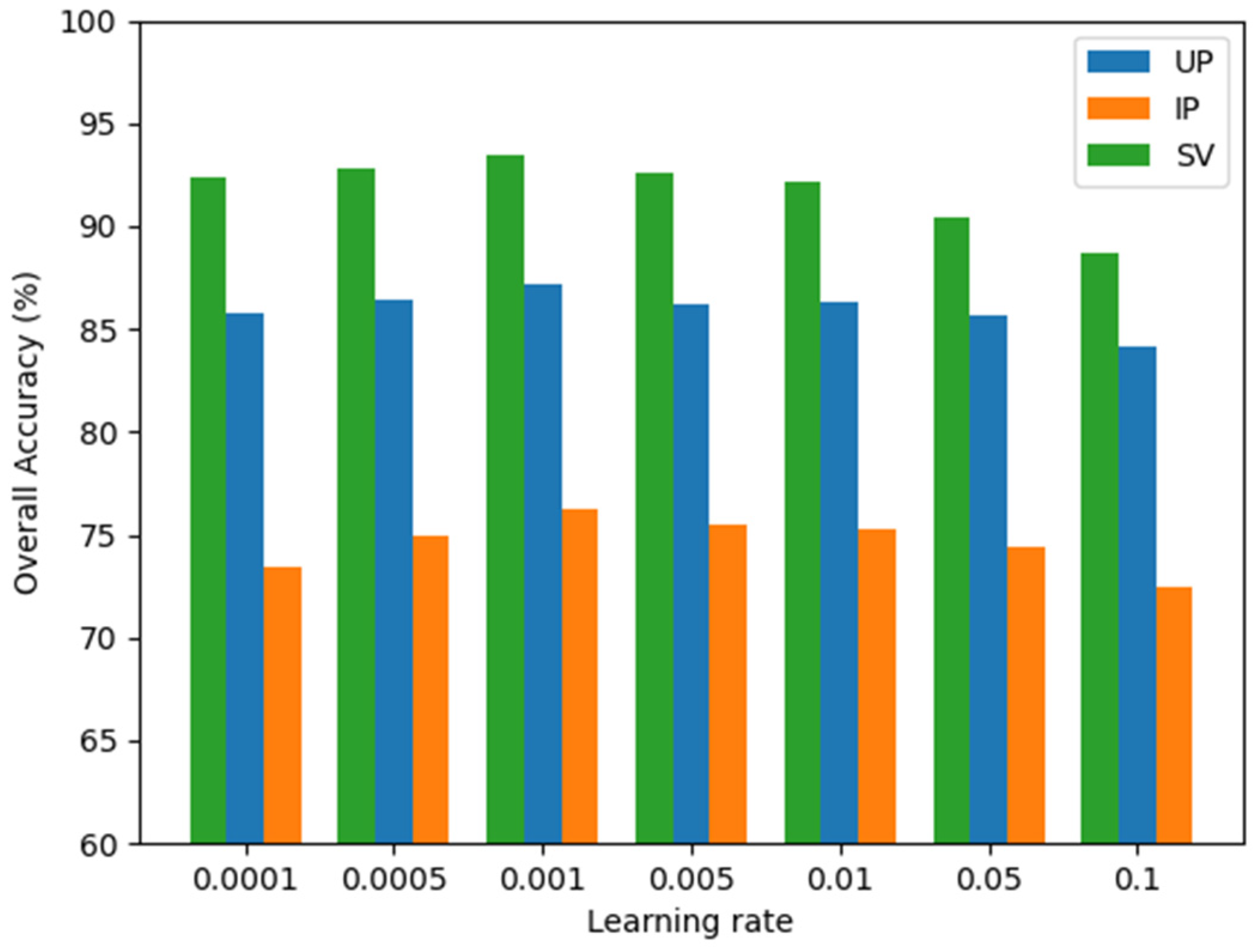
The learning rate plays an important role in the training process. To find the optimal initial learning rate, several experiments with different learning rates {0.0001, 0.0005, 0.001, 0.005, 0.01, 0.05, 0.1} are conducted on three target datasets. The experimental results are presented in Figure 9. When the initial learning rate is set to 0.001, GDAFSL achieved the best classification performance on three target datasets. The overlarge or overall learning rate, such as 0.1 or 0.0001, may cause the model cannot to converge to the optimal solution. Therefore, the initial learning rate is set to 0.001 and reduced by 5% after every 200 iterations.

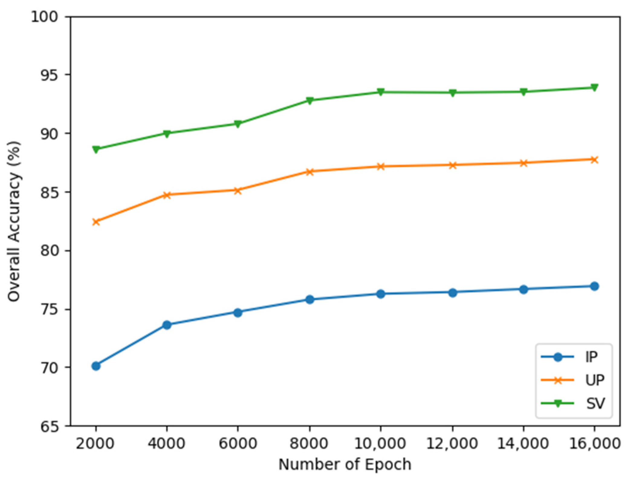
The number of the epoch is another vital parameter in the training process. To find the optimal value of it, we also conducted experiments with various numbers of epochs. The number of epochs are set as 2000, 4000, 6000, 10,000, 12,000, 14,000, and 16,000, respectively. The experimental results are presented in Figure 10. The OAs of GDAFSL on three datasets increased continuously with the increase of the number of epochs. When it reached 10,000, the OAs began to converge. Therefore, to balance the relationship between classification performance and time cost, the number of epochs is set to 10,000 on three target datasets.

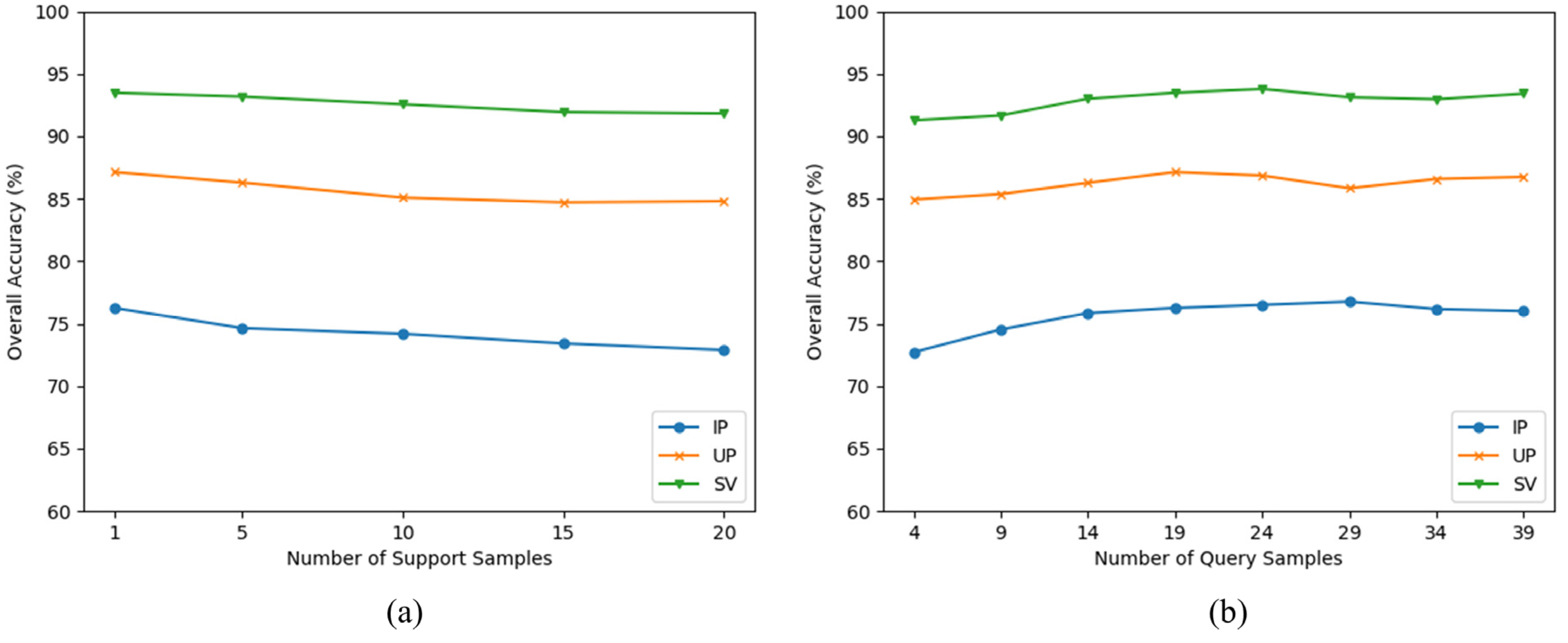
As mentioned in Section 3.1, the training processes of the FSL method are iteratively conducted on a series of C-way-K-shot tasks. The size of the task is also vital to the model’s classification performance. To find the optimal task size of GDAFSL, several experiments are conducted on three target datasets. Specifically, the number of support samples K and the number of query samples Z are discussed in this part. The K is set to 1, 5, 10, 15, and 20, respectively. The Z is set to 4, 9, 14, 19, 24, 29, 34, and 39, respectively. The experimental results are presented in Figure 11. When K is set to 1, the OAs reached the maximum. Then, the OAs decreased continuously with the increase of K. For the number of query samples Z, the OAs increased continuously with the increase of Z. When the Z is set to 19, the OAs start to converge. Therefore, the number of support samples K and the number of query samples Z are set to 1 and 19, respectively.

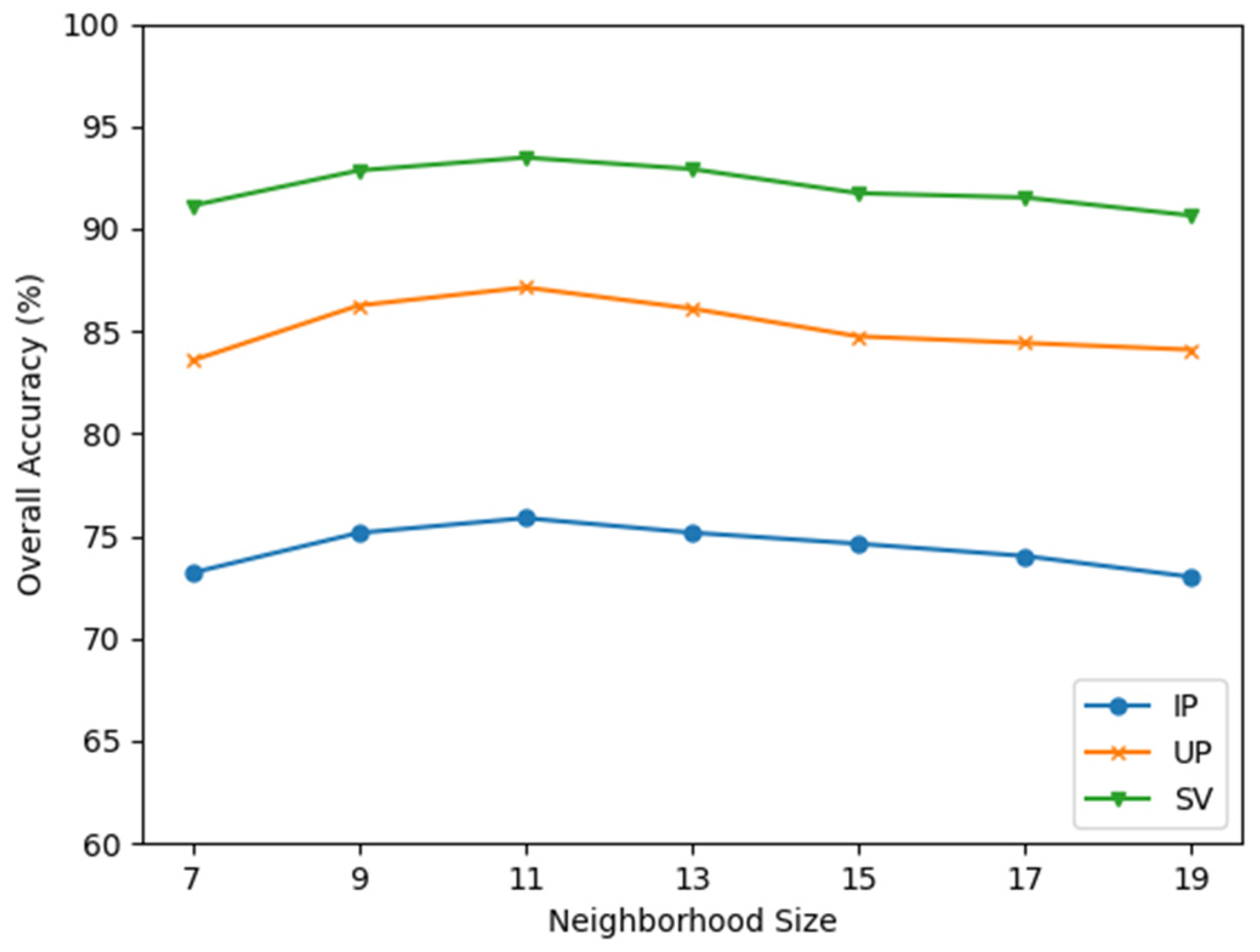
To utilize abundant spatial-spectral information in HSIs, HSI pixels are firstly sampled as $P\times P\times L$ pixel neighborhoods to perform HSI classification. Several experiments with different neighborhood sizes $\left\{7,9,11,13,15,17\right\}$ are conducted to find the optimal value of P on three HSI datasets. As exhibited in Figure 12, when $P$ is smaller than 11, the OAs of GDAFSL increased continuously with the increase of $P$. When $P$ is set to 11, GDAFSL achieved the best classification performance and acquired the highest OAs. While $P$ is larger than 11, with the increase of $P$, the OAs decreased continuously instead. We consider that properly expanding the spatial size of pixel neighborhoods generally has a positive impact on classification performance, but the too-large value of P will introduce irrelevant noises to weaken the classification performance of deep models. Therefore, the optimized neighborhood size is set to 11.

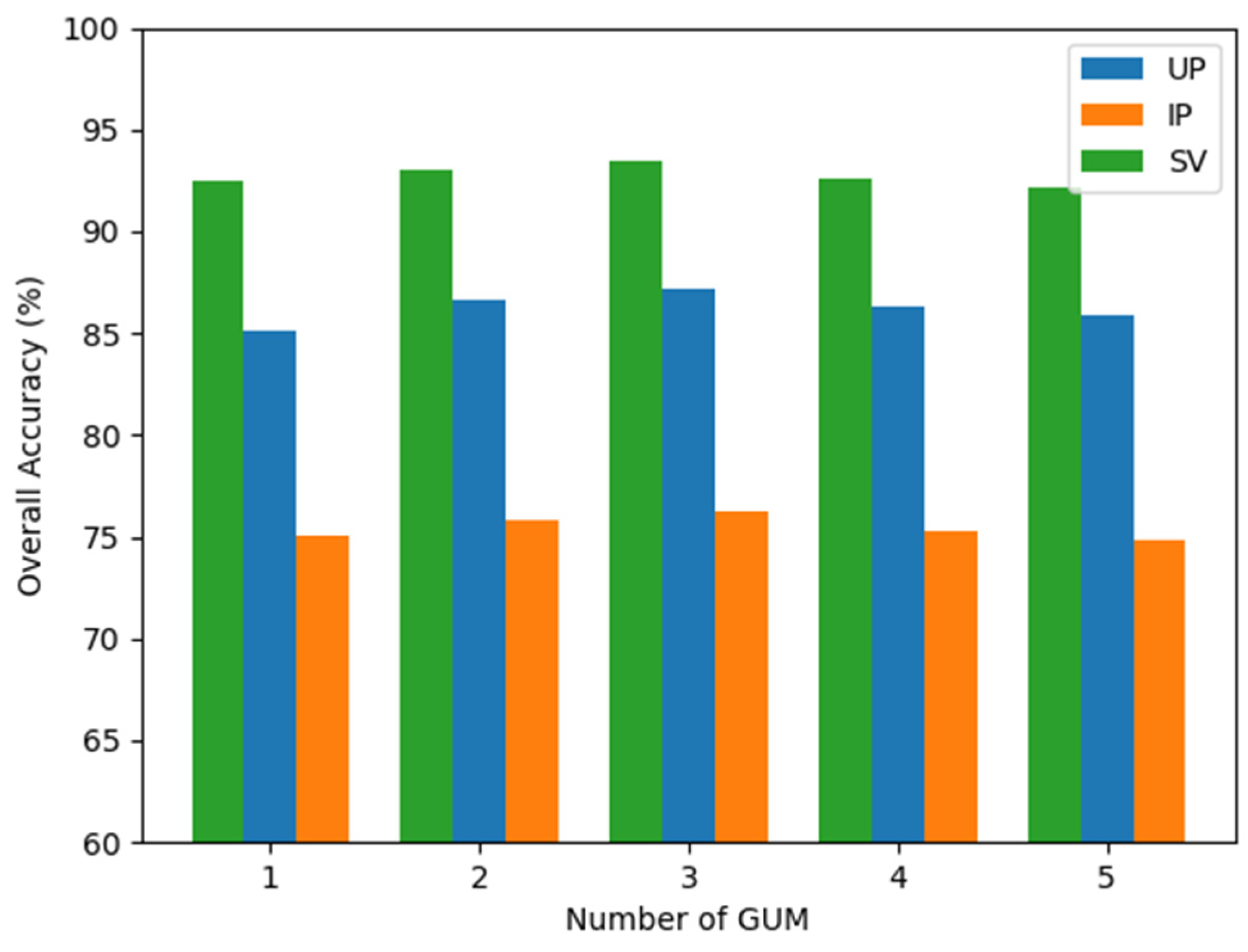
The number of GUM $N_{GU\mathit{M}}$ determines the ability of GDAN to explore domain correlations between different domain samples. To find the optimal value of $N_{GU\mathit{M}}$, several experiments are conducted with different numbers of GUM $\left\{1,2,3,4,5\right\}$. The experimental results are reported in Figure 13. With the increase of $N_{GU\mathit{M}}$, the OAs first increased and then decreased, and when $N_{GU\mathit{M}}$ is set to 3, the OAs reached the highest value. We consider that the appropriate deepening of GDAN helps to explore domain correlations, but the overly large value of $N_{GU\mathit{M}}$ will make GDAN too complex to be optimized properly, which weakens the capability of GDAN to model domain correlations. Therefore, the optimal value of $N_{GU\mathit{M}}$ is set to 3 in this work.

4.4. Ablation Studies

Comprehensive ablation studies are conducted on several target HSI datasets to assess the specifically designed modules in GDAFSL and evaluate their contributions to HSI classification. In this article, the ordinary residual CNN, which has a similar structure to DRHAN and utilizes 3 $\times$ 3 convolutional layers for feature extraction, is combined with the FSL method as a baseline HSI classification method.

4.4.1. The Impact of DRHAN

To evaluate the feature representation ability of the proposed feature extractor DRHAN, we gradually add GAMM and LAEM into the baseline and conduct experiments on three target datasets under the GDAFSL framework.

Table 4. OAs obtained by GDAFSL with various feature extraction modules on three target datasets.

Additional Module	IP	UP	SV
Baseline	65.58 ± 2.75	78.87 ± 2.19	87.21 ± 1.89
GAMM	69.21 ± 2.37	82.78 ± 2.27	89.61 ± 1.46
LAEM	71.67 ± 2.17	84.12 ± 2.31	90.86 ± 1.23
GAMM + LAEM	72.97 ± 2.40	84.53 ± 1.59	91.37 ± 1.01

presents the experimental results and the best classification results are shown in bold. Due to the lack of additional specific designed modules, the baseline method achieves the worst classification performance compared with other specific designed combinations. The combination of “GAMM + LAEM”, which is also called the DRHAN, achieves the best classification results on three target datasets. Compared with DRHAN, separately utilizing GAMM or LAEM cannot achieve competitive classification performance, and the performance of LAEM is better than that of GAMM.

4.4.2. The Effectiveness of GDAN

The domain adaptation strategy plays an important role in our GDAFSL method. To assess the contributions of GDAN to HSI classification, comprehensive ablation studies are executed on IP, UP, and SV datasets. Specifically, the GDAN is firstly compared with an ordinary FSL framework without domain adaptation strategy and FSL with the conditional domain adversarial network (CDAN) [47] to verify its effectiveness. Then, to further explore the effectiveness of the proposed KL- divergence-based message aggregation, mean-based message aggregation, and cosine similarity-based message aggregation are compared with our method. To ensure the fairness and consistency of experiments, DRHAN is adopted as a feature extractor in all above methods.

Table 5. OAs obtained by GDAFSL with various domain adaptation methods on three HSI datasets.

Domain Adaptation	IP	UP	SV
None	72.97 ± 2.40	84.53 ± 1.59	91.37 ± 1.01
CDAN	74.67 ± 2.15	85.87 ± 2.16	92.14 ± 0.99
GDAN-mean	74.12 ± 2.90	85.13 ± 2.01	91.67 ± 0.98
GDAN-cos	73.34 ± 2.81	84.92 ± 3.30	90.54 ± 1.35
GDAN-KL	76.26 ± 0.97	87.14 ± 2.01	93.48 ± 0.78

reports our experimental results. It is obvious that all domain-adaptation-based FSLs achieved higher OAs than ordinary FSLs and the KL-divergence-based GDAN achieved the highest OAs. It is worth noting that the cosine similarity-based GDAN achieved the worst classification performance in the above four domain-adaptation-based FSLs. We consider that the cosine similarity method has an insufficient capability to model the correlations between samples with non-Euclidean structural characteristics, which results in a negative impact on cross-domain classification performance.

4.4.3. The Contribution of Different Modules in GDAFSL

To further verify the contribution of different modules in GDAFSL, the proposed modules are gradually added into the baseline to verify their contributions for HSI classification. As presented in

Table 6. OAs obtained by GDAFSL with various proposed modules on three HSI datasets.

Additional Modules	IP	UP	SV
Baseline	65.58 ± 2.75	78.87 ± 2.19	87.21 ± 1.89
GAMM	69.21 ± 2.37	82.78 ± 2.27	89.61 ± 1.46
LAEM	71.67 ± 2.17	84.12 ± 2.31	90.86 ± 1.23
GDAN	74.45 ± 2.47	85.86 ± 1.70	91.97 ± 0.88
GAMM + LAEM	72.97 ± 2.40	84.53 ± 1.59	91.37 ± 1.01
GDAN + GAMM	75.42 ± 2.67	86.24 ± 1.87	92.53 ± 0.97
GDAN + LAEM	76.08 ± 2.13	86.62 ± 2.23	92.89 ± 1.10
GDAN + GAMM + LAEM	76.26 ± 0.97	87.14 ± 2.01	93.48 ± 0.78

, due to the lack of specifically designed modules, the baseline method achieved poor classification performance. After adding specifically designed modules, the classification performance of the baseline method has significant improvement. It is worth noting that all combinations with GDAN, such as “GDAN”, “GDAN + GAMM”, “GDAN + LAEM” and “GDAN + GAMM+LAEM”, achieved higher OAs than those combinations without GDAN, such as “Baseline”, “GAMM”, “LAEM” and “GAMM+LAEM”, which demonstrates that the proposed GDAN can not only enhance models’ classification performance alone but also jointly improve models’ classification performance with other modules. It is worth noting that the combination “GDAN” achieved competitive classification results, even better than the combination “GAMM + LAEM”, which demonstrates that domain adaptation modules have more contributions than feature extraction modules for cross-domain FSL. It means that developing an effective domain adaptation method has great significance to cross-domain few-shot HSI classification.

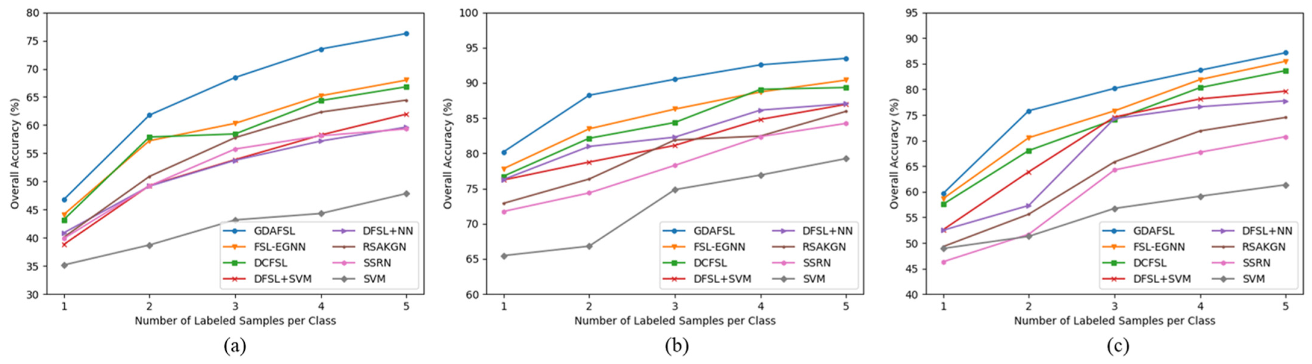
4.5. Comparision Experimental Results

To evaluate the classification performance of GDAFSL, several state-of-the-art are selected to conduct comparative experiments, including ordinary SVM, SSRN [16], RSAKGN [26], DFSL + NN [30], DFSL + SVM [30], DCFSL [42], and FSL-EGNN [41].

Table 7. Classification Results (%) of Various HSI Classification Methods on IP Dataset with 5 Labeled Samples Per Class.

Class	SVM	SSRN	RSAKGN	DFSL + NN	DFSL + SVM	DCFSL	FSL-EGNN	GDAFSL
1	27.45	92.22	96.11	96.75	96.75	95.37	98.26	99.51
2	37.90	47.19	43.93	38.65	36.38	43.26	58.11	61.25
3	24.13	40.29	57.54	42.79	38.34	57.95	56.47	63.96
4	25.04	85.20	93.30	68.10	77.16	80.60	82.95	92.03
5	54.59	69.09	76.81	71.20	73.92	72.91	76.23	79.18
6	81.61	85.25	92.92	76.18	86.25	87.96	91.26	89.31
7	26.46	100.00	100.00	100.00	97.10	99.57	100.00	100.00
8	94.59	80.24	88.38	74.84	81.82	86.26	92.91	96.19
9	12.74	100.00	100.00	100.00	75.56	99.33	100.00	100.00
10	36.85	63.69	61.50	47.98	52.22	62.44	57.60	71.42
11	59.51	33.05	50.07	57.95	59.96	62.75	67.56	72.56
12	21.55	56.09	59.55	38.21	36.56	48.72	52.01	64.93
13	71.55	97.49	99.18	97.50	98.00	99.35	96.98	97.50
14	86.02	92.56	79.31	83.44	84.63	85.40	92.70	89.10
15	29.60	62.13	67.58	62.29	74.10	66.69	72.64	87.45
16	80.59	97.83	97.23	100.00	100.00	97.61	98.17	92.95
OA (%)	47.86 ± 2.04	59.32 ± 7.76	64.44 ± 6.60	59.65 ± 0.63	61.69 ± 1.85	66.81 ± 2.37	67.99 ± 1.88	76.26 ± 0.97
AA (%)	48.13 ± 2.88	75.14 ± 5.31	78.96 ± 3.78	72.24 ± 0.42	73.05 ± 0.84	77.89 ± 0.8	80.87 ± 1.80	84.83 ± 0.73
κ × 100	41.75 ± 2.08	54.96 ± 8.09	60.43 ± 6.97	54.55 ± 0.52	56.78 ± 1.90	62.64 ± 0.86	63.71 ± 2.16	73.21 ± 1.04

,

Table 8. Classification Results (%) of Various HSI Classification Methods on UP Dataset with 5 Labeled Samples Per Class.

Class	SVM	SSRN	RSAKGN	DFSL + NN	DFSL + SVM	DCFSL	FSL-EGNN	GDAFSL
1	91.85	75.87	73.31	69.19	73.43	82.20	88.40	88.02
2	84.01	66.95	69.64	84.63	89.25	87.74	84.61	87.58
3	29.72	61.30	72.71	57.47	48.09	67.46	79.44	76.33
4	51.51	80.65	88.31	89.99	84.72	93.16	85.55	91.31
5	93.90	99.24	98.52	100.00	99.65	99.49	99.62	98.74
6	36.54	61.57	62.97	71.23	67.81	77.32	78.32	77.51
7	35.17	91.15	80.75	70.62	64.48	81.18	92.50	91.37
8	62.04	66.54	48.32	58.13	67.37	66.73	87.32	91.72
9	99.79	95.46	97.55	96.92	92.92	98.66	96.03	93.43
OA (%)	61.35 ± 7.11	70.75 ± 5.01	74.51 ± 4.56	77.75 ± 1.16	79.63 ± 1.09	83.65 ± 1.77	85.48 ± 2.47	87.14 ± 2.01
AA (%)	64.95 ± 2.99	77.64 ± 4.87	78.66 ± 5.61	77.57 ± 0.31	76.41 ± 1.39	83.77 ± 1.74	87.98 ± 2.01	88.45 ± 2.82
κ × 100	52.71 ± 7.07	63.04 ± 3.71	67.68 ± 6.27	71.11 ± 1.22	73.05 ± 1.60	78.70 ± 2.01	81.11 ± 3.19	83.18 ± 2.69

and

Table 9. Classification Results (%) of Various HSI Classification Methods on SV Dataset with 5 Labeled Samples Per Class.

Class	SVM	SSRN	RSAKGN	DFSL + NN	DFSL + SVM	DCFSL	FSL-EGNN	GDAFSL
1	92.88	78.68	95.42	95.63	73.92	99.40	97.79	98.88
2	98.30	99.89	94.18	99.09	96.85	99.76	99.93	99.53
3	80.47	69.19	65.58	94.01	96.28	91.96	90.53	97.62
4	96.83	97.90	99.23	99.54	99.11	99.55	98.70	98.87
5	89.04	93.57	91.47	90.58	80.72	92.70	94.84	93.15
6	99.79	98.94	99.91	98.47	91.63	99.52	99.78	98.86
7	90.47	95.56	99.56	99.81	97.73	98.88	99.78	99.39
8	67.42	69.43	67.51	77.74	82.33	74.57	76.75	86.83
9	96.45	90.52	96.37	91.13	94.44	99.59	99.12	99.65
10	77.64	81.44	83.98	60.98	80.96	86.42	88.34	89.02
11	57.96	91.79	90.88	95.99	93.38	96.61	97.18	99.02
12	91.73	96.15	96.87	93.13	97.94	99.93	98.83	99.38
13	83.27	95.31	99.81	99.34	95.79	99.30	99.72	98.95
14	83.99	97.46	96.02	98.06	98.87	98.85	99.10	98.40
15	51.21	71.92	77.42	77.54	71.13	75.38	78.27	85.10
16	90.32	91.09	96.16	85.05	90.57	92.22	94.84	90.61
OA (%)	79.25 ± 3.42	84.25 ± 2.91	85.96 ± 4.45	87.05 ± 0.83	86.95 ± 1.30	89.34 ± 2.19	90.39 ± 2.27	93.48 ± 0.78
AA (%)	84.23 ± 1.96	88.68 ± 3.10	90.65 ± 2.86	91.01 ± 0.66	90.08 ± 1.44	94.04 ± 1.14	94.59 ± 1.50	95.82 ± 0.47
κ × 100	77.03 ± 3.69	82.53 ± 3.16	84.48 ± 4.84	85.63 ± 0.91	85.51 ± 1.42	88.17 ± 1.53	89.32 ± 2.52	92.75 ± 0.87

report the quantitative experimental results acquired by different HSI classification methods on three HSI datasets. Compared with the machine learning methods (SVM), deep learning methods (SSRN and RSAKGN) acquired more satisfactory classification performance on all three target datasets. We consider that the higher classification accuracy is mainly caused by the sufficient capability of deep models to extract discriminative semantic features. Compared with deep learning methods (SSRN and RSAKGN), FSL methods (DFSL + NN, DFSL + SVM, DCFSL, and FSL-EGNN) and our GDAFSL achieve more excellent classification performances with limited training samples, which demonstrates the effectiveness of FSL methods for learning transfer knowledge.

For the abovementioned FSL methods, the proposed GDAFSL achieves the best classification performance. The OAs of GDAFSL on IP, UP, and SV datasets are 76.26%, 87.14%, and 93.48%, respectively. Compared with those FSL methods without domain adaptation (DFSL + NN and DFSL + SVM), the domain adaptation FSL methods (DCFSL and GDAFSL) generate better classification performance. Due to adding GDAN to explore domain similarities, GDAFSL achieves more satisfactory classification results. The OAs of GDAFSL are 9.45%, 3.49%, and 4.14% higher than that of DCFSL on IP, UP, and SV datasets, which demonstrates the effectiveness of GDAN. When compared with FSL-EGNN which achieves the second-best classification performance, GDAFSL achieves higher classification performance by virtue of the specifically designed domain adaptation module. The OAs of GDAFSL are 8.27%, 1.66%, and 3.09% higher than that of FSL-EGNN on IP, UP, and SV data sets, which demonstrated the superiority of our proposed GDAFSL method.

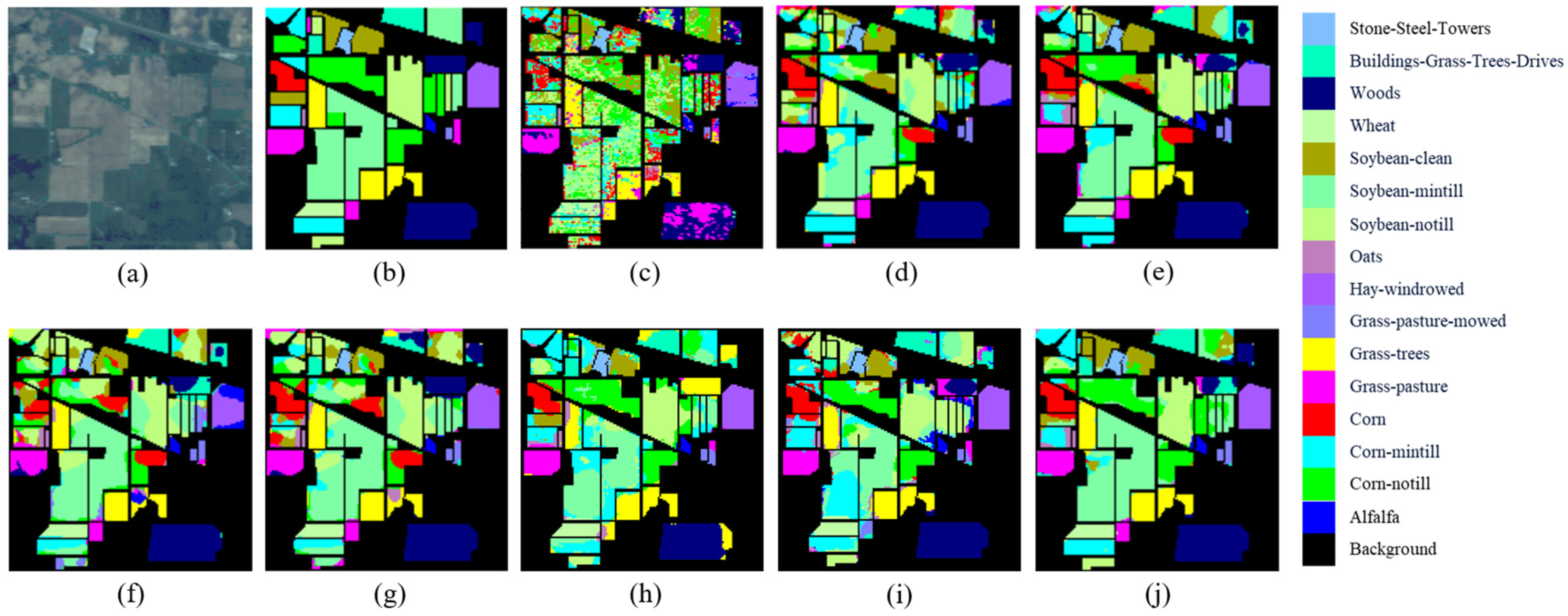
It is worth noting that the GDAFSL achieves a more significant improvement of classification performance on the IP dataset than on the UP and SV dataset. This is mainly because the GDAFSL significantly improves the accuracy of those hardly classified classes which are easily misclassified by other methods and have extremely lower classification accuracy, such as class 3 (Corn-mintill), class 10 (Soybean-notill), class 11 (Soybean-mintill), and class 15 (Buildings-Grass-Trees-Drives).

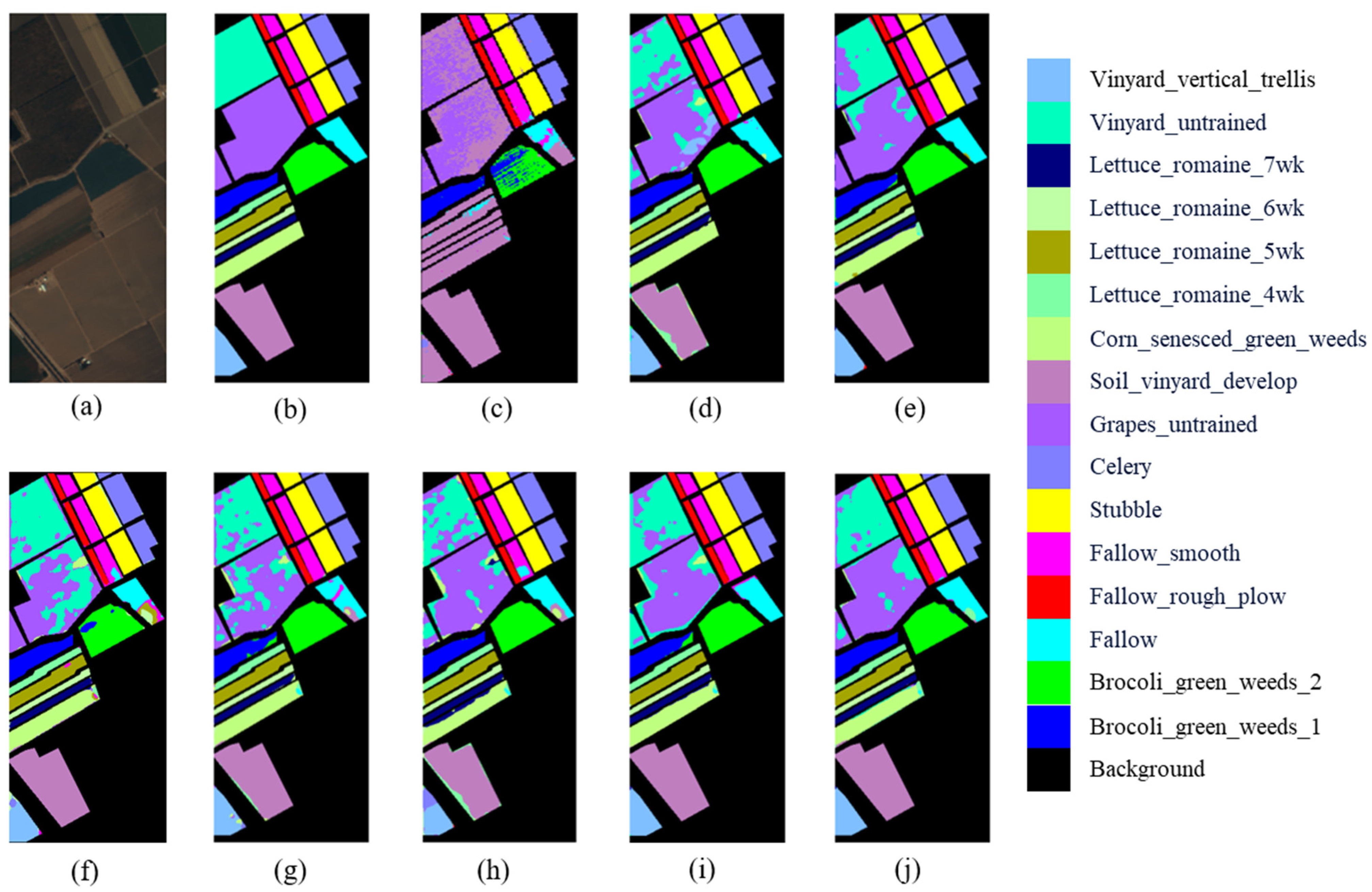
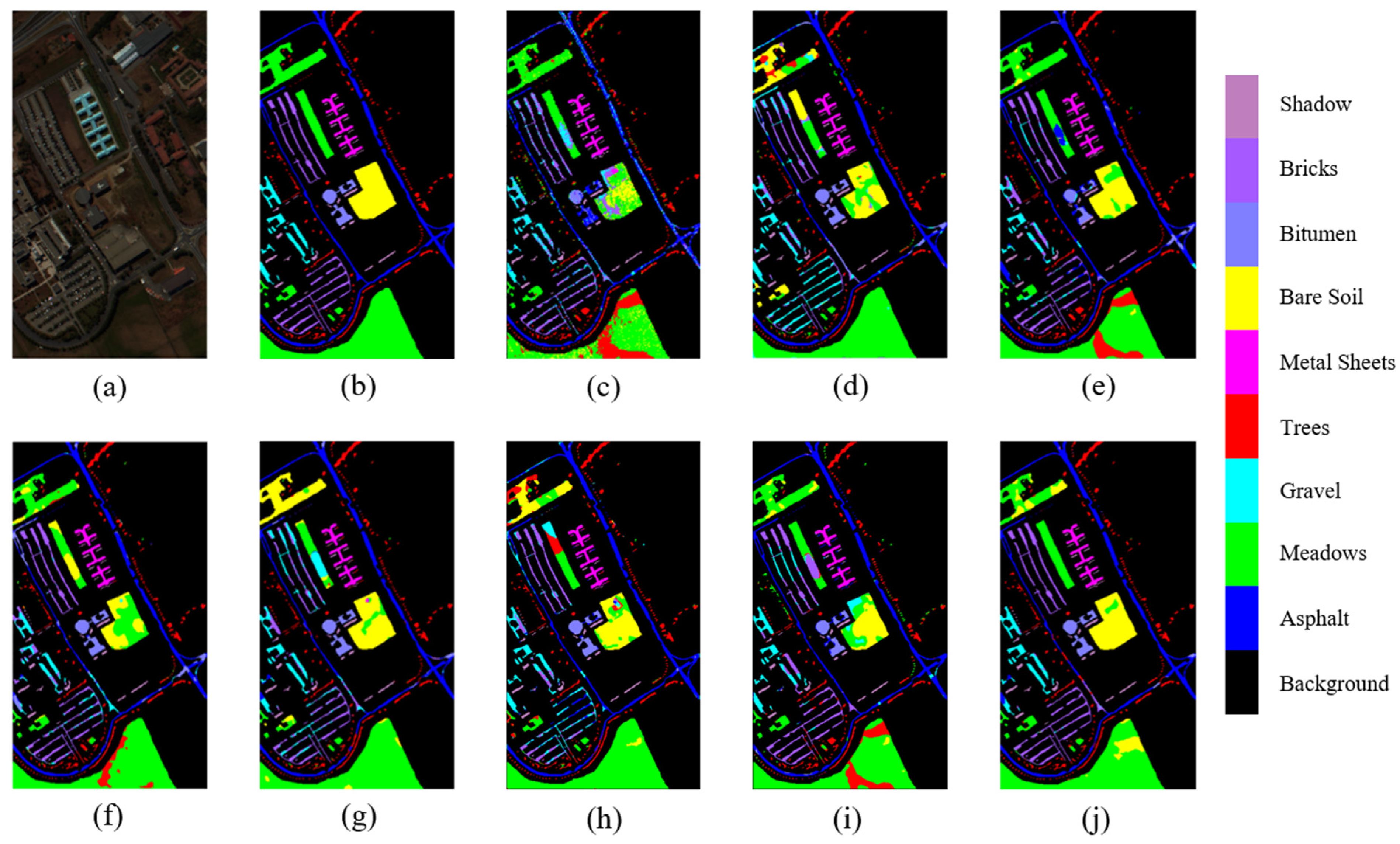
To further intuitively evaluate the classification performance of GDAFSL, classification maps of three target datasets generated by various HSI classification methods are presented in Figure 14, Figure 15 and Figure 16. GDAFSL can generate more precise and consistent classification maps which have fewer misclassification pixels. Compared with reference methods, GDAFSL can not only significantly increase the intra-class consistency in the homogeneous region, but also decrease the inter-class differences in border areas. These classification maps also demonstrate the superiority of GDAFSL in a more intuitive view.

5. Discussion

Extensive experiments with 1–5 shot labeled samples per class are conducted on three target datasets to verify the impact of various labeled sample sizes per class in ${\mathit{D}}_T^f$. The experimental results are presented in Figure 17. It is obvious that the OAs of all classification methods generally raise with the increases in labeled sample size and the proposed GDAFSL can continuously outperform other HSI classification methods on three target datasets. It is worth noting that even if the labeled samples are extremely insufficient, such as only 1 or 2 shots per class, our GDAFSL still has a competitive classification performance, which can further demonstrate the robustness and effectiveness of GDAFSL.

To intuitively evaluate the complexity of GDAFSL, the training and testing times, and the number of parameters are reported in

Table 10. Training Time, Testing Time, and Parameters of Different HSI Classification Methods on Three Target Datasets.

Dataset		SVM	SSRN	RSAKGN	DFSL + NN	DFSL + SVM	DCFSL	FSL-EGNN	GDAFSL
IP	Training (s)	0.24	31.58	21.37	703.82	470.45	1255.45	2487.56	1564.63
	Testing (s)	0.41	4.91	2.71	1.28	4.71	1.39	12.89	1.35
	Parameters	-	735,884	67,504	34,920	34,920	4,268,994	68,733	108,061
UP	Training (s)	0.31	39.63	27.09	436.71	648.47	1251.64	2028.88	1351.49
	Testing (s)	0.65	6.38	4.31	5.07	5.10	5.22	42.37	5.26
	Parameters	-	396,993	74,281	34,920	34,920	4,259,294	68,733	98,361
SV	Training (s)	0.25	27.91	22.51	951.37	510.72	1287.21	2837.77	2224.01
	Testing (s)	1.74	8.08	6.71	6.59	14.23	7.44	78.35	7.58
	Parameters	-	749,996	67,888	34,920	34,920	4,269,394	68,733	108,461

. Compared with ordinary deep learning methods, FSL methods generally require longer training time to conduct a time-consuming transfer learning process. As shown in Table 10, owning to continuously update the graph constructions, those graph-based methods, FSL-EGNN and GDAFSL, are more time-consuming than other FSL methods. The FSL-EGNN, which utilizes graph construction to generate predicted labels, achieves the longest training and testing times. Different from FSL-EGNN, the graph construction in GDAFSL is only utilized in the training stage to perform the domain adaptation learning process. Therefore, GDAFSL can achieve fast and accurate classification in the testing stage.

6. Conclusions

In this article, a novel cross-domain FSL method called GDAFSL is introduced to tackle the domain shift problem in cross-domain few-shot HSI classification. The proposed method focuses on learning a domain invariant feature representation space and achieving cross-domain few-shot HSI classification by exploring the correlations between samples of different domains. Specifically designed feature extractor DRHAN, which can effectively model the spatial interactions in different scales pixel neighborhoods, is proposed to extract discriminative semantic features. Then, by combining graph construction with domain adversarial strategy, a graph-based domain adaptation network, which can dynamically update graph construction to fully explore domain correlations, is designed to overcome domain shift. In addition, to properly model domain correlations in graph construction, a novel similarity measurement method is proposed to perform feature aggregation on samples with non-Euclidean structural characteristics. By performing such domain adaptation FSL with a meta-learning paradigm, a discriminative domain-invariant metric space is learned to execute a few-shot HSI classification. Comprehensive experimental results conducted on three public HSI data sets demonstrate the effectiveness and superiority of GDAFSL.

References

1. Ghamisi, P.; Mura, M.D.; Benediktsson, J.A. A survey on spectral–spatial classification techniques based on attribute profiles. IEEE Trans. Geosci. Remote Sens. 2015, 53, 2335–2353. [Google Scholar] [CrossRef]
2. Bioucas-Dias, J.; Plaza, A.; Camps-Valls, G.; Scheunders, P.; Nasrabadi, N.; Chanussot, J. Hyperspectral remote sensing data analysis and future challenges. IEEE Geosci. Remote Sens. Mag. 2013, 1, 6–36. [Google Scholar] [CrossRef] [Green Version]
3. Liang, L.; Di, L.; Zhang, L.; Deng, M.; Qin, Z.; Zhao, S.; Lin, H. Estimation of crop LAI using hyperspectral vegetation indices and a hybrid inversion method. Remote Sens. Environ. 2015, 165, 123–134. [Google Scholar] [CrossRef]
4. Yang, X.; Yu, Y. Estimating soil salinity under various moisture conditions: An experimental study. IEEE Trans. Geosci. Remote Sens. 2017, 55, 2525–2533. [Google Scholar] [CrossRef]
5. Chen, Y.; Lin, Z.; Zhao, X.; Wang, G.; Gu, Y. Deep learning-based classification of hyperspectral data. IEEE J. Sel. Top. Appl. Earth Observ. Remote Sens. 2014, 7, 2094–2107. [Google Scholar] [CrossRef]
6. Li, T.; Zhang, J.; Zhang, T. Classification of hyperspectral image based on deep belief networks. In Proceedings of the IEEE International Conference on Image Process (ICIP), Parise, France, 27–39 October 2014; pp. 5132–5136. [Google Scholar]
7. Chen, Y.; Jiang, H.; Li, C.; Jia, X.; Ghamisi, P. Deep feature extraction and classification of hyperspectral images based on convolutional neural networks. IEEE Trans. Geosci. Remote Sens. 2016, 54, 6232–6251. [Google Scholar] [CrossRef] [Green Version]
8. Liu, B.; Yu, X.; Zhang, P.; Yu, A.; Fu, Q.; Wei, X. Supervised deep feature extraction for hyperspectral image classification. IEEE Trans. Geosci. Remote Sens. 2018, 56, 1909–1921. [Google Scholar] [CrossRef]
9. Zhao, W.; Du, S. Spectral–spatial feature extraction for hyperspectral image classification: A dimension reduction and deep learning approach. IEEE Trans. Geosci. Remote Sens. 2016, 54, 4544–4554. [Google Scholar] [CrossRef]
10. Cao, X.; Zhou, F.; Xu, L.; Meng, D.; Xu, Z.; Paisley, J. Hyperspectral image classification with Markov random fields and a convolutional neural network. IEEE Trans. Image Process. 2018, 27, 2354–2367. [Google Scholar] [CrossRef] [Green Version]
11. Li, Y.; Zhang, H.; Shen, Q. Spectral–spatial classification of hyperspectral imagery with 3D convolutional neural network. Remote Sens. 2017, 9, 67. [Google Scholar] [CrossRef] [Green Version]
12. Ben Hamida, A.; Benoit, A.; Lambert, P.; Ben Amar, C. 3-D deep learning approach for remote sensing image classification. IEEE Trans. Geosci. Remote Sens. 2018, 56, 4420–4434. [Google Scholar] [CrossRef] [Green Version]
13. Yang, X.; Ye, Y.; Li, X.; Lau, R.Y.K.; Zhang, X.; Huang, X. Hyperspectral image classification with deep learning models. IEEE Trans. Geosci. Remote Sens. 2018, 56, 5408–5423. [Google Scholar] [CrossRef]
14. He, K.; Zhang, X.; Ren, S.; Sun, J. Deep residual learning for image recognition. In Proceedings of the IEEE Conference on Computer Vision and Pattern Recognition (CVPR), Seattle, WA, USA, 27–30 June 2016; pp. 770–778. [Google Scholar] [CrossRef] [Green Version]
15. Paoletti, M.E.; Haut, J.M.; Fernandez-Beltran, R.; Plaza, J.; Plaza, A.J.; Pla, F. Deep pyramidal residual networks for spectral-spatial hyperspectral image classification. IEEE Trans. Geosci. Remote Sens. 2019, 57, 740–754. [Google Scholar] [CrossRef]
16. Zhong, Z.; Li, J.; Luo, Z.; Chapman, M. Spectral–spatial residual network for hyperspectral image classification: A 3-D deep learning framework. IEEE Trans. Geosci. Remote Sens. 2018, 56, 847–858. [Google Scholar] [CrossRef]
17. Song, W.; Li, S.; Fang, L.; Lu, T. Hyperspectral image classification with deep feature fusion network. IEEE Trans. Geosci. Remote Sens. 2018, 56, 3173–3184. [Google Scholar] [CrossRef]
18. Wang, W.; Dou, S.; Jiang, Z.; Sun, L. A fast dense spectral-spatial convolution network framework for hyperspectral images classification. Remote Sens. 2018, 10, 1068. [Google Scholar] [CrossRef] [Green Version]
19. Li, W.; Wu, G.; Zhang, F.; Du, Q. Hyperspectral image classification using deep pixel-pair features. IEEE Trans. Geosci. Remote Sens. 2017, 55, 844–853. [Google Scholar] [CrossRef]
20. Zheng, C.; Wang, N.; Cui, J. Hyperspectral image classification with small training sample size using superpixel-guided training sample enlargement. IEEE Trans. Geosci. Remote Sens. 2019, 57, 7307–7316. [Google Scholar] [CrossRef]
21. Dong, S.; Quan, Y.; Feng, W.; Dauphin, G.; Gao, L.; Xing, M. A pixel cluster CNN and spectral-spatial fusion algorithm for hyperspectral image classification with small-size training samples. IEEE J. Sel. Top. Appl. Earth Observ. 2021, 14, 4101–4114. [Google Scholar] [CrossRef]
22. Aydemir, M.S.; Bilgin, G. Semisupervised hyperspectral image classification using small sample sizes. IEEE Geosci. Remote Sens. Lett. 2017, 14, 621–625. [Google Scholar] [CrossRef]
23. Sun, H.; Zheng, X.; Lu, X.; Wu, S. Spectral–spatial attention network for hyperspectral image classification. IEEE Trans. Geosci. Remote Sens. 2020, 58, 3232–3245. [Google Scholar] [CrossRef]
24. Zhu, M.; Jiao, L.; Liu, F.; Yang, S.; Wang, J. Residual spectral–spatial attention network for hyperspectral image classification. IEEE Trans. Geosci. Remote Sens. 2021, 59, 449–462. [Google Scholar] [CrossRef]
25. Zhong, Z.; Li, Y.; Ma, L.; Li, L.; Zheng, W. Spectral-Spatial transformer network for hyperspectral image classification: A factorized architecture search framework. IEEE Trans. Geosci. Remote Sens. 2022, 60, 5514715. [Google Scholar] [CrossRef]
26. Xu, Y.; Zhang, Y.; Yu, C.; Ji, C.; Yue, T.; Li, H. Residual spatial attention kernel generation network for hyperspectral image classification with small sample size. IEEE Trans. Geosci. Remote Sens. 2022, 60, 5529714. [Google Scholar] [CrossRef]
27. Chen, W.; Liu, Y.; Kira, Z.; Wang, Y.; Huang, J. A closer look at few-shot classification. arXiv 2019, arXiv:1904.04232. [Google Scholar]
28. Wang, Y.; Yao, Q.; Kwok, J.; Ni, L. Generalizing from a few examples: A survey on few-shot learning. ACM Comput. Surv. 2020, 53, 63. [Google Scholar] [CrossRef]
29. Snell, J.; Swersky, K.; Zemel, R. Prototypical networks for few-shot learning. arXiv 2017, arXiv:1703.05175. [Google Scholar]
30. Liu, B.; Yu, X.; Yu, A.; Zhang, P.; Wan, G.; Wang, R. Deep few-shot learning for hyperspectral image classification. IEEE Trans. Geosci. Remote Sens. 2019, 57, 2290–2304. [Google Scholar] [CrossRef]
31. Gao, K.; Liu, B.; Yu, X.; Qin, J.; Zhang, P.; Tan, X. Deep relation network for hyperspectral image few-shot classification. Remote Sens. 2020, 12, 923. [Google Scholar] [CrossRef] [Green Version]
32. Tang, H.; Huang, Z.; Li, Y.; Zhang, L.; Xie, W. A multiscale spatial–spectral prototypical network for hyperspectral image few-shot classification. IEEE Geosci. Remote Sens. Lett. 2022, 19, 6011205. [Google Scholar] [CrossRef]
33. Liang, X.; Zhang, Y.; Zhang, J. Attention multisource fusion-based deep few-shot learning for hyperspectral image classification. IEEE J. Sel. Topics Appl. Earth Observ. 2021, 14, 8773–8788. [Google Scholar] [CrossRef]
34. Xi, B.; Li, J.; Li, Y.; Song, R.; Shi, Y.; Liu, S.; Du, Q. Deep prototypical networks with hybrid residual attention for hyperspectral image classification. IEEE J. Sel. Topics Appl. Earth Observ. 2020, 13, 3683–3700. [Google Scholar] [CrossRef]
35. Wang, Y.; Liu, M.; Yang, Y.; Li, Z.; Du, Q.; Chen, Y.; Li, F.; Yang, H. Heterogeneous Few-shot learning for hyperspectral image classification. IEEE Geosci. Remote Sens. Lett. 2021, 19, 5510405. [Google Scholar] [CrossRef]
36. Liu, S.; Shi, Q.; Zhang, L. Few-shot hyperspectral image classification with unknown classes using multitask deep learning. IEEE Trans. Geosci. Remote Sens. 2021, 59, 5085–5102. [Google Scholar] [CrossRef]
37. Hong, D.; Gao, L.; Yao, J.; Zhang, B.; Plaza, A.; Chanussot, J. Graph Convolutional Networks for Hyperspectral Image Classification. IEEE Trans. Geosci. Remote Sens. 2021, 59, 5966–5978. [Google Scholar] [CrossRef]
38. Wan, S.; Pan, S.; Zhong, P.; Chang, X.; Yang, J.; Gong, C. Dual Interactive Graph Convolutional Networks for Hyperspectral Image Classification. IEEE Trans. Geosci. Remote Sens. 2022, 60, 5510214. [Google Scholar] [CrossRef]
39. Bai, J.; Ding, B.; Xiao, Z.; Jiao, L.; Chen, H.; Regan, A.C. Hyperspectral Image Classification Based on Deep Attention Graph Convolutional Network. IEEE Trans. Geosci. Remote Sens. 2022, 60, 5504316. [Google Scholar] [CrossRef]
40. Wan, S.; Gong, C.; Zhong, P.; Pan, S.; Li, G.; Yang, J. Hyperspectral image classification with context-aware dynamic graph convolutional network. IEEE Trans. Geosci. Remote Sens. 2021, 59, 597–612. [Google Scholar] [CrossRef]
41. Zuo, X.; Yu, X.; Liu, B.; Zhang, P.; Tan, X. FSL-EGNN: Edge-labeling graph neural network for hyperspectral image few-shot classification. IEEE Trans. Geosci. Remote Sens. 2022, 60, 5526518. [Google Scholar] [CrossRef]
42. Li, Z.; Liu, M.; Chen, Y.; Xu, Y.; Li, W.; Du, Q. Deep cross-domain few-shot learning for hyperspectral image classification. IEEE Trans. Geosci. Remote Sens. 2022, 60, 5501618. [Google Scholar] [CrossRef]
43. Bai, J.; Huang, S.; Xiao, Z.; Li, X.; Zhu, Y.; Regan, A.C.; Jiao, L. Few-shot hyperspectral image classification based on adaptive subspaces and feature transformation. IEEE Trans. Geosci. Remote Sens. 2022, 60, 5523917. [Google Scholar] [CrossRef]
44. Woo, S.; Park, J.; Lee, J.; Kweon, I.S. CBAM: Convolutional block attention module. In Proceedings of the European Conference on Computer Vision (ECCV), Munich, Germany, 8–14 September 2018; pp. 3–19. [Google Scholar] [CrossRef] [Green Version]
45. Li, D.; Hu, J.; Wang, C.; Li, X.; She, Q.; Zhu, L.; Zhang, T.; Chen, Q. Involution: Inverting the inherence of convolution for visual Recognition. arXiv 2021, arXiv:2103.06255. [Google Scholar]
46. He, X.; Chen, Y.; Ghamisi, P. Heterogeneous transfer learning for hyperspectral image classification based on convolutional neural network. IEEE Trans. Geosci. Remote Sens. 2020, 58, 3246–3263. [Google Scholar] [CrossRef]
47. Long, M.; Cao, Z.; Wang, J.; Jordan, M.I. Conditional adversarial domain adaptation. In Proceedings of the Conference on Neural Information Processing Systems (NIPS), Montreal, QC, Canada, 2–8 October 2018; pp. 1640–1650. [Google Scholar]
Figure 1. Framework of the proposed GDAFSL.
Remotesensing 15 01125 g001
Figure 2. Structure of the GAMM used in DRHAN.
Remotesensing 15 01125 g002
Figure 3. Structure of the LAEM used in DRHAN.
Remotesensing 15 01125 g003
Figure 4. Flowchart of the local attention mechanism used in LAEM.
Remotesensing 15 01125 g004
Figure 5. The architecture of feature extractor DRHAN. For convenience, batch normalization and reflect linear units following convolutional layers are not presented.
Remotesensing 15 01125 g005
Figure 6. Structure of the proposed GDAN.
Remotesensing 15 01125 g006
Figure 7. Illustration of GCM used in GDAN. The nodes with different colors denote samples of different domains. Lines of different thicknesses represent different sizes and values of edge weights.
Remotesensing 15 01125 g007
Figure 8. Structure of GUM used in GDAN.
Remotesensing 15 01125 g008
Figure 9. OAs obtained by GDAFSL with different initial learning rates on three target datasets.
Remotesensing 15 01125 g009
Figure 10. OAs obtained by GDAFSL with different numbers of epochs on three target datasets.
Remotesensing 15 01125 g010
Figure 11. OAs obtained by GDAFSL with different size of task. (a) The number of support samples. (b) The number of query samples.
Remotesensing 15 01125 g011
Figure 12. OAs obtained by GDAFSL with various neighborhood sizes on three HSI datasets.
Remotesensing 15 01125 g012
Figure 13. OAs obtained by GDFSL with various numbers of GUM on three HSI datasets.
Remotesensing 15 01125 g013
Figure 14. Classification maps of various HSI classification methods on IP dataset. (a) False-Color maps. (b) Ground Truth. (cj) SVM, SSRN, RSAKGN, DFSL + NN, DFSL + SVM, DCFSL, FSL-EGNN, and GDAFSL, respectively.
Remotesensing 15 01125 g014
Figure 15. Classification maps of various HSI classification methods on the SV dataset. (a) False-Color maps. (b) Ground Truth. (cj) SVM, SSRN, RSAKGN, DFSL + NN, DFSL + SVM, DCFSL, FSL-EGNN, and GDAFSL, respectively.
Remotesensing 15 01125 g015
Figure 16. Classification maps of various HSI classification methods on the UP dataset. (a) False-Color maps. (b) Ground Truth. (cj) SVM, SSRN, RSAKGN, DFSL+NN, DFSL+SVM, DCFSL, FSL-EGNN, and GDAFSL, respectively.
Remotesensing 15 01125 g016
Figure 17. OA (%) of eight HSI classification methods with various labeled sample sizes on three target datasets. (a) IP. (b) UP. (c) SV.
Remotesensing 15 01125 g017