Physical Mechanism and Parameterization for Correcting Radar Wave Velocity in Yellow River Ice with Air Temperature and Ice Thickness

Abstract

Unfrozen free and non-free water between ice crystals in flat and hummock ice in the Yellow River exists as water films with varying contents based on ice temperature. These contents can affect the radar wave velocity of the ice despite its theoretical dependence on the crystal structure and ice body components. The unfrozen water content in ice depends on the ice temperature, which is controlled by the air temperature, solar radiation, and ice thickness. Winter air temperature and radar-detected ice thickness data observed at the Shisifenzi bend in the Yellow River from 2020 to 2021 were analyzed. The unfrozen water content in the ice was the primary factor influencing the accuracy of flat ice thickness detection. The heat flux at the ice–water interface in the Yellow River was determined. The evolution of ice thickness and temperature were simulated using a one-dimensional (1D) ice thermodynamic model forced by the local weather station data (i.e., air temperature, solar radiation, wind speed, and cloud cover). On this basis, the measured ice thickness data of 13 drill holes were combined to calculate 1251 thermodynamically simulated ice thicknesses consistent with the ice thickness detection time of the radar; therefore, statistical relationships regarding the influence of air temperature and the combined action of air temperature and ice thickness on the radar wave velocity in granular and columnar ice during air temperature increases and decreases were determined. Finally, the statistical relationship between the combined influence of air temperature and ice thickness on radar wave velocity was selected as a parameterization scheme to dynamically correct the radar wave velocity of flat ice. To enhance the radar detection accuracy for flat ice thickness, the radar wave velocity of ice was parameterized as a function. Given the presence of unfrozen frazil ice and accumulated broken ice blocks in the Yellow River, radar is suggested to detect the thickness of different types of ice in future research.

1. Introduction

Ground-penetrating radar (GPR), a type of nondestructive detection equipment, has been extensively applied to detect soil water content [1] and density [2] and the water depth of rivers and ponds [3]. GPR has been applied for analyses in the cryosphere, e.g., glacier ice, sea ice, lake ice, river ice, reservoir ice, cave ice, snow, and frozen soil. The dielectric permittivity and wave propagation velocity of radar, abbreviated as radar wave velocity, are the main parameters of radar detection and are affected by the physical properties of ice, snow, soil, or meteorological conditions. Unfrozen water in glacier ice within 0–5% causes the radar wave velocity to decelerate to within 0.168–0.138 m ns⁻¹ [4]. For Antarctic sea ice thickness detection, the dielectric permittivity was set between 2.5 and 8.0 [5], because it is potentially more sensitive to the brine volume fraction and is influenced by temperature and microstructural features, including pore volume [6]. For snow detection, liquid water contents are inputted to calculate the dielectric permittivity, which has been developed into different mixed-model approaches [7]. For the detection of different permafrost layers using different radar beams, water content in the active layers was found to reach up to 70% [8]. Additionally, GPR technology has developed rapidly for ice thickness measurements of reservoirs, lakes, and rivers.

In the 1980s, the ice thickness evolution of an Alaskan lake and two rivers were detected using short-pulse radar with 600 and 900 MHz antennae mounted inside of helicopters [9,10]. In December 2008, Li et al. [11] detected the ice thickness at 25 points in a reservoir in northeastern China using GPR with 600 MHz antennae and analyzed the effects of ice physical properties on detection precision through measured ice crystals, bubble content, and ice density. Liu et al. [12,13,14] developed new GPR system and proposed an envelope spectrum to estimate the dielectric permittivity from 2011 to 2014. In March 2012, Gusmeroli and Grosse [15] surveyed ice–snow thickness evolution of three thermokarst lakes in Alaska using GPR with a 1 GHz antenna and found that the radar reflection intensities from wet snow–ice interfaces were at least twice those from dry snow–ice interfaces. In January 2014, Zhang et al. [16] detected the ice thickness of transverse and longitudinal river sections at the Toudaoguai Hydrological Station in the Yellow River with radar antennae of 200, 400, 900, and 1500 MHz and determined that radar wave velocity gradually declines over time when entering the thawing period. The radar wave velocity decreased with an increase in unfrozen water content, but the quantification of this decrease was not reported. In March 2014, Kämäri et al. [17] measured the river ice thickness of 45 cross-sections with an 800 MHz antenna and discovered a significant difference in ice thickness in a meandering river, with a maximum difference of 32 cm between cross-sections. During 2015 to 2017, Fu et al. [18] developed a double-frequency GPR with 100 and 1500 MHz, which has been applied to synchronously measure water depth and ice thickness evolution in the Heilongjiang River, Yellow River, and Wanjiazhai Reservoir. Bai et al. [19] employed GPR mounted on an unmanned aerial vehicle (UAV) to measure ice thickness in the Songhua River, which is more economical and faster than the helicopter mounting method. These GPR observations are focused on the stable ice period and lack continuous monitoring throughout ice growth and decay. The previous studies focused on the application of GPR at macroscopic or large scale in ice thickness measurement. However, this paper tries to make some efforts to improve the accuracy of GPR measurement of ice thickness at the microcosmic or small scale for engineering purposes. In fact, unfrozen water content in ice affects dielectric permittivity. The relationships between dielectric permittivity and unfrozen water content and relationships between unfrozen water content and air/ice temperature are foundational. Murray et al. [20,21] provide a potential remote technique for assessing water content based on mixture models. It is difficult to measure unfrozen water content in ice samples directly.

We developed a hanging GPR set (H–GPR–S) that can continuously obtain ice thickness data at 1 h intervals from fixed positions and video images of the ice surface. The hanging radar has fixed altitudes relative to the river bank, but it is variable relative to the ice surface with the water surface variation. In the ice season of 2019–2020, the growth and decay of the ice in the Shisifenzi bend of Yellow River was detected using the H–GPR–S. The ice thickness measured by artificial drilling three times in the growing stages could have shown the feasibility of H–GPR–S but did not serve as support for analyzing the effects of the physical properties of ice on detection precision. Therefore, ice thickness was measured every 3–5 days, 13 times in total, by drilling holes in the winter of 2020–2021. However, compared with the measured ice thickness values, there were many errors in the ice thickness detection via H–GPR–S during ice melting, possibly because the dielectric permittivity was always set to 3.2 in our H–GPR–S analysis and the radar wave velocity was also always 16.770 cm ns⁻¹. The radar wave velocity decelerated because of the unfrozen water in ice and may have accelerated because of the unevenly distributed sediments within the Yellow River ice. As previously reported, the dielectric permittivity of Yellow River ice is within 2.5–4.5, which is a comprehensive embodiment of unfrozen water and sediment content [22]. Therefore, to improve radar precision in ice thickness detection, it is necessary to take into account the dynamic correction method of the radar wave velocity. Our study mainly focused on the following components:

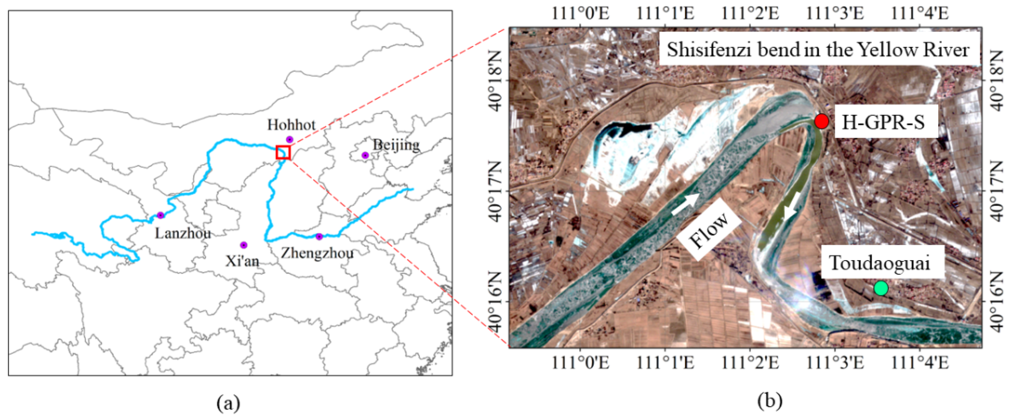
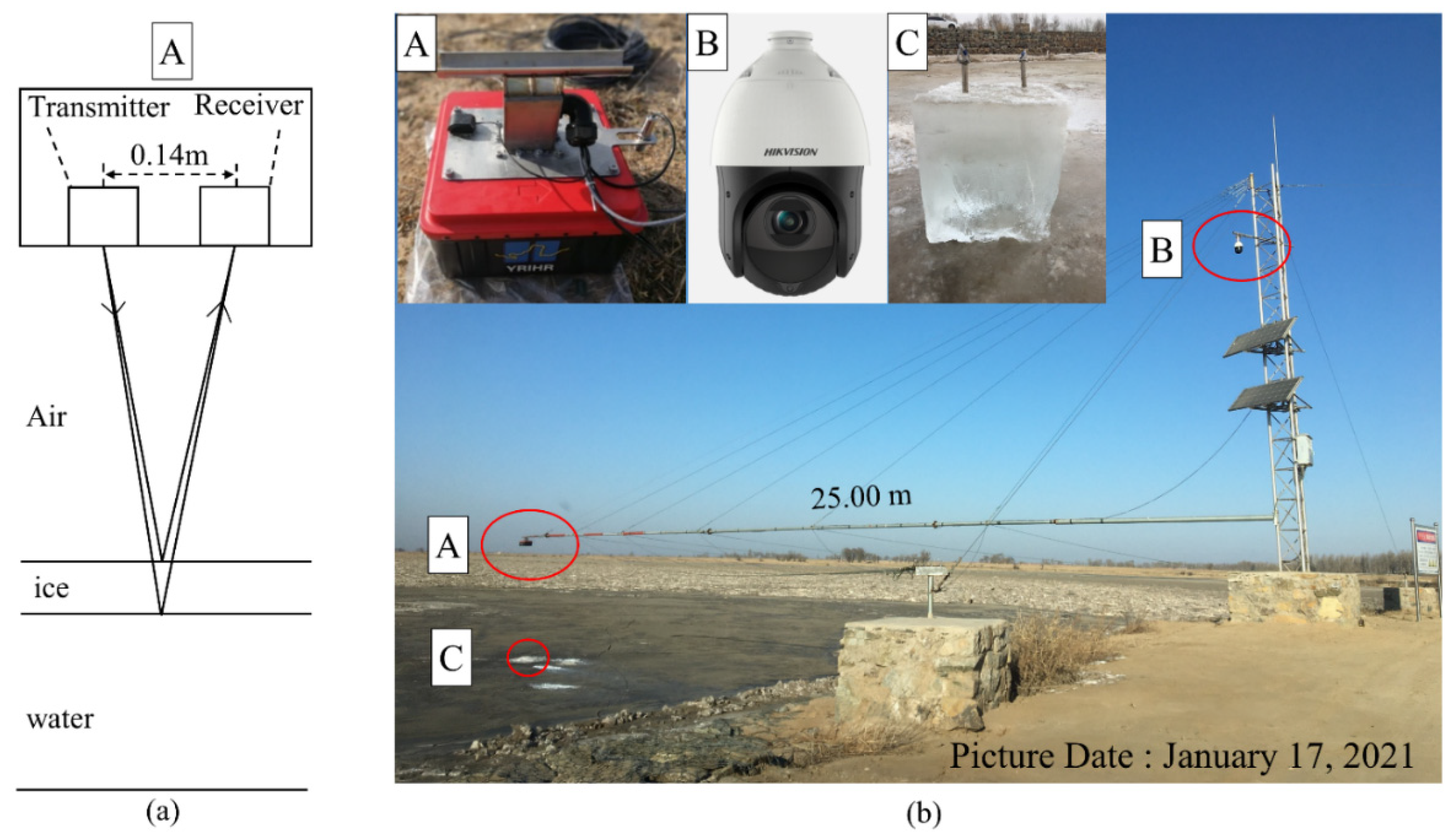
• Ice thicknesses via radar detection and measured by drilling holes were collected. Ice temperature profiles under the radar were measured. Meteorological data of the entire ice season from nearby Toudaoguai Hydrological Station were gathered. Ice density, sediment content, and crystal structure of the ice sample were tested in the Toudaoguai Hydrological Station;
• The measured ice physical data were combined to analyze the tread of the radar wave velocity or dielectric permittivity in granular and columnar ice within the ice sample;
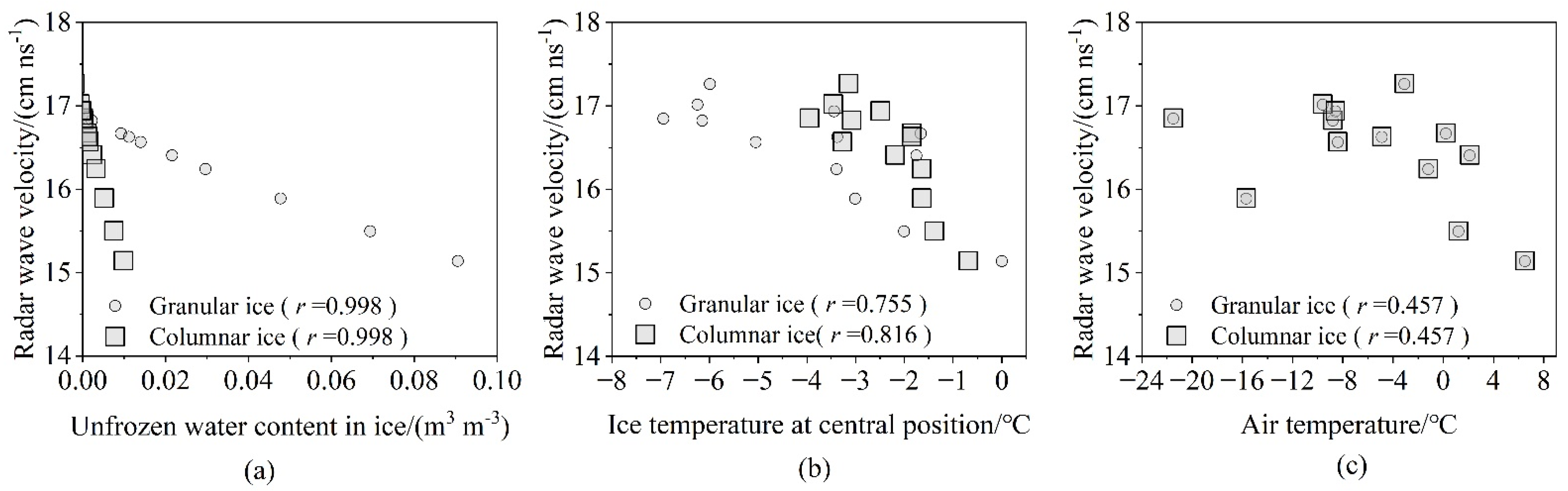
• Based on the sequence of 13 measured ice thicknesses, we sought to determine the physical logical relationship. It shows that the radar wave velocity or dielectric permittivity was controlled by the unfrozen water content in the ice. The unfrozen water content was dominated by the ice temperature, and the ice temperature was influenced by air temperature, radiation, and ice thickness;
• One parameterization scheme for dynamically correcting the radar wave velocity with air temperature and ice thickness was set up and improved the radar detection accuracy of ice thickness. The theoretical mechanism and statistical analyses results are also provided based on the previous literature;
• A method for developing a parameterization scheme for more complicated ice conditions, for example, frazil ice on the bottom of the ice cover and accumulated broken ice blocks in ice jams, was proposed as a correction to the method. A complete theoretical basis for high-precision GPR detection of the thickness of different types of ice in the Yellow River will be developed in the future.

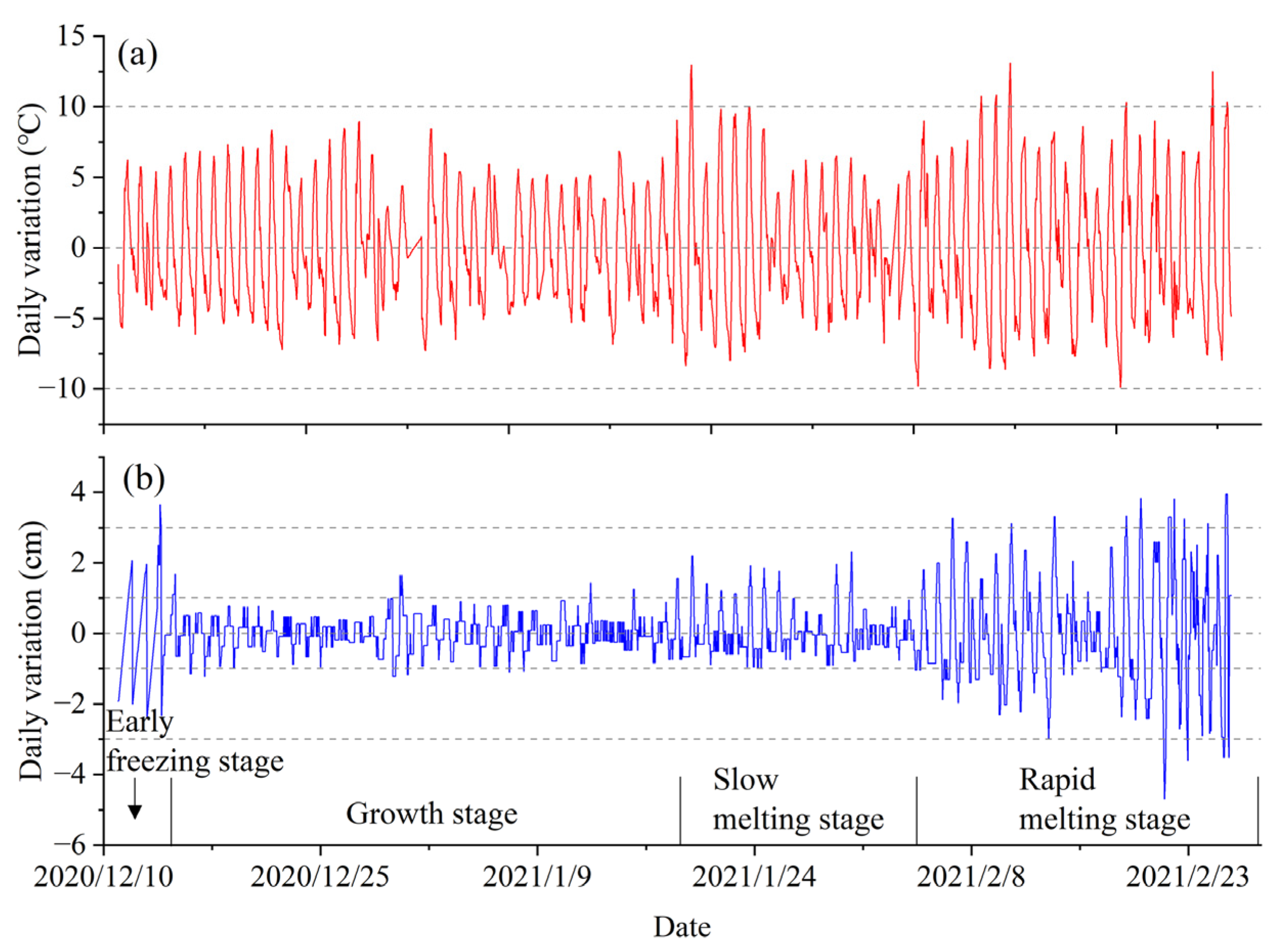
2. Hanging Ground-Penetrating Radar Set and the Characteristics of Air Temperature and Ice Thickness in Winter

H–GPR–S was installed at an iron tower in the concave bank of the Shisifenzi bend (111°2′45″ E, 40°17′43″ N) of the Yellow River mainstream (Figure 1a). The Toudaoguai Hydrological Station is 3,100 m away from the installation site of the H–GPR–S (Figure 1b). The IGPR-50 radar (A in Figure 2b) and video camera (B in Figure 2b) were the main sensors in the H–GPR–S, which detected the ice thickness at a fixed position and recorded video of the ice surface in the bend each hour, respectively. The radar was fixed at the end of a horizontal strut 25.00 m in length. Its center and sample frequencies were 400 MHz and 14.62 GHz, respectively. The distance between the transmitter antenna and receiver antenna was 0.14 m (Figure 2a) and the designed maximum detectable ice thickness was 5.00 m. The distance between the IGPR-50 and ice surface varied with water level between 3.25 m and 5.40 m in the winter of 2020–2021 (Figure 2a). The video camera had visible and infrared night vision capabilities, and its maximum video resolution was 1920 × 1080 pixels. Moreover, the video camera view was set to face downstream of the Shisifenzi bend to record the ice situation on the river surface automatically once per hour.

Figure 3 shows a typical GPR profile obtained via IGPR-50. The layer tracking algorithm [19] was used to track the radar–air interface, ice–air interface and ice–water interface automatically. The ice thickness was calculated by Equation (1).

$$H_i=v_i\Delta t=v_i\left(t2-t1\right) ,$$

(1)

where $H_i$ is the ice thickness detected by IGPR-50, cm; $v_i$ is the radar wave velocity in ice, cm ns⁻¹; $\Delta t$ is the two-way time in ice cover, ns; $t1$ and $t2$ are the two-way time from the radar–air interface to the ice–air interface and the ice–water interface, respectively, ns.

An ice sample beneath the IGPR-50 radar was removed using a chain saw on 10 January 2021, (C in Figure 2b) and the ice temperature was measured with a thermometer under the IGPR-50 radar. Then, the crystal structure of the ice sample was observed with a universal stage [22] at Toudaoguai Hydrological Station (green point in Figure 1b). The ice density and sediment content were also measured via the volume weight method.

The air temperatures and some special events in the winter of 2020–2021 are shown in Figure 4a. From 11 December 2020, to 26 February 2021, the ice thickness (black solid line in Figure 4b) detected by the IGPR-50 radar was recorded once per hour at a resolution of 0.001 m. The evolution of ice thickness was divided into four periods: early freezing, growth, slow melting, and rapid melting. The ice thicknesses in the early freezing and growth periods were mainly affected by frazil ice and negative air temperature, respectively. In the slow melting period, there were positive air temperatures between 12:00 and 16:00 on some days, and then in the rapid melting period, the positive air temperature was higher and sustained more hours, and sometimes frazil ice from the upstream occurred under the ice cover.

The manual measurements were performed 13 times at 3–5 d intervals (Figure 4b). The measurement accuracy was guaranteed to be ±1 mm.Their location was within 2 m² beside the radar. The radar detected ice thickness every hour (at the beginning of the hour), and each manual measurement was selected within 15 min before radar detection. The measurements of the freeboard of the ice were always positive because the study area is semi-arid, with drier winters and less snow. Even if there was snow in the study area, it only stayed on the ice for a short time due to strong wind.

A 1D thermodynamic model (HIGHTSI) developed by Launiainen and Cheng (1998) [23] was applied to simulate the evolution of ice thickness. The optimal identification method to determine the heat flux at the ice–water interface based on 13 measured ice thicknesses was inputted to HIGHTSI. This method was constructed with the minimum error of the measured and simulated ice thicknesses, with a detailed introduction in [24]. The simulated ice thicknesses are shown by the red dotted line in Figure 4b.

We selected the radar detection ice thickness at the same or similar time as the manual measurement. The ice thickness error between manual measurements and radar detection was calculated (Figure 4c). Large errors mainly appeared during the melting period, and the maximum was 4.1 cm.

According to video camera records, sporadic ice floes appeared on the concave bank of the Shisifenzi bend beginning on 24 November 2020 (A in Figure 4a), whereas low river ice concentration could not be caught by the IGPR-50 radar. Until 11 December 2020 (B in Figure 4a), the equivalent diameter of the floes at this bend were enlarged. Although the river was not completely frozen, floe ice thickness was detectable with radar. This indirectly shows that the valid measured ice thickness data from the radar are related to both the river ice concentration and the equivalent diameter of the floes. At 14:00 on 14 December 2020 (C in Figure 4a), no floes appeared in the Shisifenzi bend, which was completely frozen. In other words, according to ice’s thermodynamic process, the ice layer started to coincide with the thermodynamic growth and decay conditions, and the ice thickness detected by the radar was up to 16.6 cm at the time. This result revealed that from 11 to 14 December 2020, both thermodynamic and kinetic growth contributed to ice thickness. From the process curve of radar detection for ice thickness shown in Figure 4b, we can see that ice froze rapidly from 11 to 14 December 2020, with a sharp increase from 17:00 to 18:00 and 21:00 to 22:00 on 13 December. Owing to this sharp increase, the ice thickness amounted to 21 mm, which was an increment that could not be generated by short-term thermodynamic growth. On 14 December 2020 and 17 February 2021, the Shisifenzi bend was frozen and the ice surfaces were unchanged except for sandstorm weather on 31 January 2021 (D in Figure 4a). From 8:00 on 18 February to 8:00 on 21 February 2021, the air temperature started rising while the ice thickness remained unchanged; however, the ice thickness suddenly increased by 25 mm from 11:00 to 14:00 on 20 February, 30 mm from 10:00 to 14:00 on 21 February, 25 mm from 11:00 to 14:00 on 22 February, 15 mm from 11:00 to 13:00 on 23 February, and 20 mm from 7:00 to 8:00 and 13:00 to 14:00 on 24 February 2021, all of which manifested as ice thickness increases caused by trash ice coming from upstream beneath the ice sheet during the melting period. In most cases, trash ice appeared from 10:00 to 14:00, with higher air temperatures. Based on the process curve of radar detection of ice thickness, the ice was slightly thickened by trash ice, which was detectable by radar. Assuming the greater water content of trash ice, the ice thickness detected by radar would theoretically be overestimated, but this lacked empirical evidence. When the ice thickness was reduced to 20 cm, the ice cover collapsed rapidly under hydrodynamic action; for example, at 9:00 on 26 February 2021, ice blocks and water were beneath the radar, and the ice cover collapsed and completely vanished by 14:00 on 26 February 2021 (E in Figure 4a).

In addition to the sudden increase of the ice thickness induced by trash ice, daily variations in the ice thickness can be seen from this process curve of radar detection for the ice thickness. Although the daily variation was minor, it was much larger than the daily range of pond ice and lake ice containing sediments on the surface near the Yellow River [25,26]. This daily variation could not have been caused solely by the ice’s thermodynamic growth and was inferred to be an amplification effect induced by the daily change in radar detection precision with air temperature.

The daily average of ice thickness and air temperature were first calculated, and then the daily average was subtracted from the hourly value. Figure 5 shows the results of this calculation. The daily variation frequency of ice thickness and air temperature are 0.9756 d and 0.9615 d, respectively, both of which are close to 1 d. The daily variation of ice thickness is mainly due to daily variation of air temperature and the regular solar radiation in winter at a middle latitude. Additionally, the daily variation range of air temperature was consistent throughout the winter and was between −10 °C and 10 °C. However, the daily variation range of ice thickness was different. The range in the growth and slow melting stage was between −1 cm and 1 cm. The latter was slightly larger than the former. In the early freezing and rapid melting periods, the range was between −3 cm and 3 cm. These indicate that errors would be generated in the radar detection system for ice thickness by setting the radar wave velocity to 16.770 cm ns⁻¹ throughout the winter, and such errors are associated with air temperature variations.

In the Yellow River, which is located at a middle latitude with relatively high air temperature and strong solar radiation in winter, unfrozen water is generated in ice, except for a stable frozen period. Moreover, sediment inclusions are unevenly distributed in Yellow River ice, making the dielectric permittivity of Yellow River ice different from that of pure ice.

Currently, unfrozen water in ice cannot be monitored remotely in real time. Ice temperature, which controls the unfrozen water content in ice, does not belong to a conventional measurement parameter, but can be acquired by a thermodynamic model that considers air temperature, solar radiation, wind speed, cloud cover, and ice thickness. If the effect of solar radiation on ice temperature is embodied in this thermodynamic model, the indirect factors controlling the radar detection precision for ice thickness lie in the air temperature and ice thickness.

3. Theoretical Basis for Correcting Radar Wave Velocity

The propagation velocity of electromagnetic waves in specific media is expressed as follows:

$$v=\mathrm{c}/\sqrt{\epsilon },$$

(2)

where $\mathrm{c}$ is the propagation velocity of the radar wave in air (30 cm ns⁻¹) and $\epsilon$ is the dielectric permittivity of the medium, that is, 3.17 for pure ice, 81 for pure water, 1 for air [9,11], 3.15 ± 0.05 for natural ice [27], 3.18 ± 0.002 for bubble-containing ice [28], and 80.37 for free water [29].

Theoretically, freshwater ice is a three-phase composite that contains pure ice, bubbles, and unfrozen water and, at a low ice temperature, it is regarded as a two-phase composite that includes pure ice and bubbles because unfrozen water around ice crystal grains freezes; however, the Yellow River ice is wrapped by unevenly distributed sediments, and thus, it is considered a four-phase composite containing pure ice, bubbles, unfrozen water, and sediments. For general composites, the shape and size of substances in each phase are randomly distributed throughout the material. Moreover, the size-induced scattering effect is negligible if the average size of the substance in each phase is smaller than the incident radar wavelength. In this case, only the volume ratio of the substances of each phase to the total volume was considered in the dielectric permittivity model of this composite, without considering their shape or size. Similarly, frozen soil is composed of soil, ice, water, and gas; however, the dominant body is soil, whereas ice only exerts a cementation effect between soil particles. Hence, such a simple volume fraction model is applicable to frozen soil, such as frozen clay [30]. Nevertheless, the contents and morphologies of bubbles, unfrozen water, and sediments in the Yellow River ice are related to the growth pattern of ice crystal grains, which are not randomly distributed. In particular, the predominant ice, which is a crystal material, is characteristic of the arrangement of ice crystal grains. Therefore, this simple volume fraction model is not as applicable to the Yellow River ice as it is to frozen soil. In this study, Yellow River ice was first regarded as a two-phase body, including pure ice and impurities. It was further defined according to the volume ratio conversion of bubbles, unfrozen water, and sediments at different temperatures.

According to Shokr et al. [31], for two-phase granular ice, the composite dielectric permittivity of pure ice and bubble is calculated as follows:

$${\epsilon }_{gi}={\epsilon }_{pi}\left[1+3v_a\left({\epsilon }_a-{\epsilon }_{pi}\right)/\left({\epsilon }_a+2{\epsilon }_{pi}\right)\right],$$

(3)

where ${\epsilon }_{gi}$, ${\epsilon }_{pi}$, and ${\epsilon }_a$ represent the dielectric permittivity of the granular ice, pure ice, and bubbles, respectively, and $v_a$ is the volume ratio of bubbles.

For two-phase columnar ice, the long axis of the bubbles was assumed to be consistent with that of the ice crystal grains, i.e., being perpendicular to the ice surface. Then, the dielectric permittivity of columnar ice was spatially anisotropic but isotropic on the x-y plane and met the following equations:

$${\epsilon }_{cix}={\epsilon }_{ciy}={\epsilon }_{pi}\left[1+2v_a\left({\epsilon }_a-{\epsilon }_{pi}\right)/\left({\epsilon }_a+{\epsilon }_{pi}\right)\right],$$

(4)

$${\epsilon }_{ciz}={\epsilon }_{pi}+v_a\left({\epsilon }_a-{\epsilon }_{pi}\right),$$

(5)

where ${\epsilon }_{cix}$,${\epsilon }_{ciy}$, and ${\epsilon }_{ciz}$ stand for the dielectric permittivity of columnar ice in the x, y, and z directions, respectively.

As shown in Figure 2a, the distance between the transmitting antenna and the receiving antenna of this radar was only 0.14 m. The distance between the IGPR-50 radar and the ice surface was between 3.25 m and 5.40 m, which is approximately 23 times to 38 times the distance between transmitter and receiver in the radar. Hence, the radar wave was incident and reflected perpendicularly to the ice surface, and the dielectric permittivity of columnar ice in the z direction was preferred, i.e., Equation (5).

4. Results

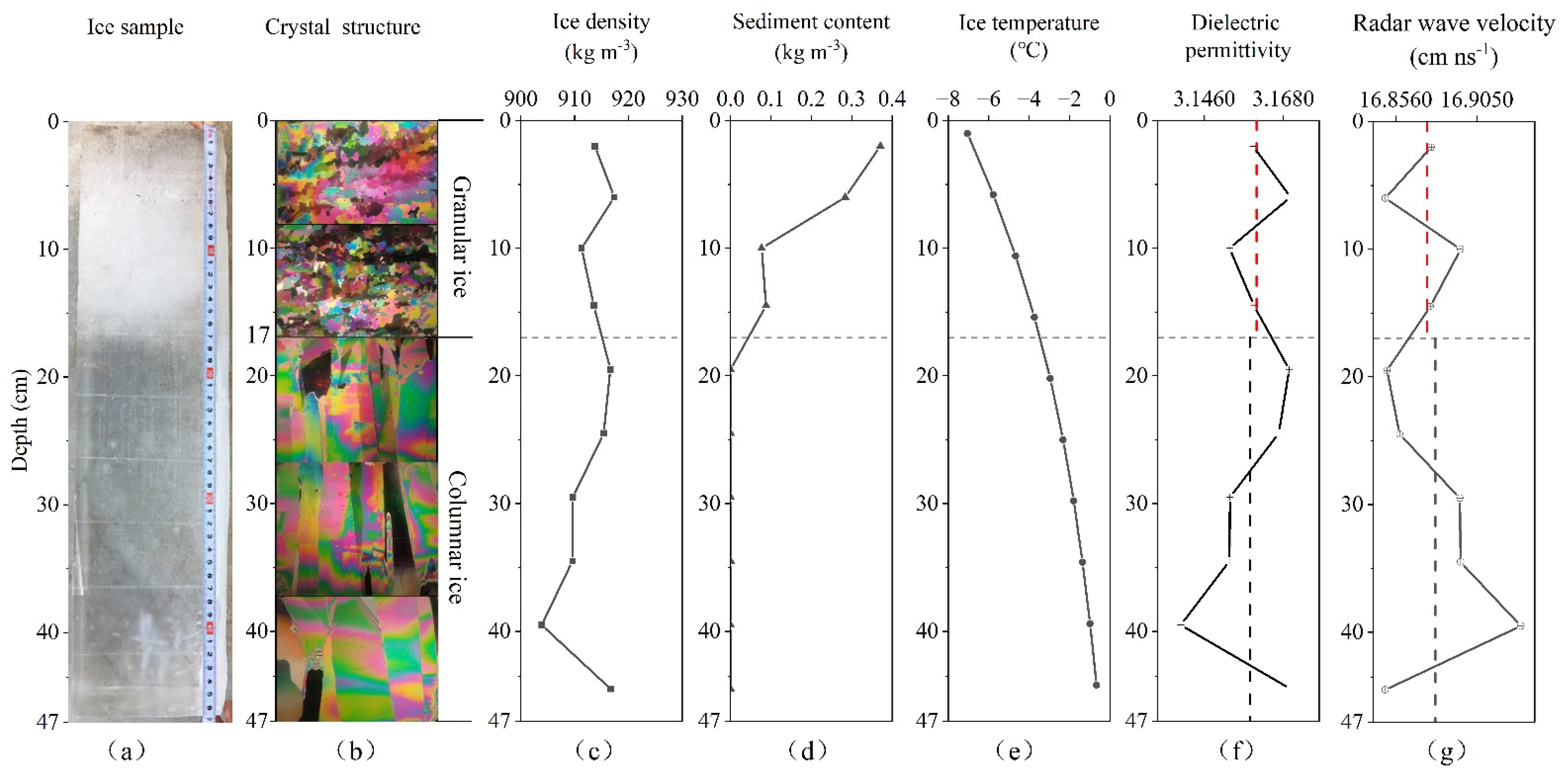
4.1. Ice Sample

In general, in a static body of water, granular ice exists within several centimeters of the primary ice surface layer, followed by columnar ice [32], for example Wuliangsu Lake ice in the Yellow River Basin [33]. However, granular ice occurred within 0–17 cm of the ice sample in the Yellow River, as shown in Figure 6b. Moreover, we observed that the ice sample in the granular ice was white and contained numerous bubbles (Figure 6a). This thick layer of granular ice did not belong to the primary ice of the static water body, according to the color and texture of the ice samples; rather, it must have been formed by the accumulation and freezing of frazil ice rather than the freezing of broken ice floes including sediment with a yellowish-brown color [22]. At 17–47 cm, the columnar ice shone brightly (Figure 6a). Additionally, the ice density of each ice layer ranged from 903.88 to 917.38 kg m⁻³, as shown in Figure 6c and

Table 1. Position of test center, mixture density, and sediment content of granular and columnar ice in the ice sample.

Crystal Structure	Position of Each Ice Layer Center (cm)	Measured Ice Block Density Including Pure Ice, Sediment, and Air (kg m−3)	Sediment Content per Unit Volume (kg m−3)
Granular ice	2	913.772	0.37
	6	917.381	0.28
	10	911.318	0.08
	14.5	913.563	0.09
Columnar ice	19.5	916.643	0
	24.5	915.418	0
	29.5	909.669	0
	34.5	909.606	0
	39.5	903.880	0
	44.5	916.728	0

. The sediment content of each ice layer ranged from 0 to 0.37 kg m⁻³, and a small quantity of sediments was contained only in granular ice but not in columnar ice, as shown in Figure 6d and Table 1. Figure 6e shows the ice temperature profile when cutting the ice sample. The unfrozen water in the ice sample was approximately 0 due to the low air temperature when testing the ice density and sediment. And the ice sample was clear and bright, with a small number of bubbles and sediment. The ice sample was regarded as a pure ice and bubble or pure ice, bubble, and sediment composite. Based on Equations (3) and (5), the dielectric permittivity (Figure 6f) of each ice layer, including granular or columnar ice, was calculated. Simultaneously, the radar wave velocity (Figure 6g) at each ice layer was calculated using Equation (2). Moreover, the volume ratio of each phase composition was evaluated on the premise of mass conservation, i.e., the volume ratio of bubbles [34]. The density, dielectric permittivity, and radar wave velocity of each phase composition, which were used to calculate the effective dielectric permittivity of each ice layer, are listed in

Table 2. Density, dielectric permittivity, and radar wave velocity of each phase substance.

Substance	Density (kg m−3)	Dielectric Permittivity	Radar Wave Velocity (m ns−1)	Source
Pure ice	917	3.17	0.1685	[4,9,11,35]
Air	0	1	0.3000	[4,9,11,35]
Pure water	1000	81	0.0333	[4,11,29,35]
Sediment	1800	5.50	0.1279	[35]

.

The results of the ice samples were normalized based on granular and columnar ice for their application as different types of ice in the Yellow River. The weighted average dielectric permittivity and radar wave velocity of granular and columnar ices were calculated according to the time spent by the radar wave passing through each layer of the ice sample. Figure 6f,g show the dielectric permittivity and radar wave velocity of each ice layer, respectively. The average dielectric permittivity of granular, sediment-containing granular, and columnar ice were calculated as 3.1605, 3.1607 (red vertical dotted line in Figure 6f), and 3.1586 (black vertical dotted line in Figure 6f), respectively, all of which were slightly smaller than that of pure ice (3.17) because bubbles were present in the Yellow River ice.

4.2. Natural Ice

On the premise of mass conservation, unfrozen water and ice crystals in the Yellow River ice replace each other dependent on the ice temperature. However, the dielectric permittivity may change substantially even with a minor change in the volume ratio of unfrozen water. Generally, the unfrozen water content in permafrost is determined using the measured dielectric permittivity [36,37,38], which develops into a dedicated radar detection technique for permafrost water contents [35]. Nevertheless, the unfrozen water content in ice has scarcely been evaluated based on the measured dielectric permittivity [39]. Although the unfrozen water content in ice with a small variation range presents a relatively simple relationship with the dielectric permittivity, it is nonlinearly correlated with the ice temperature, which is further nonlinearly correlated with the external environment factor. Despite the lack of literature supporting the measurement of the dielectric permittivity or radar wave velocity of natural ice directly using air temperature or a combination of air temperature and ice thickness, the statistical expressions of the parameters could be obtained through the large quantity of measured data collected in this study.

The feasibility of the parameterization scheme was first analyzed using ice thickness data measured 13 times. When the measured ice thickness was less than or equal to 17 cm, it was considered granular ice; moreover, if the measured ice thickness was greater than 17 cm, it was regarded as 17 cm granular and columnar ice. Then, the ice thickness was weighed according to the volume ratio of granular ice to columnar ice to assign the time spent by the radar wave passing through the two types of ice. On this basis, the mixing radar wave velocity was separated into granular and columnar ice containing unfrozen water. The unfrozen water content was calculated using Equations (3) and (5). Furthermore, the unfrozen water content, the ice temperature at the central position of the two types of ice (granular ice and columnar ice), and the air temperature were plotted in a scatter diagram (Figure 7). The central position was defined as the middle point of the thickness of the granular and columnar ice. For example, the central position for granular ice was 8.5 cm and that for columnar ice was the sum of the middle point of the columnar ice layer beneath the granular ice and the thickness of the granular ice. Figure 7 also shows the radar wave velocity differences between the two types of ice crystals. As shown in Figure 7a, the variation in the unfrozen water content in granular ice was larger than that in columnar ice, which ranged from 0 to 0.10 and from 0 to 0.01, respectively. This is because granular ice has more space between crystal grains and contains more unfrozen water. For the same unfrozen content in ice, the radar wave velocity of granular ice is higher than that of columnar ice, that is, the dielectric permittivity of granular ice is lower than that of columnar ice. There is a high correlation (r = 0.998) between the unfrozen water content and radar wave velocity. The unfrozen water content in ice is an important controlling factor of the radar wave velocity, especially in granular ice. In Figure 7b, the correlations between ice temperature and radar wave velocity in granular and columnar ice are 0.755 and 0.816, respectively. In Figure 7c, the scatters of granular and columnar ice approximately coincide. There is a low correlation (r = 0.457) between air temperature and radar wave velocity. Despite the correlation between air temperature and radar wave velocity in ice being relatively weak, the radar wave velocity changed within a small range (15.0–17.5 cm ns⁻¹) in spite of the wide range of variation of the air temperature from −24 °C to 8 °C. This shows that there is an indirect relationship between the air temperature and radar wave velocity in ice. Air temperature fluctuations have been shown to affect ice temperature changes, which control the unfrozen water content in ice. Hence, unfrozen water in ice was an important factor closely related to air temperature that determined the physically significant statistical relationship between air temperature and radar wave velocity.

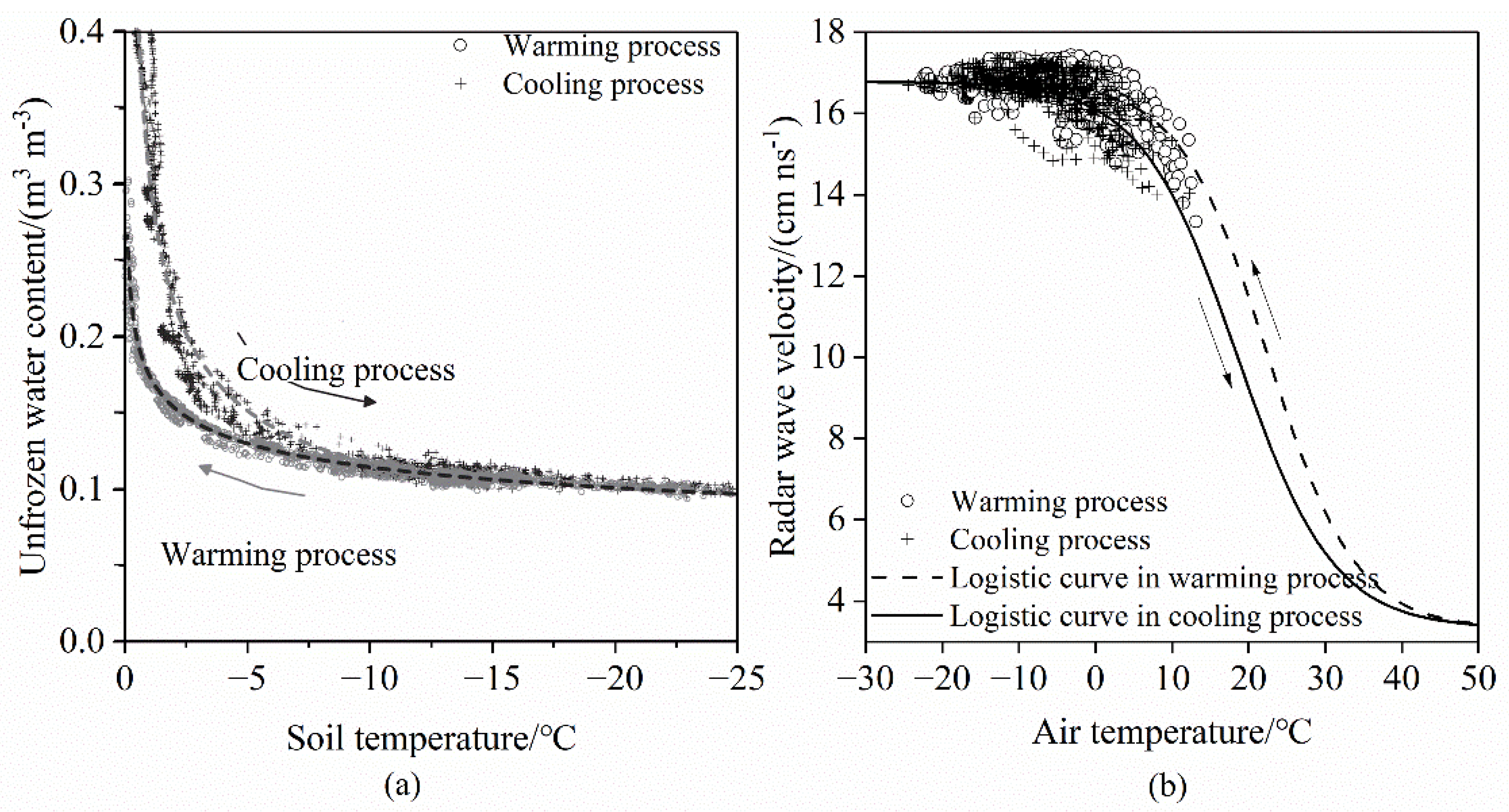
4.3. The Statistical Correction Expression for Radar Wave Velocity in Ice

Figure 7 confirms the feasibility and physical basis of the parameterization scheme of radar wave velocity correction with air temperature. Among the 13 manually measured ice thickness values, 12 were during the warming process of air temperature and 1 was the cooling process of air temperature. Manual measurements were primarily captured between 9:00 and 13:00, which only covered a limited scope of air temperature. In order to increase the statistics of the samples, we used the results of ice thickness simulation (the red dotted line in Figure 4b). Due to the support of measured ice thickness data between 30 December 2020 and 20 February 2021, 1251 simulated ice thicknesses during this period were selected for parametric scheme calculation. The timing of these data was consistent with the IGPR-50 radar detection time, and all were hourly. Of the 1251 ice thickness data, 578 were in the warming process of air temperature and 673 were in the cooling process of air temperature.

Given the existence of impurities in Yellow River water and the theory of phase transition in solutions, thermodynamic irreversibility occurs during the freezing and melting processes. For example, during the warming and cooling processes of saline frozen soil, the curve of the unfrozen water content in frozen soil varying with temperature is unclosed [40,41], as shown in Figure 8a. For this reason, radar wave velocity correction also considered the warming and cooling processes of the air temperature. That is, 590 ice thickness data, including 578 thermodynamic ice thicknesses and 12 manually measured ice thicknesses, were in the warming process of the air temperature, and 674 ice thickness data points, including 673 thermodynamic ice thicknesses and 1 manually measured value, were in the cooling process of the air temperature. They were then used to determine the relationship between air temperatures and radar wave velocities in granular and columnar ice, respectively, as the basis of radar wave velocity correction using air temperature. The radar wave velocity in the ice was lower than that in the frozen ice of the Yellow River and higher than that in the water of the Yellow River, displaying a nonlinear distribution according to the proportion of the two phases; thus, the logistic model was adopted here. Commonly used in mathematical statistics, this model is often applied to evaluate the carrying capacity of an environment and can also be used to analyze the change process of Arctic Sea ice coverage over time when the background is set as the icing time [42]. With three-phase (low-temperature ice, gas, and sediment) Yellow River ice and two-phase (high-temperature pure water and sediment) Yellow River water as the background, a four-parameter statistical expression was adopted as follows:

$$v_{\left(g or c\right)}=A/\left(1+C_1{e}^{D_1{\theta }_a}\right)+B,$$

(6)

where $v_{\left(g or c\right)}$ represents the radar wave velocity in granular or columnar ice, respectively; ${\theta }_a$ represents the air temperature; the sum of $A$ and $B$ indicates the radar wave velocity of three-phase Yellow River ice; $B$ indicates the radar wave velocity of two-phase Yellow River water, with A and B obtained by statistical optimization under theoretical guidance; and $C_1$ and $D_1$ represent the accommodation coefficient and logistic growth rate, respectively, both acquired via statistical optimization using the least squares method.

Equation (6) covers various types of Yellow River ice, such as flat, hummock, frazil, and broken ice within ice jams. Simultaneously, the radar wave velocity can conform to a physical basis. According to the 590 data in the warming process and 674 data in the cooling process, the logistic model for radar wave velocity correction was fitted and optimized (Figure 8b). The fitted warming process line (dotted line in Figure 8b) was higher than the fitted cooling process line (solid line in Figure 8b); in other words, under the same air temperature, the radar wave velocity during the warming process was larger than that during the cooling process. This is because the unfrozen water content in the cooling process is higher than that in the warming process under the same temperature, as shown in Figure 8a [40]. Liu et al. [4] indicated that unfrozen water in ice can slow the radar wave velocity; therefore, the logistic model shown in Figure 8b is consistent with the physical basis.

To expand the scope of application of radar wave velocity correction, we assigned radar wave velocity by weighing the thickness of the granular and columnar ices. The logistic models of air temperatures and radar wave velocities in the granular and columnar ice containing unfrozen water are displayed in Figure 9. The difference in the logistic curve in Figure 9a,b is the difference between coefficients C₁ and D₁ in Equation (6), as listed in

Table 3. Statistical coefficients and the correlation coefficient of different statistical methods.

Coefficients	Air Temperature				Air Temperature + Ice Thickness
	Warming Process		Cooling Process		Warming Process		Cooling Process
	GI *	CI *	GI *	CI *	GI *	CI *	GI *	CI *
A	13.6800	13.6800	13.6800	13.6800	13.4550	13.4550	13.4550	13.4550
B	3.3300	3.3300	3.3300	3.3300	3.6500	3.6500	3.6500	3.6500
C1	0.033	0.032	0.061	0.060	−0.892	−0.921	−6.813	−6.798
C2	0	0	0	0	7.229	7.436	48.376	48.271
C3	0	0	0	0	−16.98449	−17.48161	−110.36265	−110.12702
C4	0	0	0	0	12.343861	12.741714	81.956272	81.782522
D1	0.163	0.165	0.147	0.148	4.438	4.383	0.838	0.632
D2	0	0	0	0	−31.810	−31.345	−4.076	−2.504
D3	0	0	0	0	76.17527	74.89003	6.54336	2.56125
D4	0	0	0	0	−59.670671	−58.492396	−2.446005	0.906506
Correlation coefficient	0.7382	0.6884	0.7389	0.6884	0.8207	0.8210	0.8338	0.8338

*: granular ice (GI) and columnar ice (CI).

.

According to ice thermodynamics, the unfrozen water content in ice is the result of the combined effects of the air temperature and ice thickness. Although applying air temperature and radar-detected ice thickness to correct the radar wave velocity does not seem to conform to the theory, the mm/h-level change in thermodynamic ice thickness allows the radar wave velocity to be corrected by the previous ice thickness for any frozen ice, which is technically and mathematically feasible. Topp’s cubic model, Roth’s cubic model, and Herkelrath’s one-half power and polynomial models were adopted for the unfrozen water content and dielectric coefficient [34,35,37], while a polynomial model was adopted for temperature and dielectric permittivity [36,43]. Therefore, coefficients $C_1$ and $D_1$ in Equation (6) were corrected using the third power of the ice thickness, and thus Equations (7) and (6) are consistent with contemporary mathematics. In this way, when only the effects of air temperature were considered, coefficients $C_1$ and $D_1$ were not equal to zero, whereas coefficients $C_2$, $C_3$, $C_4$, $D_2$, $D_3$, and $D_4$ were all equal to zero, indicating a problem of constant coefficients. When the previous ice thickness was also added to the correction based on air temperature, coefficients $C_1$, $C_2$, $C_3$, $C_4$, $D_1$, $D_2$, $D_3$, and $D_4$ were not equal to zero, indicating a problem with the functions. The number of decimal places of the coefficients was determined based on the prerequisite that the radar wave velocity was guaranteed to retain four decimal places.

$$v_r=A/(1+\left(C_1+C_{2}h+C_3{h}^2+C_4{h}^3\right)e^{\left(D_1+D_{2}h+D_3{h}^2+D_4{h}^3\right){\theta }_a})+\mathrm{B},$$

(7)

where $h$ represents the previous ice thickness, and the other symbols are the same as in Equation (6).

Based on Equation (7), the multiple correlation statistics of air temperature, ice thickness, and radar wave velocity were fitted and optimized using the least squares method, as shown in Figure 10. The difference between the fitted surface in granular (Figure 10a,b) and columnar ice (Figure 10c,d) is the difference in coefficients C₁, C₂, C₃, C₄, D₁, D₂, D₃, and D₄ in Equation (7), as listed in Table 3.

After adding the ice thickness correction, whether it was granular or columnar ice during the warming and cooling periods, the fitting correlation coefficients all increased accordingly (Table 3). The smallest correlation coefficients of the two correction methods (Equations (6) and (7)) increased from 0.6884 to 0.8207. For better observation of the correction effects, an error analysis of no correction, correction by air temperature, and correction by air temperature and the previous ice thickness was conducted based on the 578 and 673 radar-detected ice thicknesses and thermodynamically simulated ice thicknesses in the warming and cooling processes. Figure 11 illustrates the effect before and after ice thickness correction using Equations (6) and (7).

Table 4. Correlation coefficient and errors of the simulated and measured ice thickness after correction and the radar-detected ice thickness before and after correction.

Indicator		No Correction	Correction by Air Temperature	Correction by Air Temperature and Ice Thickness
Cooling process	Correlation coefficient r	0.97181	0.98577	0.99164
	MSEs	0.00026	0.00016	0.00015
	RMSEs	0.01608	0.01249	0.01205
	MAEs	0.01050	0.00958	0.01003
Warming process	Correlation coefficient r	0.97584	0.99010	0.99192
	MSEs	0.00025	0.00013	0.00015
	RMSEs	0.01596	0.01132	0.01209
	MAEs	0.01069	0.00880	0.01004

shows the statistical correlation coefficients (r), mean square errors (MSEs), root mean square errors (RMSEs), and mean absolute errors (MAEs). Notably, compared with no correction, better effects were observed after the corrections. Correction by air temperature demonstrated significant effects because air temperature was the dominant factor controlling the unfrozen water content in ice, which was revealed by the observable improvement in correlation coefficient and errors in Table 4. Ice thickness was the secondary factor controlling the unfrozen water content in ice, so correction by air temperature and ice thickness accorded with theoretical analysis; however, its response to the correlation coefficient and errors was at the same level as the correction by air temperature.

5. Discussion

Based on this study and previous research results and experiences, the following suggestions or discussions are proposed:

• To correct the radar wave velocity by air temperature and ice thickness in future practice, the following steps should be followed. (a) Previous ice thicknesses and air temperatures should be recorded. (b) Air temperature during calibration should be measured. (c) The difference between these previous and measured air temperatures should be calculated. (d) When a positive result is obtained from step (c), the correction coefficient of the warming process in Table 3 should be selected, while when a negative result is obtained, the correction coefficient of the cooling process should be selected, as shown in Table 3. Finally, (e) according to the correction coefficient of step (d), the current radar wave velocity should automatically be calculated using Equation (7), and the ice thickness should also be automatically calculated. If the test is taken for the first time, the researcher is advised to use the ideal radar wave velocity in ice for the first time, repeat the test five times following steps (a)–(b), and take the ice thicknesses measured for the last time;
• The unfrozen water content in ice is the core factor controlling radar wave velocity. Theoretically, air temperature is the main influence factor of radar wave velocity through ice temperature (Equation (6)), and ice thickness is the secondary influence factor of ice temperature. The combined effect of air temperature and ice thickness on radar wave velocity (Equation (7)) does not perform significantly better than Equation (6). If the accuracy requirement is not very high, the simple Equation (6) is enough. Using the unfrozen water content to evaluate the radar wave velocity is basic research, except for the GPR results of inversed unfrozen water fractions in ice [20,21], which can be inversed under controlled temperature in laboratory using X-ray computed tomography (CT) [44,45] and magnetic resonance imaging (MRI) [46,47]. Both technologies can obtain the volume fractions of different phases but cannot give the fixed index because there are different chemical materials in air and water. These chemical materials also make the index vary in a certain range [48]. We have used CT scan technology to measure ice samples from Bohai, the Arctic, and Wuliangsu Lake near the Yellow River since 1994 [49,50,51]. However, the objectives of obtaining the phase volume from fraction were not achieved. We will continue this study after we have new types of CT scanner later;
• In addition, the grain boundary also affects unfrozen water content; the more grain boundaries, the more unfrozen water content for a given ice temperature. The effect of grain size on the unfrozen water content is the new direction of future efforts. Lastly, solar radiation, cloud cover and wind speed also affect the vertical ice temperature profile. It is necessary to use ice thermodynamic models to calculate the ice temperature. In fact, these thermodynamic models have been continuously modified through the effort to cover the middle and high latitudes, such as the contributions from Cheng (2021) [52], and the parameterizations for the daily ice surface albedos for clear days and cloudy days also were explored [53]. At present, for the cases of polar and high-latitude ice with local cloud, solar radiation, and wind features, it is not necessary to correct radar wave velocity in real time, but radar wave velocity can instead be corrected in periods, such as the early freezing period, growth period, and thaw period. In the future, the new modification method will be developed based on ice thermodynamic models;
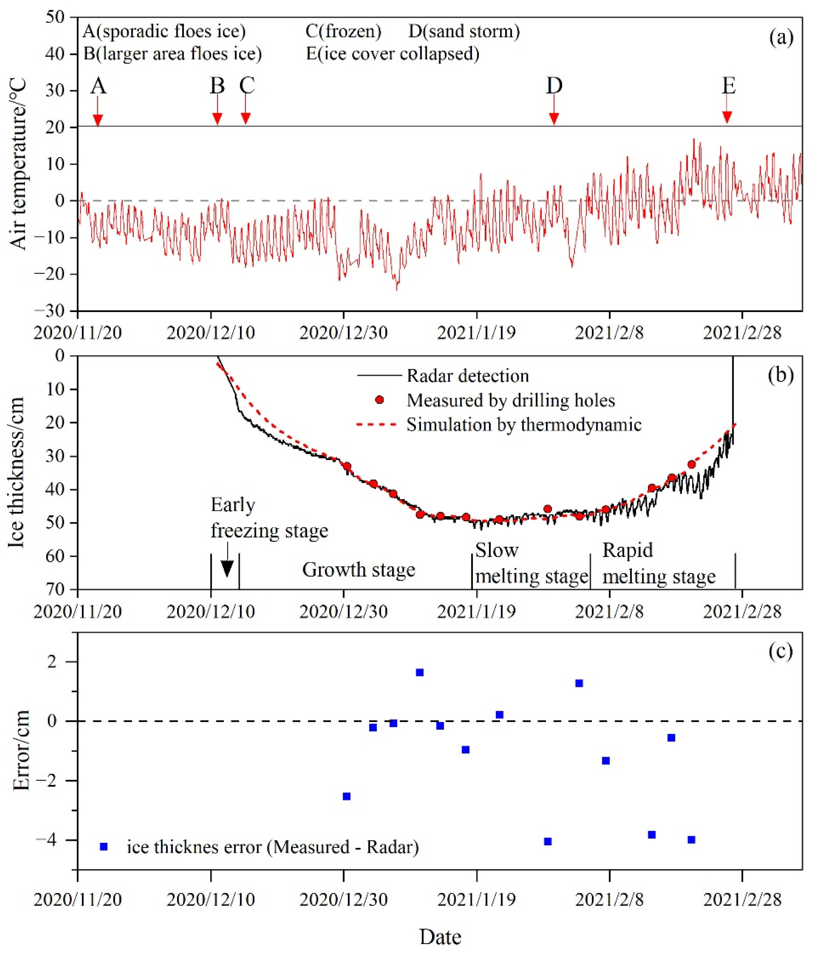
• Thirteen manually measured ice thicknesses were inadequate for statistical analysis using the measured ice thicknesses directly. A thermodynamic model was employed to simulate ice thickness; however, the thermodynamic model failed to produce satisfactory results for the dynamic ice thickness variations. In particular, the heat flux of the ice–water interface might vary in different areas of the Yellow River. Thus, it is necessary to consider that both thermodynamics and dynamics contributed to the practical ice thickness of the Yellow River, especially for the unfrozen frazil ice and accumulated broken ice in ice jams in the Yellow River, which possess a high content of unfrozen water. This shows that current statistical parameters do not include measured data of these areas with high water content, and corrections to such areas may thus fall short of high precision. To address this issue, ongoing research and opportunities are required. In future research, the following should be considered: (a) When experimenting with a fixed H–GPR–S, attention should be paid to granular, columnar, and frazil ice in the ice layers and the occurrence of flowing frazil ice and stacked broken ice beneath the ice cover. Additionally, a high-precision sensor for measuring ice thickness and temperature should be installed beneath and inside of the ice, respectively. Sensors for testing frazil and stacked broken ice should be developed under the ice layers. (b) When experimenting with a mobile towing radar, notes should be made on the difference in ice crystal structure in vertical sections of ice layers at every measuring point, particularly the difference in the distribution location and sediment content, and the water content characteristics of frazil ice and stacked broken ice. If sediment content in ice changes with time and position, the dielectric permittivity of ice needs to be reevaluated. However, for floating ice, the sediment content in ice is difficult to measure quickly. When floating ice freezes into ice cover, the sediment content of the floating ice in different places can be measured [22]. We plan to first try to normalize the sediment content for different ice types at different locations in Yellow River, and then the influence of sediment content in ice on the dielectric permittivity will be considered in future efforts. (c) In the future, both radar-detected data and physically measured ice layer data [4,33] will be available and sufficiently accumulated. Such data and the theoretical basis presented in this paper should be applied to build statistical correction coefficients for multiple types of radar wave velocities in ice, which encompasses the thermodynamic and dynamic effects in winter for the Yellow River;
• When thermal growth of ice thickness is detected via a mobile towing radar, a sensor for air temperature should be used. Because manual measurements are often performed during the day when the air temperature is warm, the correction coefficient of air temperature and ice thickness in the warming process should be adopted. For hummock and frazil ice frozen in the Yellow River, the statistics for granular ice should be used. For lake ice, columnar ice statistics should be used, while for flat ice after the ice floes stop moving, the weighted result of granular ice on the 0.15 m of the surface layer and the other columnar ice should be used; in the future, fixed H–GPR–S experiments in other rivers should not be conducted by detecting flat ice and avoiding hummock ice. Instead, both should be selected in the same terrain and meteorological environment so that scientific data can be accumulated to determine the influences of the structure and component differences of flat ice and hummock ice on the high-precision radar detection of ice thickness.

6. Conclusions

In addition to bubbles, naturally frozen ice in the Yellow River also contains sediment impurities and unfrozen water and is displayed as four-phase (pure ice–bubble–sediment–unfrozen water), three-phase (pure ice–bubble–sediment), or two-phase (pure ice–bubble) composite materials that vary with ice temperature. When unfrozen water in ice was absent, the flat ice in the Shisifenzi bend exhibited the following dielectric permittivity: 3.1605 for granular ice, 3.1607 for granular ice containing sediment, and 3.1586 for columnar ice; all of these are slightly smaller than the dielectric permittivity (3.17) of pure ice reported in another paper. In addition, to ensure the precision of the radar detection thickness (1 mm), the number of decimal places of the ice dielectric permittivity and radar wave velocities needed to be raised from two or three to four.

The radar wave velocity was overestimated when unfrozen water was present in the ice. For the fixed H–GPR–S in the Shisifenzi bend in the Yellow River, the frequencies and phases of the daily variation of the measured air temperature and the radar-detected flat ice thickness evidence that air temperature was the most important factor among all external environment factors influencing unfrozen water content in ice. Thus, setting the radar wave velocity to a constant value unaffected by the change in air temperature will reduce the precision of ice thickness detection for radar at high air temperatures during freezing and thawing periods.

Through theoretical analysis, we found a physical relationship between air temperature and unfrozen water content in ice, indicating the necessity of adopting correction by air temperature. Furthermore, the combination of air temperature and ice thickness has a clear relationship with unfrozen water content in the ice. Although the correction by air temperature and ice thickness was at the same precision level as the correction by air temperature, the correction by air temperature and ice thickness should be adopted as the parameterization of correcting radar wave velocity in ice.

For hummock ice and frazil ice frozen in the Yellow River, parameterization of granular ice should be used. For lake ice, a parametrization of columnar ice should be used. For flat ice after the ice flow stops moving, the important result of granular ice on the 15 cm of the surface layer and the other columnar ice should be used.

References

- Zhou, L.; Yu, D.; Wang, Z.Y.; Wang, X. Soil water content estimation using high-frequency ground penetrating radar. Water 2019, 11, 1036. [Google Scholar] [CrossRef] [Green Version]
- Abdelmawla, A.; Kim, S.S. Application of ground penetrating radar to estimate subgrade soil density. Infrastructures 2020, 5, 12. [Google Scholar] [CrossRef] [Green Version]
- Ruffell, A.; Parker, R. Water penetrating radar. J. Hydrol. 2021, 597, 126300. [Google Scholar] [CrossRef]
- Liu, J.; Wang, S.; He, Y.; Li, Y.; Wang, Y.; Wei, Y.; Che, Y. Estimation of ice thickness and the features of subglacial media detected by ground penetrating radar at the Baishui river glacier No. 1 in Mt. Yulong, China. Remote Sens. 2020, 12, 4105. [Google Scholar] [CrossRef]
- Shah, M.Y.; Ayemi, K.K.; Shrivastava, P.K. GPR survey and physical measurements of sea ice in Quilty Bay, Larsemann hills, East Antarctica and its correlation with local atmospheric parameters. J. Geol. Soc. India 2017, 90, 371–377. [Google Scholar] [CrossRef]
- O’Sadnick, M.; Ingham, M.; Eicken, H.; Pettit, E. In situ field measurements of the temporal evolution of low-frequency sea-ice dielectric properties in relation to temperature, salinity, and microstructure. Cryosphere 2016, 10, 2923–2940. [Google Scholar] [CrossRef] [Green Version]
- Mitterer, C.; Heilig, A.; Schweizer, J.; Eisen, O. Upward-looking ground-penetrating radar for measuring wet-snow properties. Cold Reg. Sci. Technol. 2011, 69, 129–138. [Google Scholar] [CrossRef]
- Sudakova, M.; Sadurtdinov, M.; Skvortsov, A.; Tsarev, A.; Malkova, G.; Molokitina, N.; Romanovsky, V. Using ground penetrating radar for permafrost monitoring from 2015–2017 at CALM Sites in the Pechora River Delta. Remote Sens. 2021, 13, 3271. [Google Scholar] [CrossRef]
- Arcone, S.A.; Delaney, A.J. Airborne river-ice thickness profiling with helicopter-borne UHF short-pulse radar. J. Glaciol. 1987, 33, 330–340. [Google Scholar] [CrossRef] [Green Version]
- Arcone, S.A. Dielectric permittivity and layer-thickness interpretation of helicopter-borne short-pulse radar waveforms reflected from wet and dry river-ice sheets. IEEE Geosci. Remote 1991, 29, 768–777. [Google Scholar] [CrossRef]
- Li, Z.; Jia, Q.; Zhang, B.; Leppäranta, M.; Lu, P.; Huang, W. Influences of gas bubble and ice density on ice thickness measurement by GPR. Appl. Geophys. 2010, 7, 105–113. [Google Scholar] [CrossRef]
- Liu, H.; Sato, M. New GPR system for accurate velocity and thickness estimation of snow and ice on a frozen lake. In Proceedings of the 10th SEGJ International Symposium, Kyoto, Japan, 20–22 November 2011. [Google Scholar] [CrossRef]
- Liu, H.; Xie, X.; Sato, M. New ground penetrating radar system for quantitative characterization of snow and sea ice. In Proceedings of the IET International Radar Conference 2013, Xi’an, China, 14–16 April 2013. [Google Scholar] [CrossRef]
- Liu, H.; Takahashi, K.; Sato, M. Measurement of Dielectric Permittivity and Thickness of Snow and Ice on a Brackish Lagoon Using GPR. IEEE J-STARS 2014, 7, 820–827. [Google Scholar] [CrossRef]
- Gusmeroli, A.; Grosse, G. Ground penetrating radar detection of subsnow slush on ice-covered lakes in interior Alaska. Cryosphere 2012, 6, 1435–1443. [Google Scholar] [CrossRef] [Green Version]
- Zhang, B.; Zhang, F.; Liu, Z.; Han, H.; Li, Z. Field experimental study of the characteristics of GPR images of Yellow River ice. South-To-North Water Transfers Water Sci. Technol. 2017, 15, 121–125. (In Chinese) [Google Scholar] [CrossRef]
- Kämäri, M.; Alho, P.; Colpasert, A.; Lotsari, E. Spatial vaiation of river ice thickness in meandering river. Cold Reg. Sci. Technol. 2017, 137, 17–29. [Google Scholar] [CrossRef]
- Fu, H.; Liu, Z.; Guo, X.; Cui, H. Double-frequency ground penetrating radar for measurement of ice thickness and water depth in rivers and canals: Development, verification and application. Cold Reg. Sci. Technol. 2018, 154, 85–94. [Google Scholar] [CrossRef]
- Bai, X.; Wang, L.; Luo, X.; Mi, H.; Chen, H.; Liu, L.; Ji, M.; Gao, Y. A layer tracking method for ice thickness detection based on GPR mounted on the UAV. In Proceedings of the 4th International Conference on Imaging, Signal Processing and Communications (ICISPC), Kumamoto, Japan, 23–25 October 2020. [Google Scholar] [CrossRef]
- Murray, T.; Stuart, G.W.; Fry, M.; Gamble, N.H.; Crabtree, M.D. Englacial water distribution in a temperate glacier from surface and borehole radar velocity analysis. J. Glaciol. 2000, 46, 389–398. [Google Scholar] [CrossRef] [Green Version]
- Murray, T.; Booth, A.D.; Rippin, D. Water-content of glacier-ice: Limitations on estimates from velocity analysis of surface ground penetrating radar surveys. J. Environ. Eng. Geoph. 2007, 12, 87–99. [Google Scholar] [CrossRef]
- Zhang, Y.; Li, Z.; Xiu, Y.; Li, C.; Zhang, B.; Deng, Y. Microstructural characteristics of frazil particles and the physical properties of frazil ice in the Yellow River, China. Crystals 2021, 11, 617. [Google Scholar] [CrossRef]
- Launiainen, J.; Cheng, B. Modelling of ice thermodynamics in natural water bodies. Cold Reg. Sci. Technol. 1998, 27, 153–178. [Google Scholar] [CrossRef]
- Li, C.; Li, Z.; Yang, Y.; Wang, Q.; Zhang, B.; Deng, Y. Theory and application of ice thermodynamics and mechanics for sinking naturally gabions mattress on ice. J. Hydraul. Eng. 2022, 53, 445–455. (In Chinese) [Google Scholar] [CrossRef]
- Ji, H.; Shi, H.; Mou, X.; Tuo, Y. Study on the pool ice growth-decay and numerical modeling. J. Hydraul. Eng. 2016, 47, 1352–1362. (In Chinese) [Google Scholar] [CrossRef]
- Lu, P.; Cao, X.; Li, G.; Huang, W.; Leppäranta, M.; Arvola, L.; Huotari, J.; Li, Z. Mass and heat balance of a lake ice cover in the Central Asian Arid Climate Zone. Water 2020, 12, 2888. [Google Scholar] [CrossRef]
- Evans, S. Dielectric properties of ice and snow: A review. J. Glaciol. 1965, 5, 773–792. [Google Scholar] [CrossRef] [Green Version]
- Koh, G. Complex dielectric permittivity of ice at 1.8 GHz. Cold Reg. Sci. Technol. 1997, 25, 119–121. [Google Scholar] [CrossRef]
- Lunt, I.A.; Hubbard, S.S.; Rubin, Y. Soil moisture content estimation using ground-penetrating radar reflection data. J. Hydrol. 2005, 307, 254–269. [Google Scholar] [CrossRef]
- Xu, Q.; Yan, X.; Grantz, D.; Wang, Z.; Cheng, X.; Yu, S.; Fan, L.; Ma, Y.; Cheng, Q. An ice correction model for dielectric sensor to improve accuracy of soil water potential measurement in frozen soils. Soil Till. Res. 2021, 211, 105003. [Google Scholar] [CrossRef]
- Shokr, M.E. Field observations and model calculations of dielectric properties of Arctic sea ice in the microwave C-band. IEEE Geosci. Remote 1998, 36, 463–478. [Google Scholar] [CrossRef]
- Michel, B. Ice Mechanics; Laval University Press: Laval, QC, Canada, 1978; pp. 124–136. [Google Scholar]
- Zhang, Y.; Gao, G.; Deng, Y.; Li, Z.; Li, G.; Guo, W. Investigation on ice crystal, density and sediment content in ice at different positions in Bayannaoer section of the Yellow River. Yellow River 2018, 40, 44–48. (In Chinese) [Google Scholar] [CrossRef]
- Gherboudj, I.; Bernier, M.; Hicks, F.; Leconte, R. Physical characterization of air inclusions in river ice. Cold Reg. Sci. Technol. 2007, 49, 179–194. [Google Scholar] [CrossRef]
- Guo, Y.; Xu, S.; Shan, W. Development of a frozen soil dielectric permittivity model and determination of dielectric permittivity variation during the soil freezing process. Cold Reg. Sci. Technol. 2018, 151, 28–33. [Google Scholar] [CrossRef]
- Roth, K.; Schulin, R.; Flühler, H.; Attinger, W. Calibration of time domain reflectometry for water content measurement using a composite dielectric approach. Water Resour. Res. 1990, 26, 2267–2273. [Google Scholar] [CrossRef]
- Alharthi, A.; Lange, J. Soil water saturation: Dielectric determination. Water Resour. Res. 2010, 23, 591–595. [Google Scholar] [CrossRef]
- Herkelrath, W.N.; Hamburg, S.P.; Murphy, F. Automatic, real-time monitoring of soil moisture in a remote field area with time domain reflectometry. Water Resour. Res. 1991, 27, 857–864. [Google Scholar] [CrossRef]
- Fabbri, A.; Fen-Chong, T.; Coussy, O. Dielectric capacity, liquid water content, and pore structure of thawing-freezing materials. Cold Reg. Sci. Technol. 2006, 44, 52–66. [Google Scholar] [CrossRef]
- Overduin, P.P.; Kane, D.L.; van Loon, W.K.P. Measuring thermal conductivity in freezing and thawing soil using the soil temperature response to heating. Cold Reg. Sci. Technol. 2006, 45, 8–22. [Google Scholar] [CrossRef] [Green Version]
- Wang, C.; Lai, Y.; Yu, F.; Li, S. Estimating the freezing-thawing hysteresis of chloride saline soils based on the phase transition theory. Appl. Therm. Eng. 2018, 135, 22–33. [Google Scholar] [CrossRef]
- Duan, C.; Dong, S.; Wang, Z. Study on arctic sea Ice growth based on Logistic curve model. T. Oceanol. Limn. 2021, 4, 1–6. (In Chinese) [Google Scholar] [CrossRef]
- Zhao, G.; Qiao, C.; Yan, Y.; Feng, F.; Wang, L.; Zhang, S.; Chen, Y. Study on model of relations between water content and dielectric constant: Experimental study. Hydrogeol. Eng. Geol. 2016, 43, 7–10. (In Chinese) [Google Scholar] [CrossRef]
- Kawamura, T. Observations of the internal structure of sea ice by X ray computed tomography. J. Geophys. Res. Atmos. 1988, 93, 2243–2350. [Google Scholar] [CrossRef]
- Lieb-Lappen, R.M.; Golden, E.J.; Obbard, R.W. Metrics for interpreting the microstructure of sea ice using X-ray micro-computed tomography. Cold Reg. Sci. Technol. 2017, 138, 24–35. [Google Scholar] [CrossRef]
- Eicken, H.; Bock, C.; Wittig, R.; Miller, H.; Poertner, H.O. Magnetic resonance imaging of sea ice pore fluids: Methods and thermal evolution of pore microstructure. Cold Reg. Sci. Technol. 2000, 31, 207–225. [Google Scholar] [CrossRef] [Green Version]
- Brown, J.R.; Brox, T.I.; Vogt, S.J.; Seymour, J.D.; Skidmore, M.L.; Codd, S.L. Magnetic resonance diffusion and relaxation characterization of water in the unfrozen vein network in polycrystalline ice and its response to microbial metabolic products. J. Magn. Reson. 2012, 225, 17–24. [Google Scholar] [CrossRef]
- Crabeck, O.; Galley, R.; Delille, B.; Else, B.; Geilfus, N.; Lemes, M.; Roches, M.D.; Francus, P.; Tison, J.; Rysgaard, S. Imaging air volume fraction in sea ice using non-destructive X-ray tomography. Cryosphere 2016, 10, 1125–1145. [Google Scholar] [CrossRef] [Green Version]
- Li, Z.; Pu, Y.; Gao, S.; Liao, Q. Images of computerized tomography in nature sea ice in Liaodong Gulf. In Proceedings of the Abstracts of 9th International Symposium on Okhotsk Sea and Sea Ice, Mombetsu, Japan, 6–8 February 1994. [Google Scholar]
- Li, Z.; Pu, Y. Some applications of computerized tomography scanner to sea ice. In Proceedings of the Twelfth International Offshore and Polar Engineering Conference, Kitakyushu, Japan, 26–31 May 2002. [Google Scholar]
- Wang, S.; Li, Z.; Zhang, Y.; Xiu, Y.; Deng, Y.; Li, G. A preliminary study on observations of the fabric of lake ice by CT scanning technique. Hydro. Sci. Cold Zone Eng. 2020, 3, 63–69. (In Chinese) [Google Scholar] [CrossRef]
- Cheng, B.; Vihma, T.; Palo, T.; Nicolaus, M.; Gerland, S.; Rontu, L.; Haapala, J.; Perovich, D. Observation and modelling of snow and sea ice mass balance and its sensitivity to atmospheric forcing during spring and summer 2007 in the Central Arctic. Adv. Polar Sci. 2021, 32, 312–326. [Google Scholar] [CrossRef]
- Li, Z.; Wang, Q.; Tang, M.; Lu, P.; Li, G.; Leppäranta, M.; Huotari, J.; Arvola, L.; Shi, L. Diurnal Cycle Model of Lake Ice Surface Albedo: A Case Study of Wuliangsuhai Lake. Remote Sens. 2021, 13, 3334. [Google Scholar] [CrossRef]