Tree Segmentation and Parameter Measurement from Point Clouds Using Deep and Handcrafted Features

Abstract

Accurate measurement of the geometric parameters of trees is a vital part of forest inventory in forestry management. Aerial and terrestrial Light Detection and Ranging (LiDAR) sensors are currently used in forest inventory as an effective and efficient means of forest data collection. Many recent approaches to processing and interpreting this data make use of supervised machine learning algorithms such as Deep Neural Networks (DNNs) due to their advantages in accuracy, robustness and the ability to adapt to new data and environments. In this paper, we develop new approaches to deep-learning-based forest point cloud analysis that address key issues in real applications in forests. Firstly, we develop a point cloud segmentation framework that identifies tree stem points in individual trees and is designed to improve performance when labelled training data are limited. To improve point cloud representation learning, we propose a handcrafted point cloud feature for semantic segmentation which plays a complementary role with DNNs in semantics extraction. Our handcrafted feature can be integrated with DNNs to improve segmentation performance. Additionally, we combine this feature with a semi-supervised and cross-dataset training process to effectively leverage unlabelled point cloud data during training. Secondly, we develop a supervised machine learning framework based on Recurrent Neural Networks (RNNs) that directly estimates the geometric parameters of individual tree stems (via a stacked cylinder model) from point clouds in a data-driven process, without the need for a separate procedure for model-fitting on points. The use of a one-stage deep learning algorithm for this task makes the process easily adaptable to new environments and datasets. To evaluate our methods for both the segmentation and parameter estimation tasks, we use four real-world datasets of different tree species collected using aerial and terrestrial LiDAR. For the segmentation task, we extensively evaluate our method on the three different settings of supervised, semi-supervised, and cross-dataset learning, and the experimental results indicate that both our handcrafted point cloud feature and our semi-supervised and cross-dataset learning framework can significantly improve tree segmentation performance under all three settings. For the tree parameter estimation task, our DNN-based method performs comparably to well-established traditional methods and opens up new avenues for DNN-based tree parameter estimation.

1. Introduction

Forest terrains constitute more than 30% of the Earth’s landmass and serve multiple functionalities to local and global ecosystems as well as society including maintaining biodiversity, mitigating climate changes, and being of economic value. Forest inventory technologies play an essential role in investigating and managing natural and commercial forests. Traditionally, forest inventory relies on manual field work which is laborious and time-consuming. In recent years, with the development of laser scanning technology, Light Detection and Ranging (LiDAR) devices have been increasingly adopted in automatic forest inventory as a more convenient means of tree data acquisition [1,2,3,4,5,6], and current studies are using LiDAR devices mounted on several types of platforms (e.g., mobile terrestrial platforms, manned aircraft, and unoccupied aerial systems) for forests of different scales (e.g., plot, stand, and regional).

When determining the characteristics of individual trees based on LiDAR point clouds, the first and most important task is to locate the main stem of each tree. For data-driven methods, the main method for this task is point cloud semantic segmentation which is used to separate stem points from foliage points. Most recently, following the prevalence of deep neural networks (DNNs) in machine learning and computer vision research, several tree point cloud segmentation methods based on existing general-purpose DNN segmentation models have been proposed and promising results have been reported [7,8,9,10,11]. The other important task in LiDAR-based automatic forest inventory is tree parameter estimation, in which the segmented stem and foliage points are used for estimating several relevant tree parameters including height, basal area, diameter at breast height (DBH), and taper. These parameters are typically estimated using model-fitting techniques, including circular cross-sections or the use of cylinder shape models [10,12,13,14]. Methods for shape fitting must typically be designed for, or tuned towards, a specific type and resolution of point cloud data.

Despite the progress made by existing research, both tree point cloud segmentation and tree parameter estimation techniques still face a few challenges. For tree point cloud segmentation, one issue is that existing works have been mainly employing the general-purpose methods that were originally designed for the scenarios of autonomous driving, indoor scene, and general artificial object partitioning [15,16,17,18,19,20,21,22], while these methods may not be optimal for a forest scenario. More specifically, point cloud objects in autonomous driving and robotic navigation scenarios have more regular surfaces than trees, while trees usually have a higher degree of variation in geometric shape which makes tree point cloud segmentation challenging. The other issue in tree point cloud segmentation is that forest point clouds are highly structurally complex and heterogeneous in general, which makes manual labelling very difficult. Therefore, large-scale and publicly-accessible labelled datasets are not currently available, making labelled training data scarce. Furthermore, because of the shortage of labelled training data, DNN-based semantic segmentation models may learn feature representations that are ineffective. Additionally, it is often the case in a real forestry application that models may be trained using data from one site/forest type and used to process tree point cloud data in a new site, without wanting to expend the effort of hand-labelling additional training examples from the new site. For tree parameter estimation, it would be advantageous to design a data-driven approach that can be easily used for different types of tree point clouds (e.g., those of different species or captured with different types of LiDAR) while can also exploit the variety of data for more accurate estimation.

To address the issues above, we propose methods to improve forest point cloud semantic segmentation and introduce a DNN-based data-driven framework for tree parameter estimation. We summarise the contributions of our work as follows:

• Inspired by the success of existing works which jointly utilise DNN and handcrafted features for better image and point cloud representations [23,24,25,26], we propose a handcrafted feature method which can extract more explicit information than DNNs, particularly in scenarios in which labelled training data is scarce. Our handcrafted feature extractor performs on par with DNN models on the tree point cloud segmentation tasks. Based on our handcrafted feature, we further proposed the first point cloud semantic segmentation model for forest point clouds which outperforms the DNN baselines by combining the advantages of both DNN and a handcrafted feature.
• To deal with the practical situations where we only have access to a limited amount of labelled tree point clouds, we propose a semi-supervised learning framework that can effectively exploit unlabelled point cloud data of trees for training the segmentation model. Moreover, our semi-supervised learning framework can be easily extended to a domain adaptation setting to deal with the cross-dataset semantic segmentation problem. To the best of our knowledge, this is the first work to tackle the point cloud semantic segmentation problem in forests by utilising unlabelled data for training learning models, while our framework is versatile and can be used under both semi-supervised learning and domain adaptation settings.
• To achieve better robustness and adaptability in the tree parameter estimation task, we propose the first DNN-based tree parameter estimation framework which estimates the tree model parameters directly from input point clouds. The use of our data-driven framework for the tree parameter estimation task allows for a method that can adapt to the specifics of the training data examples provided.

Extensive experimental results on four different real-world datasets demonstrate the effectiveness of all our proposed methods, i.e., the handcrafted feature method, the semantic segmentation model which integrates handcrafted feature with DNN, the semi-supervised learning and domain adaptation framework, and the DNN-based tree parameter estimation method.

The rest of the paper is organised as follows. In Section 2, we discuss related work. In Section 3, we introduce our proposed method in detail. Experimental results are presented in Section 4 and conclusions of our work in Section 5.

2. Related Work

2.1. Tree Parameter Estimation from LiDAR Point Clouds

Three-dimensional forest point cloud data can be used to automatically determine key inventory metrics at a tree-by-tree level via a variety of different methods, depending on the resolution and coverage of the data. Over the broad scales and low-resolution typical of airborne LiDAR where structural characteristics are not directly observable, tree stem properties may be inferred indirectly via linear model fitting [27], imputation methods [28] or copulas [29] from the pattern of points present, for example, in the tree canopy. For high-resolution point clouds in which stem points are directly observable, parametric model-fitting approaches may be used for various tree parameters such as stem diameter [30] or stem curve/taper [31]. For very high-resolution point clouds, Quantitative Structural Models [14] have been used to reconstruct the cylindrical models representing the stem/main tree branches using non-linear parametric fitting methods. Although these methods are effective on high-quality, full-coverage scans, for example from tripod-based Terrestrial Laser Scanning, they can fail to reconstruct regions of the tree containing low-resolution points or gaps due to occlusions.

Effective use of parametric model-fitting techniques also relies on a good filtering method for removing non-stem/branch points and other clutter points. Recently, deep learning methods have been used to apply point-wise semantic segmentation [10,11] into different tree parts (e.g., main stem, branches, foliage), prior to applying model-fitting in a two-stage process [10]. This approach works well in some instances, however point-wise segmentation models typically under-perform towards the upper region of trees, and where parts become difficult to recognise based on semantic segmentation alone.

2.2. Point Cloud Semantic Segmentation

Recent DNN-based methods in point cloud learning can learn directly from point clouds: we refer interested readers to [32] for a comprehensive survey. Most point cloud semantic segmentation methods have been focused on autonomous driving, robotic navigation, and object part segmentation scenarios. In the pioneering work PointNet [17], Qi et al. use multi-layer perceptrons (MLP) to map each 3D point coordinate into semantics and use the pooling operator to aggregate the point-wise semantics. Since PointNet only considers the point-wise and global features while does not capture the local interaction of points, various subsequent works have proposed strategies for extracting local information. In PointNet++ [18], Qi et al. proposed the set abstraction module to capture information from increasingly larger areas in a hierarchical fashion. Few other methods voxelise point clouds [19,33] or project 3D points into 2D spherical grids [21,22], such that the regular convolutional neural networks (CNN) can be employed. There are also methods [15,16,20,34,35] that design spatially-deformable convolutional kernels for extracting information from the irregular point clouds.

2.3. Deep Point Cloud Learning in Forest Inventory

In recent years, following the success of the DNN as a general-purpose method in point cloud learning tasks, DNN-based point cloud learning methods have been increasingly explored in forest applications. Chen et al. [36] and Liu et al. [37] proposed methods based on the popular PointNet [17] and PointNet++ [18] models for tree species classification. Luo et al. [38] and Song et al. [8] proposed networks based on the EdgeConv operator [39] for tree point cloud detection and segmentation, respectively. Shen et al. [7] proposed a tree segmentation method that jointly utilises point cloud pre-partitioning [40], geometric feature balancing, and PointCNN [16]. Windrim et al. [9] proposed a tree detection and segmentation framework which first employs Faster-RCNN [41] to detect individual trees from 2D birds-eye-view images, then uses a voxel-based 3D semantic segmentation method based on the Fully Convolutional Network [42] to segment the stem and foliage points for each individual tree.

2.4. Semi-Supervised Learning

In semi-supervised learning, the labelled training data, unlabelled training data, and test data are assumed to be drawn from the same underlying data distribution. Typically, the labelled training data are far outnumbered by unlabelled training data. In the context of tree point cloud semantic segmentation, using semi-supervised learning can be helpful when it is difficult to annotate an entire segmentation dataset as each tree point cloud contains as many as tens of thousands to millions of points, while an annotation is performed point-wise.

The early works in semi-supervised learning used label-propagation, graph regularisation, co-training, etc. [43,44,45,46,47], we refer interested readers to a comprehensive survey [48]. The recent works have been interested in semi-supervised learning for training DNN such that the heavy labelling demand for training DNN can be substantially alleviated. One popular class of methods is consistency regularisation [49,50,51,52,53,54], which applies several different transformations to each unlabelled example and encourages the predictions to be consistent across the differently transformed examples. The works in [50,52] use the ensembling strategy on the model predictions and model variables for improved regularisation. More recently, there are several works [49,54,55,56] that use elaborately designed image data augmentation schemes during training. Moreover, there are also other works dedicated to designing pseudo-labelling strategies [57,58,59,60].

While most semi-supervised learning methods have been designed for the image classification task, only a few works [61,62,63,64] have sought to aid point cloud semantic segmentation with semi-supervised learning. In [64], Mei et al. utilise unlabelled data by enforcing semantic constraints on the same moving object across two adjacent point cloud video frames. In [63], Jiang et al. utilise the contrastive learning strategy [65] for training on the unlabelled data. In [61], Cheng et al. use label propagation to assign pseudo-labels to the points in unlabelled point clouds. In [62], Deng et al. proposed to generate pseudo-labels for the pre-partitioned geometrically simpler shapes [40] in each point cloud.

2.5. Domain Adaptation

In this work, we also deal with the domain adaptation setting where the training data and test data are assumed to be drawn from different underlying distributions. There is an unlabelled training dataset that is drawn from the same data distribution as the test data (i.e., target domain), and a labelled training dataset that is drawn from a different but related data distribution (i.e., source domain) with the same set of semantic categories. The difference between the source and target domains is commonly referred to as a distribution mismatch or domain gap. In the context of tree point cloud semantic segmentation, domain gap arises from variation in laser scanning patterns due to different LiDAR types or different tree datasets collected at different locations of plantation.

Few recent works tackled the problem of domain-adaptive point cloud semantic segmentation. Yi et al. [66] assume the domain discrepancy is caused by variation in the LiDAR scanning pattern and employed point cloud shape completion to deal with the issue. Wu et al. [22] proposed a method to reduce the domain discrepancy by minimising the geodesic distance [67] and conducting progressive model calibration [68].

2.6. Summary

We summarise in the following the difference and relations between our work and each of the research areas above, i.e., tree parameter estimation, point cloud semantic segmentation, semi-supervised learning, and domain adaptation.

• We adopt the stacked cylinder model for tree parameter estimation following the recent work by Windrim et al. [10] while taking a new avenue for the estimation approach. Different from existing works which fit each tree example individually, we propose a deep-learning-based tree parameter estimation model such that we can improve the estimation accuracy by enabling the model to learn from an entire dataset instead of one single example.
• Different from the existing works on tree point cloud semantic segmentation which only use DNNs, we design a handcrafted feature for point cloud semantic segmentation, while we combine the advantages of both DNN and handcrafted feature in our overall method to achieve the best performance.
• The existing DNN-based tree point cloud semantic segmentation methods only deal with the supervised learning setting, while we also utilise unlabelled data under the semi-supervised and domain adaptation settings to improve segmentation performance.
• Inspired by the recent works in semi-supervised learning [60,61] and domain adaptation [69], we propose a semi-supervised learning and domain adaptation framework based on the pseudo-labelling strategy to effectively utilise unlabelled data during training, while we employ the model-ensembling strategy [52] to improve the accuracy of the pseudo-labels for the tree point cloud segmentation task.

3. Methodology

3.1. Overview

Our goal is to estimate tree stem parameters from LiDAR point clouds, and our method is a two-step pipeline consisting of segmentation and parameter estimation. In the segmentation step (Section 3.3), we use our tree point cloud semantic segmentation model to separate the stem points from the foliage points. In the parameter estimation step (Section 3.6), we first compute the PCA transform for each tree individually based on the segmented stem points, then use our parameter estimation model to measure the tree stem parameters. We illustrate our complete method pipeline in Figure 1.

Additionally, in Section 3.4 and Section 3.5, we extend our segmentation step to deal with situations where labelled training data are limited, and we achieve this goal by designing a semi-supervised and cross-dataset learning framework which will be introduced in detail in these two sections. While it is possible to employ semi-supervised learning and domain adaptation methods for different types of learning tasks, we focus on the segmentation step in this work.

3.2. Handcrafted Feature

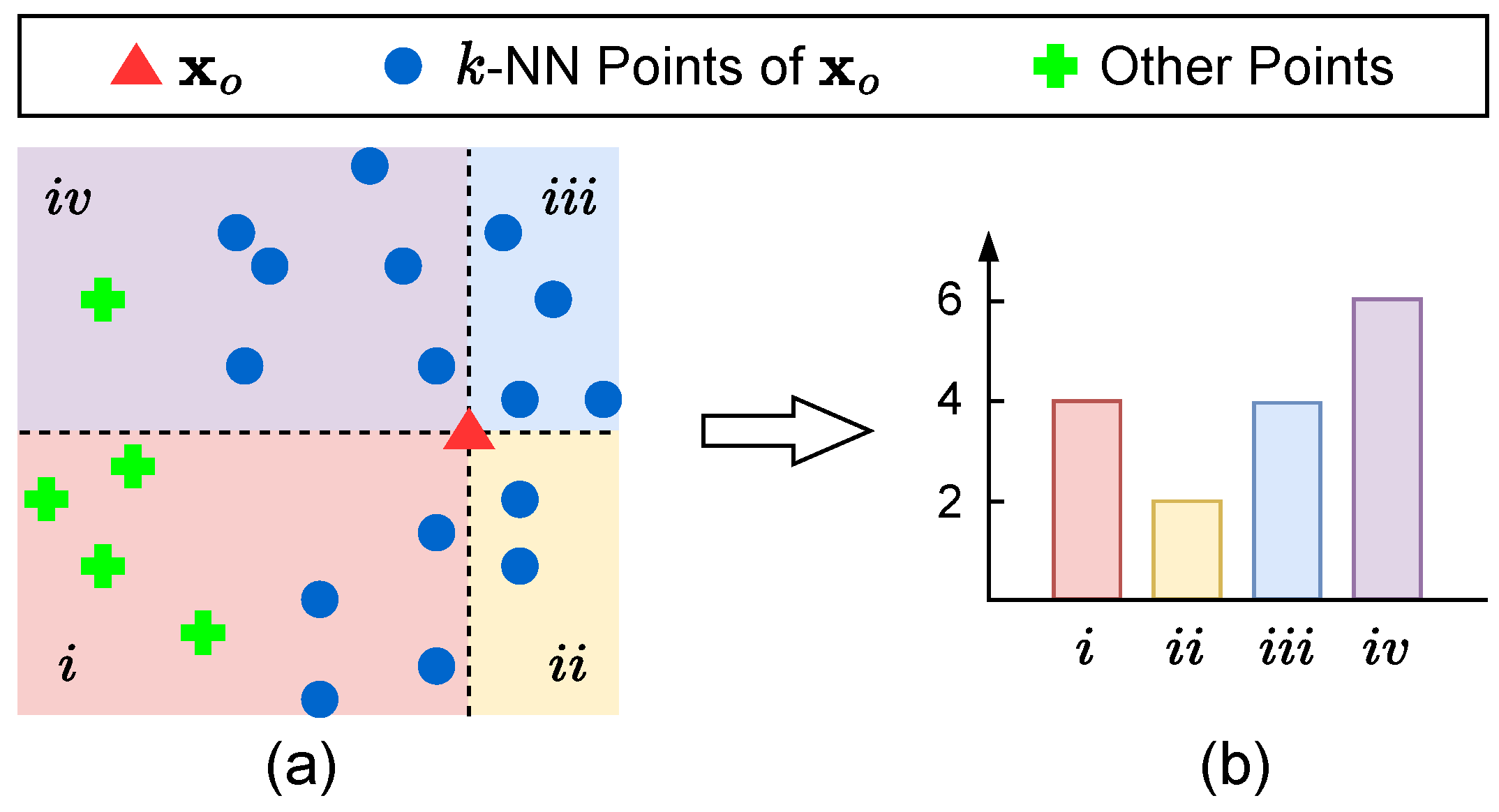
Following the success of general DNN-based point cloud semantic segmentation methods, several recent works have used DNN models for forest point cloud segmentation [7,8,9]. However, general point cloud semantic segmentation and tree point cloud semantic segmentation tasks are essentially different since forest point clouds are much more difficult to annotate and the labelled forest point cloud datasets are much smaller. Therefore, using DNN-based methods alone may not be enough for learning effective representations from forest data. To obtain a better representation for the tree point cloud semantic segmentation task, we proposed a handcrafted feature that characterises the local interaction of points in an explicit manner. Motivated by our observation that stem and foliage points differ by the relative position of their neighbours, we design a histogram-based local feature [70,71] that encodes for each individual point the direction of its neighbour points.

More specifically, given a point coordinate ${\mathbf{x}}_o=[x_o,y_o,z_o]$ and the set of its surrounding points $\mathcal{N}\left({\mathbf{x}}_o\right)$ selected by k-NN search in the 3D space, we first compute the orientation of the vector ${\mathbf{x}}_n-{\mathbf{x}}_o$ for each neighbor point ${\mathbf{x}}_n\in \mathcal{N}\left({\mathbf{x}}_o\right)$ by projecting ${\mathbf{x}}_n-{\mathbf{x}}_o$ onto each of the three 2D planes (i.e., $xOy$, $yOz$, and $zOx$) and computing the three orientation angles corresponding to the three 2D components, i.e.,

$$\begin{array}{cc}\hfill \alpha ({\mathbf{x}}_n-{\mathbf{x}}_o)& \hfill =\varphi (y_n-y_o,x_n-x_o)\hfill \\ \hfill \beta ({\mathbf{x}}_n-{\mathbf{x}}_o)& \hfill =\varphi (z_n-z_o,y_n-y_o)\hfill \\ \hfill \gamma ({\mathbf{x}}_n-{\mathbf{x}}_o)& \hfill =\varphi (x_n-x_o,z_n-z_o)\hfill \end{array}$$

(1)

where the function $\varphi (·,·):\mathbb{R}\times \mathbb{R}\to [0,2\pi )$ computes the angle of the 2D vector given by its two input variables, i.e., when using the $\alpha ({\mathbf{x}}_n-{\mathbf{x}}_o)=\varphi (y_n-y_o,x_n-x_o)$ in (1) as example,

$$\begin{array}{cc}\hfill & r=\sqrt{{(x_n-x_o)}^2+{(y_n-y_o)}^2+ϵ},u=\frac{x_n-x_o}{r},vs.=\frac{y_n-y_o}{r}\hfill \\ \hfill & \varphi (y_n-y_o,x_n-x_o)=\left(𝟙[v>0]·𝟙[u<0]-𝟙[v\le 0]·𝟙[u<0]+1\right)·\pi +\left(2·𝟙[u\ge 0]-1\right)·arcsinv\hfill \end{array}$$

(2)

where the $ϵ$ in r is a small positive value used to avoid zero denominator for u and v, and $𝟙[·]$ is the binary indicator function.

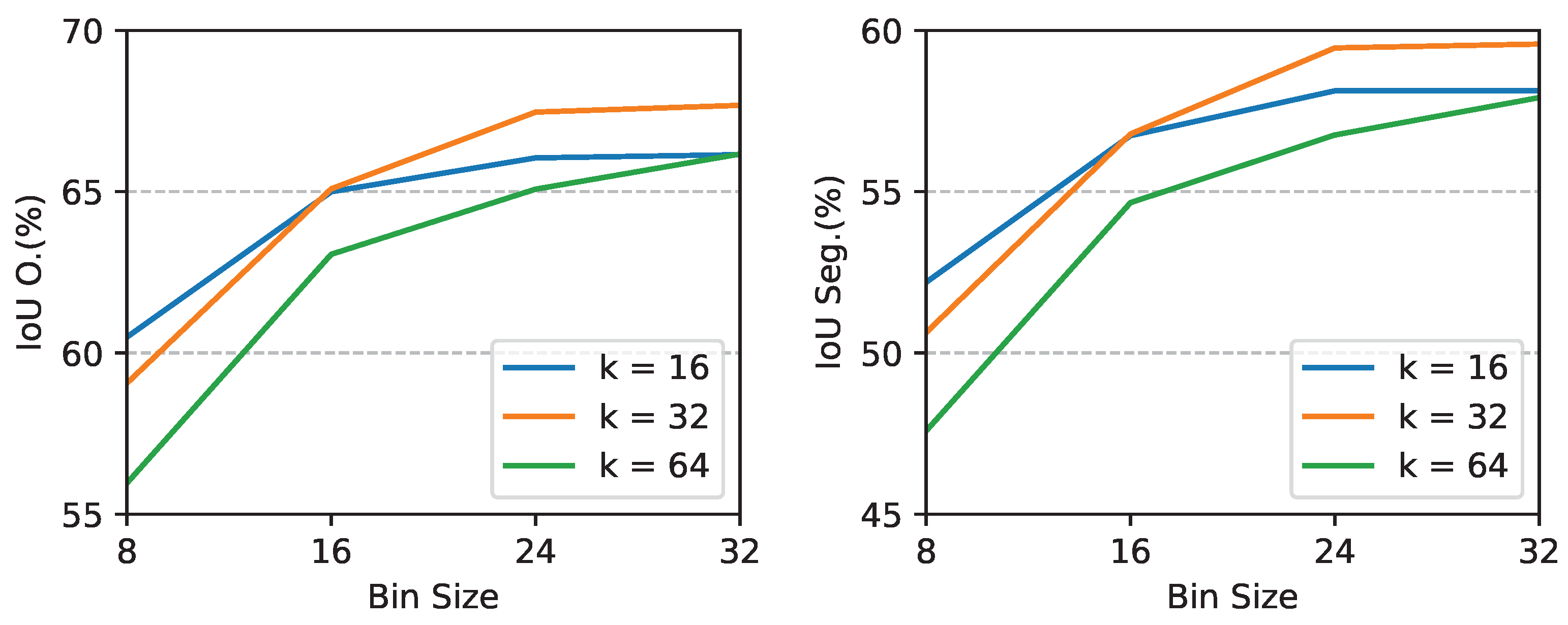
For each of the three angles $\alpha ({\mathbf{x}}_n-{\mathbf{x}}_o)$, $\beta ({\mathbf{x}}_n-{\mathbf{x}}_o)$, and $\gamma ({\mathbf{x}}_n-{\mathbf{x}}_o)$ in (1), we evenly divide the $[0,2\pi )$ interval into B bins and assign the angle to one of the bins. Using the $\alpha ({\mathbf{x}}_n-{\mathbf{x}}_o)$ in (1) for example, the index of the bin to assign the angle is computed as follows,

$$b_{\alpha }({\mathbf{x}}_n-{\mathbf{x}}_o)=⎣\frac{B·\alpha ({\mathbf{x}}_n-{\mathbf{x}}_o)}{2\pi }⎦$$

(3)

where $⎣·⎦$ is the floor operator for numbers. Then we compute the number of points assigned to each bin based on the orientations computed for all ${\mathbf{x}}_n\in \mathcal{N}\left({\mathbf{x}}_o\right)$, i.e.,

$${\displaystyle B_{\alpha }^j\left({\mathbf{x}}_o\right)=\sum _{{\mathbf{x}}_n\in \mathcal{N}\left({\mathbf{x}}_o\right)}𝟙[b_{\alpha }({\mathbf{x}}_n-{\mathbf{x}}_o)=j]}$$

(4)

where $j\in \{0,\dots ,B-1\}$ is the bin index. By the same token, we compute $B_{\beta }^j\left({\mathbf{x}}_o\right)$ and $B_{\gamma }^j\left({\mathbf{x}}_o\right)$ for the other two angles $\beta ({\mathbf{x}}_n-{\mathbf{x}}_o)$ and $\gamma ({\mathbf{x}}_n-{\mathbf{x}}_o)$ in (1).

Finally, our histogram feature $\mathbf{h}\left({\mathbf{x}}_o\right)$ is given by the vector of point numbers across all bins, i.e.,

$$\mathbf{h}\left({\mathbf{x}}_o\right)=[B_{\alpha }^0\left({\mathbf{x}}_o\right),\dots ,B_{\alpha }^{B-1}\left({\mathbf{x}}_o\right),B_{\beta }^0\left({\mathbf{x}}_o\right),\dots ,B_{\beta }^{B-1}\left({\mathbf{x}}_o\right),B_{\gamma }^0\left({\mathbf{x}}_o\right),\dots ,B_{\gamma }^{B-1}\left({\mathbf{x}}_o\right)]$$

(5)

We illustrate our method for computing $\mathbf{h}\left({\mathbf{x}}_o\right)$ in Figure 2.

The histogram feature $\mathbf{h}\left({\mathbf{x}}_o\right)$ only contains the relative position information of points and does not utilise the original 3D point coordinates, while we empirically found it is beneficial to incorporate the point coordinates into our local feature. More specifically, we improve the descriptiveness of our local feature simply by concatenating the coordinate ${\mathbf{x}}_o$ with the corresponding local feature $\mathbf{h}\left({\mathbf{x}}_o\right)$, resulting in a feature dimension of $3B+3$ for each point. For clarity, we denote the improved feature as $\tilde{\mathbf{h}}\left({\mathbf{x}}_o\right)$, i.e.,

$$\tilde{\mathbf{h}}\left({\mathbf{x}}_o\right)=[{\mathbf{x}}_o,\mathbf{h}\left({\mathbf{x}}_o\right)]$$

(6)

When using the handcrafted feature $\tilde{\mathbf{h}}\left({\mathbf{x}}_o\right)$ alone as the segmentation method and not integrating with the DNN-based method, we train a simple multi-layer perceptron (MLP) classifier to predict the segmentation results. In this way, we achieve results on par with popular DNN-based segmentation methods. In Section 3.3, we will combine the advantage of both our handcrafted feature and DNN-based methods for improved performance.

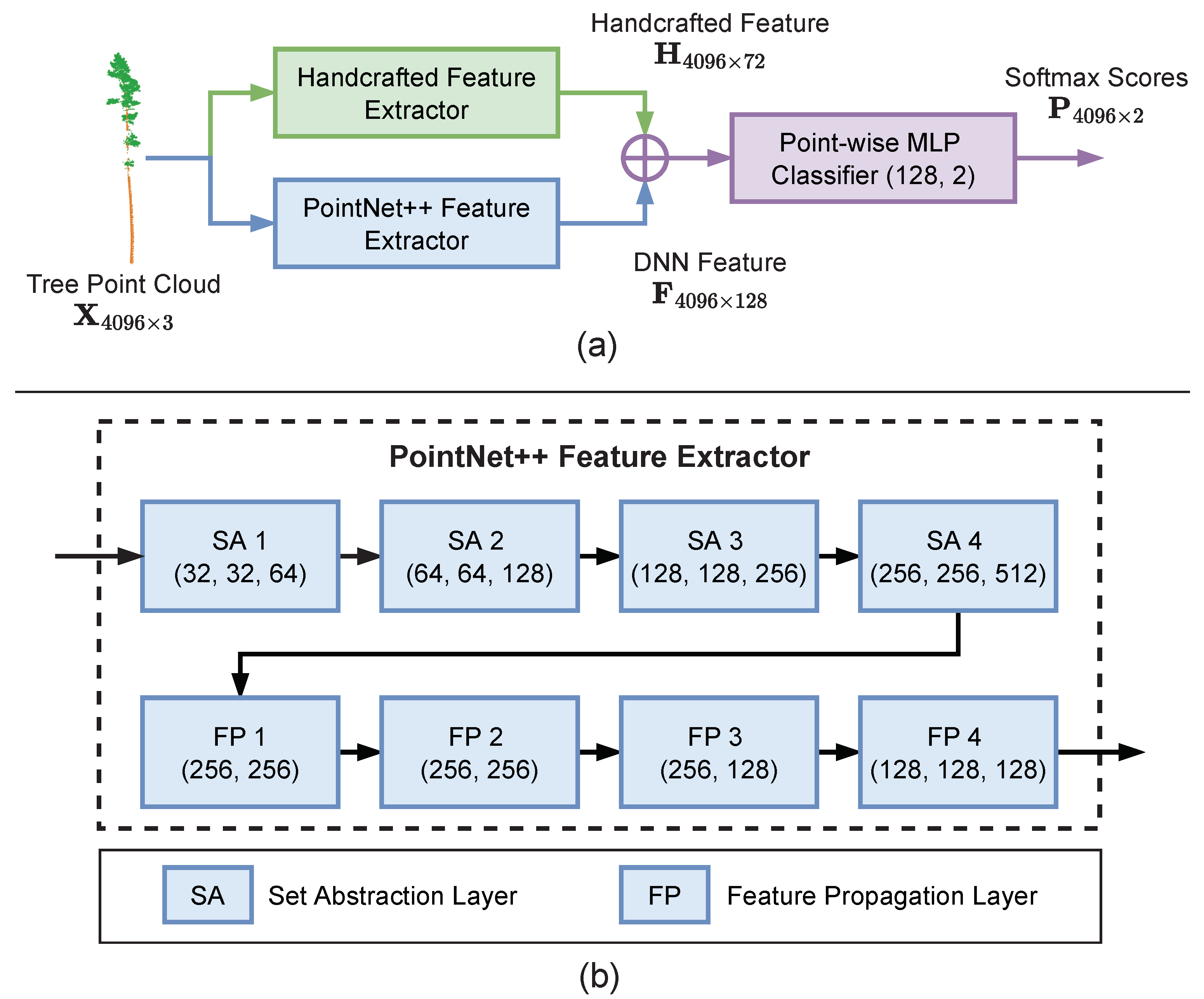
3.3. Point Cloud Segmentation Model

In this subsection, we introduce our backbone semantic segmentation model which we use for all the learning settings involved in this work, i.e., supervised learning, semi-supervised learning, and domain adaptation. Inspired by the success of existing works [23,24,25,26] which integrate DNN with a handcrafted feature for the image recognition and point cloud recognition tasks, we integrate our handcrafted local feature with a DNN model for the point cloud semantic segmentation task. In this way, our backbone point cloud semantic segmentation model can combine the benefits of both types of methods.

For the DNN component in our point cloud semantic segmentation model, we use the popular PointNet++ [18] model. In the encoder network of PointNet++, the Farthest Point Sample algorithm [72] is used to divide the points into local groups and several set abstraction modules are used to gradually capture semantics from a larger spatial extent. Then in the decoder, an interpolation strategy based on the spatial distance between point coordinates is used to propagate features from the semantically rich sampled points to all the original points.

To integrate our handcrafted feature with the PointNet++ model, for each individual point, we concatenate our handcrafted feature vector with the output feature vector of the last feature propagation layer in the decoder component of PointNet++. We illustrate our backbone point cloud semantic segmentation model in Figure 3.

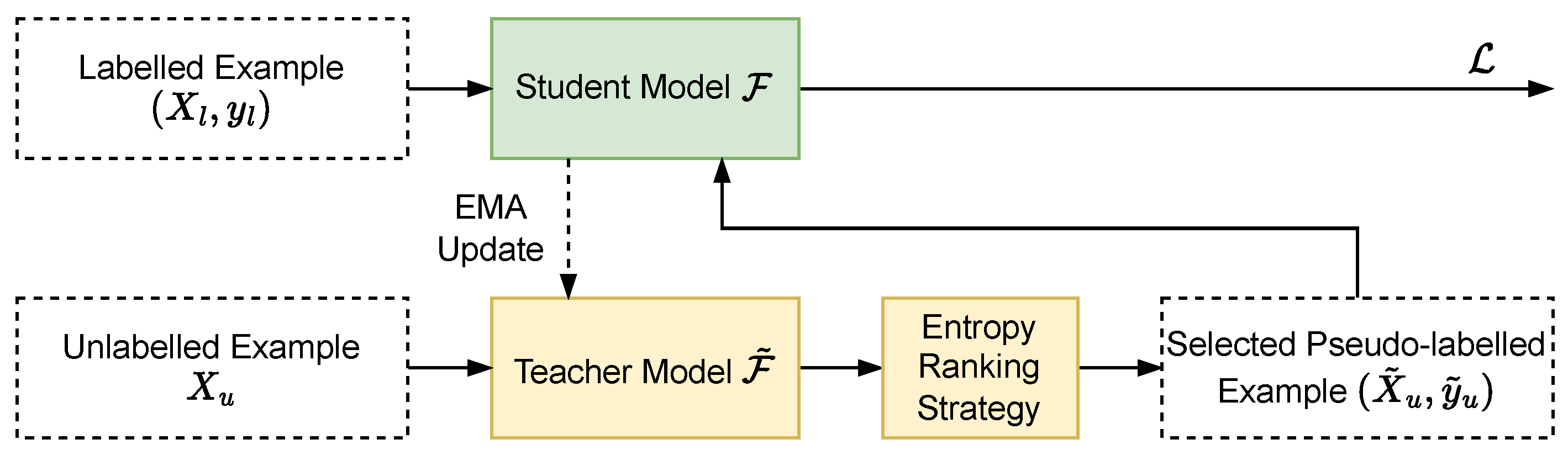
3.4. Learning Framework for Semi-Supervised Point Cloud Semantic Segmentation

To address the issue of limited labelled data for training the semantic segmentation model, we utilise unlabelled examples for training the model by employing semi-supervised learning. We propose a learning framework based on pseudo-labelling and model ensembling to utilise the unlabelled training data.

Formally, we denote the labelled point cloud dataset as ${\mathcal{X}}^l={\left\{({\mathbf{X}}_i^l,{\mathbf{Y}}_i^l)\right\}}_{i=1}^{N_l}$, where ${\mathbf{X}}_i^l\in {\mathbb{R}}^{P_i\times 3}$ is a labelled example with $P_i$ being the number of points in ${\mathbf{X}}_i^l$ and ${\mathbf{Y}}_i^l\in {\{1,\dots ,K\}}^{P_i}$ is the set of semantic labels corresponding to each point in ${\mathbf{X}}_i^l$ with K being the total number of semantic classes.

Inspired by the model ensembling and distillation strategy [52], in our learning framework, we employ two point cloud semantic segmentation models (i.e., one student model and one teacher model) with an identical architecture. During the training process, we first use the teacher model to produce pseudo-labels ${\widehat{\mathbf{Y}}}_i^u$ for each unlabelled example ${\mathbf{X}}_i^u$ and train the student model on both the labelled examples and the pseudo-labelled examples, then update the variables in the teacher model by taking Exponential Moving Average (EMA) of the variables in the student model. More specifically, we denote the student model function as $\mathcal{F}(·,{\Theta }_{\mathcal{F}}):{\mathbb{R}}^{N\times 3}\to {\mathbb{R}}^{N\times K}$, where the output is the prediction probability matrix over all points and semantic classes and ${\Theta }_{\mathcal{F}}=\left\{{\theta }_{\mathcal{F}}^j\right\}$ is the set of model variables with j being the layer index of DNN model. Similarly, we use $\tilde{\mathcal{F}}(·,{\Theta }_{\tilde{\mathcal{F}}})$ to denote the teacher model function. We also use the indices p and k to indicate the p-th point and the k-th semantic class in the prediction probability matrix, respectively. Then we formulate our pseudo-labelling strategy, overall training loss function, and EMA update strategy for the teacher model as Equations (7)–(9) as follows,

$$\begin{array}{cc}\hfill {\widehat{y}}_{i,p}^u& \hfill =\underset{k\in \{1,\dots ,K\}}{arg\; max}{\left[\tilde{\mathcal{F}}({\mathbf{X}}_i^u;{\Theta }_{\tilde{\mathcal{F}}})\right]}_{p,k},\forall i,p\hfill \end{array}$$

(7)

$$\begin{array}{cc}\hfill \mathcal{L}& \hfill =\frac{1}{N_l}\sum _{i=1}^{N_l}{\mathcal{L}}_{CE}(\mathcal{F}({\mathbf{X}}_i^l;{\Theta }_{\mathcal{F}}),{\mathbf{Y}}_i^l)+w·\frac{1}{N_u}\sum _{i=1}^{N_u}{\mathcal{L}}_{CE}(\mathcal{F}({\mathbf{X}}_i^u;{\Theta }_{\mathcal{F}}),{\widehat{\mathbf{Y}}}_i^u)\hfill \end{array}$$

(8)

$$\begin{array}{cc}\hfill {\theta }_{\tilde{\mathcal{F}}}^j& \hfill \leftarrow \eta {\theta }_{\tilde{\mathcal{F}}}^j+(1-\eta ){\theta }_{\mathcal{F}}^j,\forall j\hfill \end{array}$$

(9)

where ${\widehat{y}}_{i,p}^u\in \mathbb{R}$ is p-th element in the pseudo-label vector ${\widehat{\mathbf{Y}}}_i^u$ (i.e., the pseudo-label predicted by the teacher model for the p-th point of ${\mathbf{X}}_i^u$), ${\mathcal{L}}_{CE}(·,·)$ denotes the Cross-Entropy loss function, w is a weight factor for balancing the two loss terms, and $\eta$ is a constant factor called momentum that is set to $0.97$ in our experiments.

The main issue with the pseudo-labelling strategy is the quality of pseudo-labelled examples as the lack of variety can harm model performance. Inspired by [73], we propose a pseudo-label selection strategy based on the entropy ranking of the individual points to select the pseudo-labelled points in each point cloud that are beneficial for training the segmentation model. More specifically, for each ${\mathbf{X}}_i^u$, we compute the entropy of each individual point and select the $80\%$ points with higher entropy as the pseudo-labelled points. Therefore, we denote the updated $({\mathbf{X}}_i^u,{\widehat{\mathbf{Y}}}_i^u)$ with only the selected points and their corresponding pseudo-labels as $({\tilde{\mathbf{X}}}_i^u,{\tilde{\mathbf{Y}}}_i^u)$. In this way, we are selecting the hard examples which are better for the variety of the training dataset. We illustrate our complete learning framework for semi-supervised and cross-dataset point cloud semantic segmentation in Figure 4.

3.5. Extending Semi-Supervised Learning Framework to Domain Adaptation

In practice, aside from the shortage in labelled training data, we often face situations where the training data and test data are collected from different scenes and do not follow the same data distribution. For example, in the forest inventory scenario, the training and test data can be of different tree species, or collected using different types of LiDAR devices or from different sites. In learning theory, this is known as the “domain adaptation” or cross-dataset generalisation problem, and the data distributions of the training and test data are called the source domain and the target domain, respectively. The domain adaptation problem is usually tackled by exploiting the training data from the target domain, while we tackle the more challenging setting of unsupervised domain adaptation where the target training data are unlabelled. Using unlabelled target training data is more advantageous than using labelled training data in real-world applications since it saves time and the cost of annotation.

For the cross-dataset point cloud semantic segmentation task, we can extend our semi-supervised learning framework in Section 3.4 to the domain adaptation setting by simply replacing the training datasets, i.e., we replace the labelled dataset ${\mathcal{X}}^l$ and unlabelled dataset ${\mathcal{X}}^u$ with the labelled source dataset ${\mathcal{X}}^s={\left\{({\mathbf{X}}_i^s,{\mathbf{Y}}_i^s)\right\}}_{i=1}^{N_s}$ and the unlabelled target dataset ${\mathcal{X}}^t={\left\{{\mathbf{X}}_i^t\right\}}_{i=1}^{N_t}$, respectively. Different from the ${\mathcal{X}}^l$ and ${\mathcal{X}}^u$ in semi-supervised learning which are assumed to be drawn from the same data distribution, the ${\mathcal{X}}^s$ and ${\mathcal{X}}^t$ in domain adaptation are drawn from different data distributions.

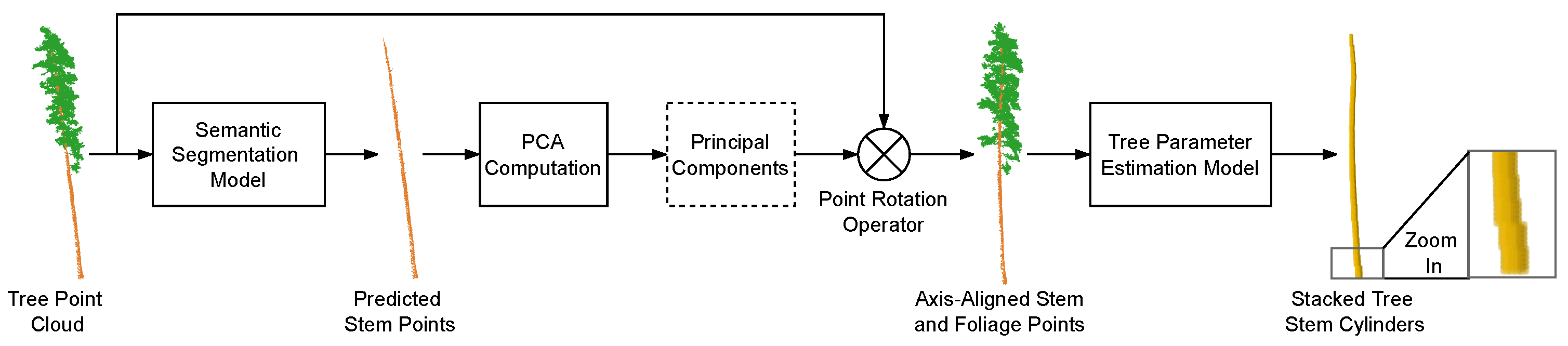
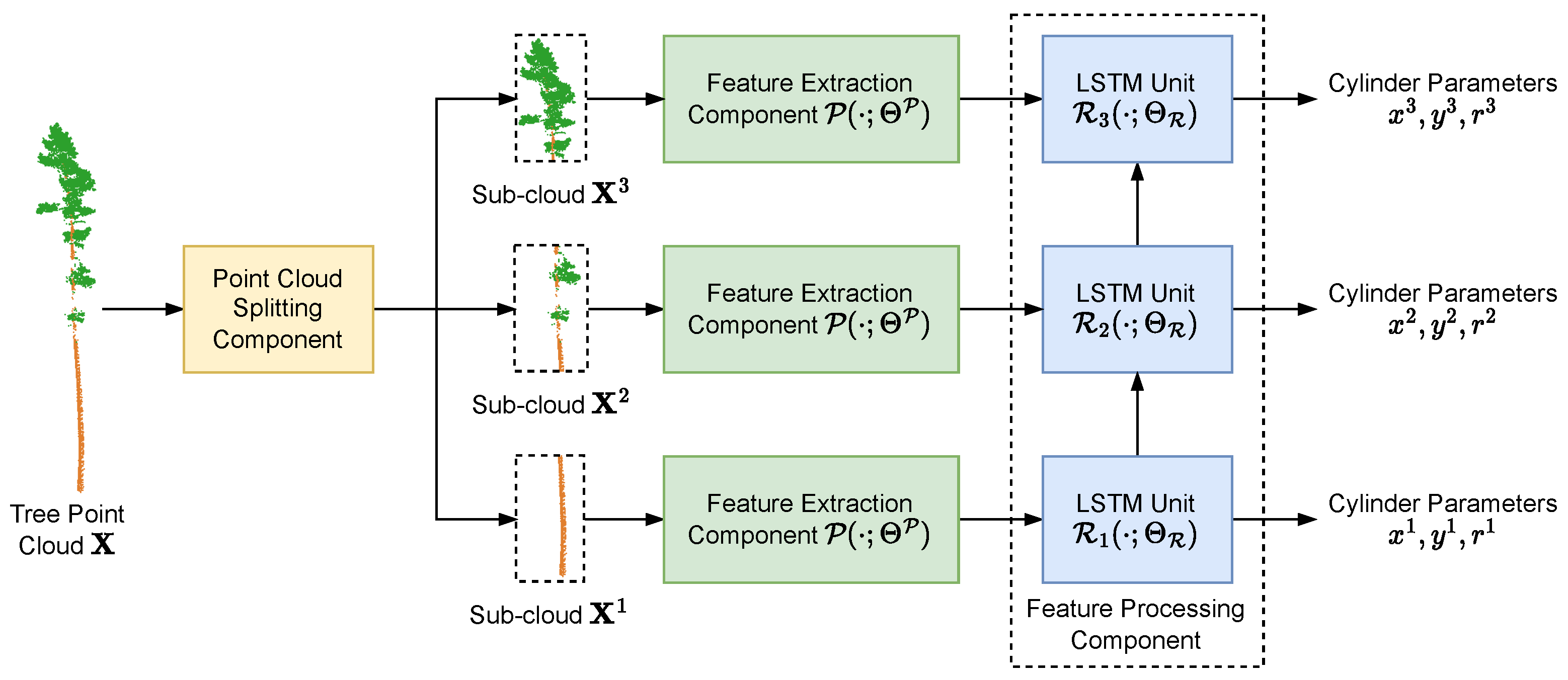
3.6. Tree Parameter Estimation Model

Existing works in tree parameter estimation mainly fit a parametric model to characterise the tree stem geometry for each tree point cloud individually. In contrast to the existing works, we propose a data-driven method for tree parameter estimation based on DNN to predict the cylindrical parameters of the tree stem [10] while being able to learn from the variety of data for improved robustness and adaptability to geometric variations across different individual trees.

In particular, our DNN tree parameter estimation method consists of three components, splitting the point cloud into sub-clouds based on height, extracting features from each sub-cloud, and feature processing. Each individual tree point cloud ${\mathbf{X}}_i$ is first passed through the point cloud division component, where we first divide the height range from 0 to 50 m into M segments, then group the subset of points (both stem and foliage points) fallen into the m-th height segment as the tree point cloud segment ${\mathbf{X}}_i^m$. Here we are overloading the denotation by using the superscript of ${\mathbf{X}}_i$ to indicate the tree segment index instead of the dataset as in Section 3.4 and Section 3.5. Then in the segment-wise feature extraction component, we use a PointNet [17] feature extractor on each tree point cloud segment individually to extract segment-wise semantics, while the PointNet feature extractor for each individual tree segment has a shared set of model parameters. The features extracted across the segments of an individual tree naturally form a sequence. Finally, in the feature processing component, we employ a Long Short-Term Memory (LSTM) [74] model to process the sequential features across all the tree segments ${\left\{{\mathbf{X}}_i^m\right\}}_{m=1}^M$ and predict the tree parameters for each segment, i.e., the planar center coordinates ${\left\{(x_i^m,y_i^m)\right\}}_{m=1}^M$ of the stem segments along the X- and Y- axes and the stem segment radii ${\left\{r_i^s\right\}}_{m=1}^M$. For the ease of denotation, we write the tree parameters $x_i^m$, $y_i^m$, and $r_i^m$ collectively as ${\mathbf{v}}_i^m$.

Inspired by the recent works in point cloud object detection [75,76,77], for estimating the coordinates $x_i^m$ and $y_i^m$, we let our tree parameter estimation model predict the residual between $(x_i^m,y_i^m)$ and the point centroid $({\overline{x}}_i^m,{\overline{y}}_i^m)$ of each point cloud segment instead of directly predict $(x_i^m,y_i^m)$. When computing each centroid $({\overline{x}}_i^m,{\overline{y}}_i^m)$, we first compute the initial centroid ${\overline{x}}_{o,i}^m,{\overline{y}}_{o,i}^m$ by simply averaging the X- and Y-coordinates of the points within the corresponding point cloud segment, then we evenly divide the $xOy$-plane centred on ${\overline{x}}_{o,i}^m,{\overline{y}}_{o,i}^m$ into 16 directional bins. Finally, we compute $({\overline{x}}_i^m,{\overline{y}}_i^m)$ by randomly sampling a maximum of 4 points from each directional bin and taking the average on the X- and Y-coordinates of the sampled points. By refining ${\overline{x}}_{o,i}^m,{\overline{y}}_{o,i}^m$ into ${\overline{x}}_i^m,{\overline{y}}_i^m$ in this way, we can reduce the errors of the initial centroids caused by sampling bias during LiDAR scanning. Therefore, we formulate our total loss function across all the tree segments as follows,

$${\mathcal{L}}_{param}=\frac{1}{NM}\sum _{i=1}^N\sum _{m=1}^M{\mathcal{L}}_{huber}\left({\mathcal{R}}_m\circ \mathcal{P}({\mathbf{X}}_i^m;{\Theta }_{\mathcal{P}},{\Theta }_{\mathcal{R}}),{\mathbf{v}}_i^m-{\mathbf{c}}_i^m\right)$$

(10)

where ${\mathbf{c}}_i^m=[{\overline{x}}_i^m,{\overline{y}}_i^m,0]$ is the centroid coordinate vector extended by an additional zero to match the dimension of ${\mathbf{v}}_i^m$, N is the number of tree point clouds in the dataset, ${\mathcal{L}}_{huber}(·,·)$ is the Huber loss function with the $\delta$ coefficient set to 0.01, $\mathcal{P}(·;{\Theta }_{\mathcal{P}})$ and ${\mathcal{R}}_m(·;{\Theta }_{\mathcal{R}})$ are the model functions of the PointNet feature extraction component and the LSTM feature processing component, respectively. $\mathcal{P}(·;{\Theta }_{\mathcal{P}})$ maps each point cloud segment into a D-dimensional feature vector while each ${\mathcal{R}}_m(·;{\Theta }_{\mathcal{R}})$ maps its input features into the tree parameters. We illustrate our tree parameter estimation model in Figure 5.

In addition, we also use a data augmentation strategy during the training process to improve the robustness of our tree parameter estimation method. For each ${\mathbf{X}}_i$, we apply a rotation with random angle along the vertical Z-axis to the whole point cloud ${\mathbf{X}}_i$ while we also apply the same rotation to the $x_i^m$ and $y_i^m$ coordinates in each ${\mathbf{v}}_i^m$ across all m. We denote this example-specific rotation operator as ${\phi }_i(·)$. Therefore, by incorporating our data augmentation strategy into the training process, our loss function in (10) is updated as,

$${\mathcal{L}}_{param}=\frac{1}{NM}\sum _{i=1}^N\sum _{m=1}^M{\mathcal{L}}_{huber}\left({\mathcal{R}}_m\circ \mathcal{P}({\phi }_i\left({\mathbf{X}}_i^m\right);{\Theta }_{\mathcal{P}},{\Theta }_{\mathcal{R}}),{\phi }_i({\mathbf{v}}_i^m-{\mathbf{c}}_i^m)\right)$$

(11)

Note in (11) that our data transform ${\phi }_i(·)$ works differently for ${\mathbf{X}}_i^m$ and ${\mathbf{v}}_i^m$ since the Z-coordinates in ${\mathbf{X}}_i^m$ are replaced by the radius in ${\mathbf{v}}_i^m$, while we write ${\phi }_i(·)$ as the same type of transform for both ${\mathbf{X}}_i$ and ${\mathbf{v}}_i$ for the ease of denotation. We only use random rotation for ${\phi }_i(·)$ during the training process and we use the identity operator for ${\phi }_i(·)$ during testing.

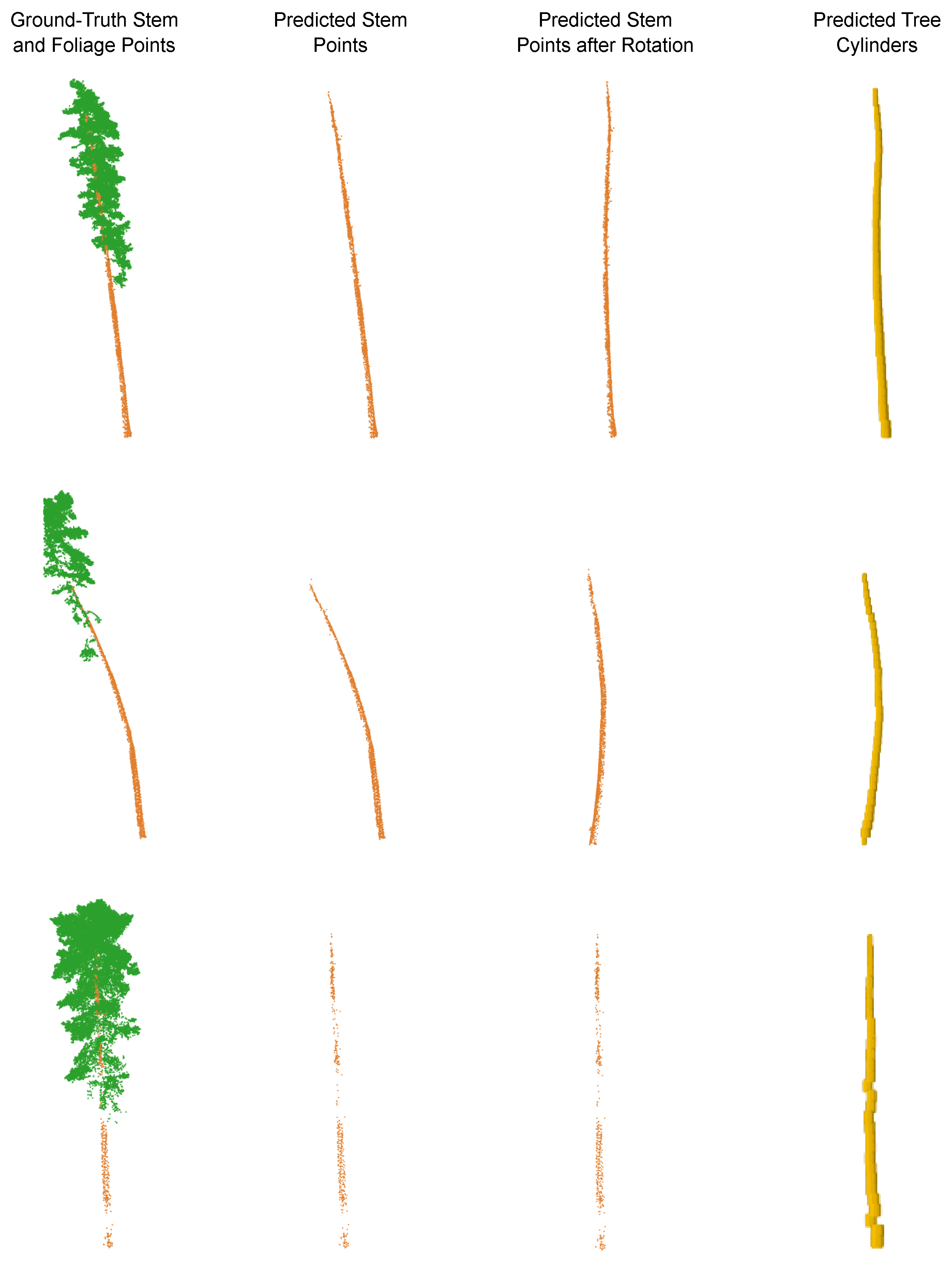
In addition, we also propose a simple tree point cloud semantic segmentation model which is induced from our tree parameter estimation model. Intuitively, for each cylinder segment characterised by the parametric tree model, we classify a point within the corresponding point cloud segment as a stem if the point falls within the interior of the cylinder segment, otherwise we classify the point as foliage. More specifically, given a tree stem segment with parameters $(x_i^m,y_i^m,r_i^m)$ and a point $(x,y)$ from the corresponding point cloud segment, we classify $(x,y)$ as stem if it falls within a distance threshold to $(x_i^m,y_i^m)$, i.e.,

$${(x-x_i^m)}^2+{(y-y_i^m)}^2\le {\left(r_i^m(1+\zeta )\right)}^2$$

(12)

where $\zeta$ is a positive coefficient we use to improve the robustness of the model. We name this induced tree point cloud semantic segmentation model the cylinder segmentation model. Following the procedure of our tree parameter estimation method, we use the PCA-transformed points in our cylinder segmentation.

4. Experimental Results and Discussion

4.1. Datasets

Experiments were performed using point cloud data taken from a variety of forest types using both airborne and terrestrial laser scanning. Airborne datasets were captured using a Reigl VUX-1 scanner mounted to a helicopter that flew approximately 60–90 m above the forest canopy, capturing data at approximately 300 to 700 points per ${\mathrm{m}}^2$. Ground-based datasets were captured using a mobile back-pack mounted Emesent Hovermap scanner, capturing at approximately 8000 points per ${\mathrm{m}}^2$. Each forest scan was split into per-tree point clouds based on the method described in [10], for individual tree detection. Four different datasets of trees were compiled:

• Tumut: Mature Radiata pine trees from a forest outside Tumut, NSW, Australia captured using airborne scanning.
• HQP: Caribbean Pine spp. trees from a commercial plantation in Queensland, Australia, captured using mobile ground-based scanning.
• ct03: Commercial plantation in Tasmania, Australia, captured using mobile ground-based scanning
• DogPark: Recreational forest (various species) in Rotorua, New Zealand, captured using mobile ground-based scanning.

Ground-truth per-point annotation/labelling: Each point in each per-tree point cloud was manually labelled as being either part of the main tree stem (including stem splits and forks) or tree foliage, using the selection tools in the software package Meshlab (Version 2016.12, P. Cignoni, https://www.meshlab.net/ (accessed on 1 January 2023)). The resulting ground truth labels were used for training and validation in the experiments described below.

We use the four datasets for both the point cloud semantic segmentation task and the tree parameter estimation task in our experiments. The trees in the four datasets have significant intra-dataset variations in geometry which makes both semantic segmentation and tree parameter estimation challenging, while the trees also have clear inter-dataset differences caused by the different laser scanning patterns and different tree species which puts an additional challenge to cross-dataset semantic segmentation. In the cross-dataset point cloud semantic segmentation task, our four datasets lead to 12 different cross-dataset scenarios. We visualise some tree point cloud examples from each dataset in Figure 6.

We split each of the four datasets into a training set and a validation set. The numbers of training and validation examples in each dataset are given in

Table 1. The number of training and validation tree point cloud examples in each of our four datasets.

Dataset	Tumut	HQP	ct03	DogPark
Training	60	86	17	30
Validation	30	40	10	20

.

For the semi-supervised and cross-dataset semantic segmentation tasks, we reorganise the training sets in the following ways. In the semi-supervised learning setting, for each of the four datasets, we select 5 training examples as the labelled examples and use the rest of the training examples as the unlabelled examples. In the domain adaptation setting, we use all the labelled examples in the source training set while we discard the labels of the target training examples and use them as unlabelled examples.

4.2. Experimental Setup

4.2.1. Point Cloud Semantic Segmentation

(i) 

Data Pre-processing and Data Augmentation

We normalise each point cloud example into the unit 3D sphere as following the standard practice in [17]. For each iteration during both the training and testing processes, we randomly sample 4096 points from each point cloud. During the training process, we also apply data augmentation to each training point cloud example by using random rotation along the vertical Z-axis and adding a random noise variable to each of the three coordinates of each individual point. We sample each random noise variable from the 1D Gaussian distribution with a mean of 0 and a standard deviation of $4\times {10}^{-4}$.

(ii) 

Model Configuration

We jointly use a PointNet++ [18] semantic segmentation network and our handcrafted local feature in our backbone model for point cloud semantic segmentation. For PointNet++, we use the original network architecture while we set the ball query radius to 0.5 times the default value at each set abstraction layer. For our handcrafted feature, we set the neighbourhood size k to 16 for the k-NN query and set the number of bins b to 24. We empirically found these hyper-parameters yield the best results.

(iii) 

Experimental Details

We use the Adam optimiser [78] with a momentum of 0.9 when training each semantic segmentation model. We train each model for 5000 iterations with the constant learning rate of $1\times e^{-3}$ and we use a batch size of 10. In the semi-supervised learning and domain adaptation settings which involve the additional unsupervised learning objective, the weight w on the unsupervised loss term is kept at 0 over the first 4000 training iterations and linearly increases to 1 between the 4000th and 4100th iterations. Our method is implemented in Tensorflow and trained on a work station with one NVIDIA GTX 1080Ti GPU.

(iv) 

Baselines

We compare the performance of our backbone model with the popular DNN models PointNet [17] and PointNet++ [18] as well as the segmentation method which only uses our handcrafted feature. In the method based solely on our handcrafted feature, we use a point-wise MLP with a single hidden layer of 128 channels. We also integrate our handcrafted feature with the PointNet semantic segmentation network in a similar fashion to our backbone model using PointNet++ as an additional baseline.

(v) 

Evaluation Criterion

We use two different types of Intersection-over-Union (IoU) metrics as our performance indicators, i.e., the overall IoU and the average IoU over per-height segments. For the overall IoU, we simply compute the IoU over the stem points of each entire tree point cloud. For the average IoU over height segments, we first divide the stem part of the point cloud by height segment in the same fashion as in Section 3.6 and compute the IoU for each segment individually, then we average the IoU over the non-empty segments that each contains at least one stem point. We observed that in some datasets capture using terrestrial LiDAR devices (e.g., HQP), the stem points are plenty and dense towards the bottom while few and sparse towards the tip. The issue with this point sampling bias is that the amount of stem points near the bottom is more than necessary for tree parameter estimation while the stem points near the tip are insufficient and makes tree parameter estimation difficult. Therefore, we use the average IoU over height segments as a fairer performance metric to indicate how each segmentation method performs across different height segments. For ease of narration we write our overall IoU and average IoU over height segments as IoU O. and IoU Seg., respectively.

During the testing process, for each validation point cloud example, we repetitively sample points from the point cloud until each point is sampled 15 times on average, which produces multiple down-sampled point clouds (4096 points in each) of the original one. For example, given a point cloud with 10,000 points, we sample 4096 points each time 37 times, producing 37 down-sampled point clouds while the average number of sampling per point is 15.16. After sampling, we feed each of the multiple down-sampled point clouds into the trained segmentation model for inference which produces an average of 15 segmentation predictions per point. To aggregate the different predictions across the down-sampled point clouds, we use a simple voting strategy to determine the semantic class for each individual point, i.e., the point is determined to be a stemmed point if no less than 50% of the predictions on this point are stem, otherwise the point is determined to be a foliage point. By our voting strategy, we not only can obtain the segmentation predictions on all the points in each validation point cloud example, but also can improve the segmentation performance.

Additionally, for each of our four datasets, we create three different training and validation splits with differently grouped point cloud examples while the numbers of training and validation examples are the same as in Table 1, and we average the testing IoU over the three different validation sets for fair comparison.

4.2.2. Tree Parameter Estimation

(i) 

Tree Parameter Generation

We employ the cylinder model fitting method proposed by Windrim et al. [10] to generate the cylinder parameters $x_i$, $y_i$, and $r_i$ for each height segment in each tree point cloud. In particular, for each tree, we first use the stem points predicted by our semantic segmentation model (PointNet++ with the handcrafted feature) to perform Principle Component Analysis (PCA), then use the PCA components of the predicted stem points to transform the ground-truth stem points. Finally, we apply the fitting method in [10] to the PCA-transformed ground-truth stem points. Note that for each tree there are height segments above the tree tip which results in empty tree point cloud segments without points, and we set the $x_i$, $y_i$, and $r_i$ to zeros for these empty segments.

(ii) 

Data Pre-processing and Data Augmentation

We follow the same data pre-processing scheme and data augmentation strategy as we use for the point cloud semantic segmentation task, except that we do not normalise the point clouds for the tree parameter estimation task and we rotate both the point cloud and the segment-wise stem parameters along the vertical Z-axis when augmenting each training example as mentioned in Section 3.6.

(iii) 

Model Configuration

In our tree parameter estimation model, we use the encoder network of the PointNet [17] semantic segmentation model (i.e., from the input to the pooling layer of the PointNet) as the feature extraction component and employ a Bidirectional LSTM [79] as the feature processing component which can better exploit the sequential property of the tree stem parameters than the original LSTM [74]. We use the original PointNet encoder network and we set the number of channels in each LSTM unit to 128. For our cylinder segmentation model in Section 3.6, we select the $\zeta$ coefficient from $\{0.5,0.6,0.7,0.8\}$ depending on the dataset.

(iv) 

Experimental Details

The experimental details for training our tree parameter estimation model are the same as those for training our point cloud semantic segmentation model, except that we train the tree parameter estimation model for 2000 iterations while the learning rate starts at $\mathbf{2}\times {\mathbf{10}}^{-\mathbf{3}}$ and decays to $\mathbf{2}\times {\mathbf{10}}^{-\mathbf{4}}$ at the 1600-th iteration.

(v) 

Evaluation Criterion

We use both the testing IoU of our cylinder segmentation model and the ${\ell }_2$ regression error of the predicted cylinder centres to evaluate our tree parameter estimation method, while we evaluate our method in the supervised learning setting. For the evaluation using IoU, we compute the semantic predictions of all points for each validation example and compare the segmentation result against the supervised semantic segmentation methods. Following our evaluation criterion for the semantic segmentation, we use the same three training and validation splits for each of the four datasets and average the testing results over the three validation sets, while we also use both the IoU O. and IoU Seg. to evaluate performance.

4.3. Results of Semantic Segmentation Experiments

4.3.1. Supervised Semantic Segmentation

We present the supervised semantic segmentation results of our method and the baseline methods in

Table 2. The overall IoU (IoU O.) and average IoU over height segments (IoU Seg.) of the point cloud semantic segmentation methods under the supervised setting. We report the average results and standard deviations over the three different training and validation splits for each dataset and we highlight (in bold) the best result across different methods on each dataset.

	Method	Tumut	HQP	ct03	DogPark	Avg.
IoU O.	PN	$58.35\pm 2.49$	$86.77\pm 6.72$	$78.51\pm 2.19$	$77.48\pm 2.58$	$75.28$
	PN2	$81.08\pm 1.45$	$\mathbf{88.82}\pm \mathbf{7.99}$	$86.68\pm 2.66$	$89.22\pm 1.24$	$86.45$
	H (Ours)	$67.47\pm 3.05$	$87.11\pm 7.04$	$84.46\pm 1.27$	$89.99\pm 0.77$	$82.26$
	PN + H (Ours)	$75.81\pm 2.57$	$88.68\pm 7.75$	$85.25\pm 1.47$	$\mathbf{91.77}\pm \mathbf{0.07}$	$85.38$
	PN2 + H (Ours)	$\mathbf{81.96}\pm \mathbf{2.02}$	$88.81\pm 7.74$	$\mathbf{87.03}\pm \mathbf{2.31}$	$90.79\pm 1.89$	$\mathbf{87.15}$
IoU Seg.	PN	$53.87\pm 1.34$	$73.86\pm 3.63$	$61.42\pm 2.87$	$55.64\pm 4.84$	$61.20$
	PN2	$75.16\pm 1.61$	$73.57\pm 5.25$	$73.49\pm 2.76$	$77.27\pm 0.93$	$74.87$
	H (Ours)	$59.46\pm 1.93$	$69.52\pm 3.71$	$63.36\pm 1.76$	$74.34\pm 2.22$	$66.67$
	PN + H (Ours)	$69.00\pm 1.55$	$\mathbf{74.93}\pm \mathbf{6.58}$	$69.11\pm 1.61$	$77.83\pm 1.15$	$72.72$
	PN2 + H (Ours)	$\mathbf{76.44}\pm \mathbf{1.47}$	$73.81\pm 4.48$	$\mathbf{73.92}\pm \mathbf{2.36}$	$\mathbf{78.86}\pm \mathbf{1.21}$	$\mathbf{75.76}$

. The four datasets Tumut, HQP, ct03, and DogPark are denoted as T, H, C, and D, respectively. We use PN, PN2, and H to denote PointNet, PointNet++, and our handcrafted feature, respectively, and use PN + H and PN2 + H to denote PointNet with handcrafted feature and PointNet++ with handcrafted feature, respectively.

Our handcrafted feature when used in combination with a simple MLP with one hidden layer, achieves the average IoU O. and IoU Seg. of $82.26\%$ and $66.67\%$, respectively, which surpass the PointNet baseline by $6.98\%$ and $5.47\%$, respectively. This demonstrates the effectiveness of our handcrafted feature method. By combining our handcrafted feature with PointNet++, we achieve the best average IoU O. and IoU Seg. of $87.15\%$ and $75.76\%$, which improve the PointNet++ baseline by $0.70\%$ and $0.89\%$, respectively. Furthermore, when combining our handcrafted feature with PointNet as an alternative to our baseline segmentation model, we achieve an average IoU O. and IoU Seg. of $85.38\%$ and $72.72\%$, which improves our handcrafted feature baseline by $3.12\%$ and $6.05\%$, respectively. These results indicate it is beneficial to jointly utilise DNN and our handcrafted feature for the tree point cloud semantic segmentation task, while our handcrafted feature method is generic and can be combined with different DNN point cloud semantic segmentation models.

4.3.2. Semi-Supervised Semantic Segmentation

We further evaluate how our semi-supervised learning and domain adaptation framework for point cloud semantic segmentation performs under the semi-supervised learning setting. We compare our semi-supervised learning method with the supervised baselines which are only trained on 5 labelled training examples for each dataset and each split. The results are presented in

Table 3. The overall IoU (IoU O.) and average IoU over height segments (IoU Seg.) of the point cloud semantic segmentation methods under the semi-supervised learning setting, where each training set has only 5 labelled examples. We compare the results of our semi-supervised methods (denoted as Semi.) using two different backbone models with the supervised baselines (denoted as Sup.). We report the average results and standard deviations over the three different training and validation splits for each dataset and we highlight (in bold) the best result across different methods on each dataset.

	Method	Tumut	HQP	ct03	DogPark	Avg.
IoU O.	Sup. (PN)	$54.34\pm 3.72$	$82.20\pm 5.83$	$74.71\pm 2.33$	$70.26\pm 2.00$	$70.37$
	Sup. (H)	$65.90\pm 2.48$	$86.41\pm 6.71$	$82.27\pm 0.32$	$86.70\pm 2.58$	$80.32$
	Sup. (PN + H)	$68.91\pm 1.17$	$86.92\pm 7.56$	$83.62\pm 1.60$	$86.52\pm 1.84$	$81.49$
	Sup. (PN2)	$77.83\pm 3.14$	$87.65\pm 6.76$	$85.56\pm 3.96$	$85.75\pm 1.66$	$84.20$
	Sup. (PN2 + H)	$78.04\pm 3.64$	$88.41\pm 7.49$	$86.66\pm 2.83$	$87.80\pm 2.95$	$85.23$
	Semi. (PN2)	$78.50\pm 3.24$	$88.14\pm 7.60$	$86.30\pm 2.98$	$88.31\pm 1.11$	$85.31$
	Semi. (PN2 + H)	$\mathbf{79.89}\pm \mathbf{2.20}$	$\mathbf{88.42}\pm \mathbf{7.54}$	$\mathbf{86.87}\pm \mathbf{2.70}$	$\mathbf{90.82}\pm \mathbf{0.51}$	$\mathbf{86.50}$
IoU Seg.	Sup. (PN)	$51.31\pm 0.50$	$65.84\pm 5.44$	$56.73\pm 5.64$	$47.71\pm 4.61$	$55.40$
	Sup. (H)	$58.26\pm 1.70$	$68.58\pm 2.08$	$61.07\pm 5.39$	$69.43\pm 2.72$	$64.33$
	Sup. (PN + H)	$63.12\pm 2.01$	$69.34\pm 6.61$	$66.91\pm 7.12$	$70.39\pm 1.04$	$67.44$
	Sup. (PN2)	$71.98\pm 3.31$	$72.16\pm 2.60$	$72.78\pm 3.47$	$72.28\pm 3.54$	$72.30$
	Sup. (PN2 + H)	$72.42\pm 3.20$	$72.33\pm 4.45$	$\mathbf{75.08}\pm \mathbf{3.63}$	$76.02\pm 3.52$	$73.96$
	Semi. (PN2)	$71.84\pm 3.25$	$70.89\pm 3.61$	$73.06\pm 4.00$	$76.67\pm 0.45$	$73.11$
	Semi. (PN2 + H)	$\mathbf{73.72}\pm \mathbf{1.38}$	$\mathbf{72.54}\pm \mathbf{4.63}$	$74.60\pm 4.07$	$\mathbf{79.53}\pm \mathbf{1.05}$	$\mathbf{75.10}$

. When using our semi-supervised learning method with PointNet++ as the backbone model, we achieve the over IoU O. and IoU Seg. of $85.31\%$ and $73.11\%$, which improve the supervised PointNet++ baseline by $1.11\%$ and $0.81\%$, respectively. When using our backbone segmentation model which combines PointNet++ with our handcrafted feature, we further improve the IoU O. and IoU Seg. of our semi-supervised method $86.50\%$ and $75.10\%$, which also surpassed the supervised backbone using PointNet++ and our handcrafted feature by $1.27\%$ and $1.14\%$, respectively. These results demonstrate the effectiveness of our semi-supervised learning framework while it is flexible with different backbone segmentation models.

Additionally, there are also improvements when using our handcrafted feature for the supervised methods. With only five labelled training examples, in terms of both the IoU O. and IoU Seg., the supervised baseline using our handcrafted feature and a simple MLP outperforms the supervised PointNet baseline, while the two baseline methods which combine our handcrafted feature with either PointNet or PointNet++ also achieve significant improvements compared with the supervised baselines using only PointNet, PointNet++, or our handcrafted feature. The performances of the supervised methods using only 5 training examples are consistent with those using all training data under the fully supervised setting.

4.3.3. Cross-Dataset Semantic Segmentation

We also conduct experiments to study how our semi-supervised and cross-dataset learning framework deals with the cross-dataset setting. We present our results in

Table 4. The overall (IoU O.) and average IoU over height segments (IoU Seg.) of the point cloud semantic segmentation methods averaged over the 12 cross-dataset scenarios. We compare our cross-dataset semantic segmentation methods (denoted as C.D.) with the supervised baselines trained only on the labelled source training set (denoted as Src.) and the supervised baselines trained only on the labelled target training set (denoted as Tgt.). Both Src. and Tgt. baselines are evaluated on the target validation set. All the experiments are performed on the three different training and validation splits for each cross-dataset scenario and we highlight the best results (in bold).

Method	IoU O.	IoU Seg.
Src. (PN)	54.92	38.53
Src. (H)	71.74	53.62
Src. (PN + H)	70.73	55.90
Src. (PN2)	76.92	63.31
Src. (PN2 + H)	80.27	67.49
C.D. (PN)	67.40	50.19
C.D. (PN + H)	77.06	60.98
C.D. (PN2)	81.00	66.36
C.D. (PN2 + H)	83.66	69.93
Tgt. (PN2)	86.45	74.87
Tgt. (PN2 + H)	87.15	75.76

, where we report the average results across the 12 cross-dataset scenarios in Table 4. In addition to the supervised baselines which are trained only on the labelled source datasets, we also compare our methods with the supervised baselines trained on the labelled target dataset which we use to indicate the upper limit of the performance our cross-dataset learning method can achieve. We also report more detailed results in each of the 12 cross-dataset scenarios in

Table A1. The overall IoU (IoU O.) and average IoU over height segments (IoU Seg.) of the point cloud semantic segmentation methods under each of the 12 cross-dataset scenarios. We compare our cross-dataset semantic segmentation methods (denoted as C.D.) with the supervised baselines trained only on the labelled source training set (denoted as Src.) and the supervised baselines trained only on the labelled target training set (denoted as Tgt.). Both Src. and Tgt. baselines are evaluated on the target validation set. We report the average results over the three different training and validation splits for each cross-dataset scenario and we highlight the best result across different methods on each dataset (in bold). The Tumut, HQP, ct03, and DogPark datasets are denoted as T, H, C, and D, respectively.

	Method	H→T	C→T	D→T	T→H	C→H	D→H	T→C	H→C	D→C	T→D	H→D	C→D	Avg.
IoU O.	Src. (PN)	$37.28$	$21.60$	$31.62$	$75.23$	$54.61$	$66.58$	$59.51$	$71.41$	$59.12$	$61.55$	$64.73$	$55.81$	$54.92$
	Src. (H)	$51.37$	$36.54$	$53.77$	$83.52$	$85.40$	$82.28$	$76.06$	$75.60$	$79.92$	$81.40$	$74.70$	$80.29$	$71.74$
	Src. (PN + H)	$53.58$	$43.62$	$59.19$	$80.74$	$79.01$	$81.71$	$71.14$	$75.74$	$80.85$	$75.58$	$74.64$	$72.96$	$70.73$
	Src. (PN2)	$72.36$	$55.10$	$42.10$	$88.13$	$87.80$	$85.06$	$83.52$	$84.09$	$84.17$	$80.73$	$79.92$	$80.10$	$76.92$
	Src. (PN2 + H)	$74.31$	$65.93$	$65.04$	$88.51$	$87.00$	$86.15$	$83.93$	$85.22$	$83.73$	$78.95$	$82.06$	$82.40$	$80.27$
	C.D. (PN)	$50.82$	$49.74$	$49.80$	$77.89$	$80.77$	$75.26$	$71.65$	$77.02$	$71.20$	$68.26$	$68.72$	$67.71$	$67.40$
	C.D. (PN + H)	$61.15$	$61.72$	$66.12$	$85.73$	$85.39$	$84.66$	$78.88$	$81.59$	$82.76$	$82.09$	$76.50$	$78.12$	$77.06$
	C.D. (PN2)	$73.97$	$69.26$	$61.37$	$88.24$	$\mathbf{88.56}$	$87.45$	$84.64$	$84.28$	$84.74$	$83.06$	$82.67$	$83.74$	$81.00$
	C.D. (PN2 + H)	$\mathbf{77.28}$	$\mathbf{77.01}$	$\mathbf{68.24}$	$\mathbf{88.55}$	$88.49$	$\mathbf{87.92}$	$\mathbf{84.75}$	$\mathbf{85.51}$	$\mathbf{85.63}$	$\mathbf{86.61}$	$\mathbf{86.14}$	$\mathbf{87.84}$	$\mathbf{83.66}$
	Tgt. (PN2)	$81.08$	$81.08$	$81.08$	$88.82$	$88.82$	$88.82$	$86.68$	$86.68$	$86.68$	$89.22$	$89.22$	$89.22$	$86.45$
	Tgt. (PN2 + H)	$81.96$	$81.96$	$81.96$	$88.81$	$88.81$	$88.81$	$87.03$	$87.03$	$87.03$	$90.79$	$90.79$	$90.79$	$87.15$
IoU Seg.	Src. (PN)	$32.55$	$18.87$	$42.90$	$55.49$	$30.82$	$45.22$	$39.52$	$52.80$	$35.37$	$40.37$	$38.95$	$29.53$	$38.53$
	Src. (H)	$42.53$	$29.25$	$46.02$	$65.66$	$62.03$	$64.12$	$56.66$	$53.63$	$59.76$	$65.69$	$46.89$	$51.25$	$53.62$
	Src. (PN + H)	$48.39$	$42.09$	$52.49$	$63.05$	$58.04$	$64.62$	$54.82$	$55.01$	$62.48$	$64.78$	$55.91$	$49.11$	$55.90$
	Src. (PN2)	$64.92$	$53.16$	$35.15$	$74.07$	$71.22$	$60.12$	$70.17$	$65.34$	$60.20$	$69.55$	$66.76$	$69.12$	$63.31$
	Src. (PN2 + H)	$66.89$	$61.99$	$57.64$	$\mathbf{74.66}$	$69.89$	$65.62$	$\mathbf{71.11}$	$67.09$	$60.52$	$71.88$	$71.41$	$71.14$	$67.49$
	C.D. (PN)	$45.78$	$48.85$	$49.54$	$53.76$	$63.01$	$56.11$	$47.91$	$57.79$	$52.33$	$43.22$	$43.47$	$40.47$	$50.19$
	C.D. (PN + H)	$55.11$	$56.07$	$59.73$	$65.07$	$66.23$	$66.47$	$58.54$	$63.41$	$62.77$	$68.22$	$58.31$	$51.77$	$60.98$
	C.D. (PN2)	$66.01$	$60.55$	$52.47$	$70.28$	$71.45$	$65.15$	$70.08$	$66.29$	$63.26$	$70.29$	$69.45$	$71.05$	$66.36$
	C.D. (PN2 + H)	$\mathbf{70.50}$	$\mathbf{69.89}$	$\mathbf{59.34}$	$72.40$	$\mathbf{72.54}$	$\mathbf{68.09}$	$68.51$	$\mathbf{68.02}$	$\mathbf{64.89}$	$\mathbf{75.42}$	$\mathbf{74.54}$	$\mathbf{75.04}$	$\mathbf{69.93}$
	Tgt. (PN2)	$75.16$	$75.16$	$75.16$	$73.57$	$73.57$	$73.57$	$73.49$	$73.49$	$73.49$	$77.27$	$77.27$	$77.27$	$74.87$
	Tgt. (PN2 + H)	$76.44$	$76.44$	$76.44$	$73.81$	$73.81$	$73.81$	$73.92$	$73.92$	$73.92$	$78.86$	$78.86$	$78.86$	$75.76$

in Appendix A.2.

In terms of both our performance indicators, each of our four cross-dataset methods achieves significant improvement compared with the source-supervised baseline using the same backbone model. When using our backbone model which combines PointNet++ with our handcrafted feature, our cross-dataset method achieves the best IoU O. and IoU Seg. of $83.66\%$ and $69.93\%$, respectively, which improves the source-supervised baseline using the same backbone model by $3.39\%$ and $2.44\%$, respectively. These results indicate that our semi-supervised and cross-dataset learning framework effectively bridges the performance gap between the segmentation methods only using labelled source examples and the segmentation methods with access to the labelled target examples in the ideal case.

In consistency with our results under the fully supervised setting and the semi-supervised setting, the source-supervised baseline using our handcrafted feature performs better than the source-supervised PointNet baseline, while we can achieve significant performance improvements in the source-supervised baselines by incorporating our handcrafted feature with PointNet and PointNet++.

4.4. Results of Tree Parameter Estimation Experiments

We evaluate the results of our tree parameter estimation method in two complementary ways under the supervised learning setting. On the one hand, we compare the segmentation performance of our cylinder segmentation model with that of our best-supervised segmentation baseline using PointNet++ and our handcrafted feature, as we use the predictions of the supervised segmentation baseline to compute the PCA transform for the input point clouds into our tree parameter estimation model. On the other hand, we computed the average distance between the cylinder centre coordinates $x_i^m,y_i^m$ predicted by our method and those obtained using the well-established non-DNN-based method [10], and the average difference in the cylinder radii $r_i^m$ between the two methods.

We report the segmentation results in

Table 5. We compare the overall IoU (IoU O.) and average IoU over height segments (IoU Seg.) between two variants of our cylinder segmentation model and our best-supervised backbone segmentation model under the supervised setting. Our cylinder (Non-DNN) variant is based on the cylinder parameters directly produced by the non-DNN fitting method in [10], while our cylinder (DNN) variant is based on the cylinder parameters estimated using our DNN-based tree parameter estimation model. We report the average results and standard deviations over the three different training and validation splits for each dataset and we highlight the best result across different methods on each dataset (in bold).

	Method	Tumut	HQP	ct03	DogPark	Avg.
IoU O.	PN2 + H	$\mathbf{81.96}\pm \mathbf{2.02}$	$\mathbf{88.81}\pm \mathbf{7.74}$	$\mathbf{87.03}\pm \mathbf{2.31}$	$\mathbf{90.79}\pm \mathbf{1.89}$	$\mathbf{87.15}$
	Cylinder (Non-DNN)	$71.94\pm 2.65$	$87.98\pm 7.53$	$85.87\pm 4.30$	$87.00\pm 2.43$	$83.29$
	Cylinder (DNN)	$79.73\pm 1.78$	$88.66\pm 8.11$	$84.40\pm 3.92$	$81.94\pm 2.45$	$83.68$
IoU Seg.	PN2 + H	$76.44\pm 1.47$	$73.81\pm 4.48$	$73.92\pm 2.36$	$\mathbf{78.86}\pm \mathbf{1.21}$	$75.76$
	Cylinder (Non-DNN)	$75.41\pm 1.27$	$76.77\pm 4.71$	$\mathbf{76.10}\pm \mathbf{2.35}$	$77.44\pm 1.06$	$\mathbf{76.43}$
	Cylinder (DNN)	$\mathbf{77.15}\pm \mathbf{1.75}$	$\mathbf{80.27}\pm \mathbf{4.87}$	$76.04\pm 4.26$	$72.24\pm 2.29$	$\mathbf{76.43}$

, where we compare two variants of our cylinder segmentation model, i.e., we use the cylinder parameters directly produced by the non-DNN method [10] for one of the variants while use the output of our DNN-based tree parameter estimation model for the other. We call these two variants Cylinder (Non-DNN) and Cylinder (DNN), respectively. Our two cylinder segmentation models are outperformed by the baseline method using PointNet++ and our handcrafted feature in terms of the IoU O. However, in terms of the IoU Seg., both our cylinder segmentation models achieve an average result of $76.43\%$, which surpasses the baseline by $0.67\%$, while our Cylinder (DNN) outperforms the baseline on three of the four datasets. Our two cylinder segmentation models perform comparably in terms of both IoU O. and IoU Seg., while Cylinder (DNN) performs slightly better than Cylinder (Non-DNN).

Alternatively, we use the regression errors of our tree parameter estimation method for evaluation, i.e., we compute the average ${\ell }_2$ error in the cylinder centre coordinates and the average ${\ell }_1$ error in the cylinder radii. To further evaluate how our method performs at different segments of the trees, we compute the average errors at several different height ranges. We report the validation errors on each of the four datasets in

Table 6. The average ${\ell }_2$ error (in meter) in cylinder centre coordinates and the average ${\ell }_1$ error (in meter) in cylinder radii of our DNN-based tree parameter estimation method. We report multiple results for each dataset by varying the height range.

	Range	Tumut	HQP	ct03	DogPark	Avg.
Error in xy (in meter)	$0\sim 10$ m	$0.211\pm 0.026$	$0.062\pm 0.006$	$0.060\pm 0.018$	$0.060\pm 0.003$	$0.098$
	$0\sim 20$ m	$0.201\pm 0.021$	$0.067\pm 0.003$	$0.070\pm 0.035$	$0.084\pm 0.010$	$0.106$
	$0\sim 30$ m	$0.209\pm 0.026$	$0.074\pm 0.004$	$0.114\pm 0.047$	$0.097\pm 0.009$	$0.123$
	$0\sim 40$ m	$0.254\pm 0.026$	$0.076\pm 0.007$	$0.137\pm 0.063$	$0.112\pm 0.009$	$0.145$
	$0\sim 50$ m	$0.305\pm 0.027$	$0.076\pm 0.007$	$0.137\pm 0.063$	$0.112\pm 0.009$	$0.158$
Error in r (in meter)	$0\sim 10$ m	$0.038\pm 0.009$	$0.012\pm 0.002$	$0.014\pm 0.008$	$0.021\pm 0.004$	$0.021$
	$0\sim 20$ m	$0.032\pm 0.008$	$0.012\pm 0.002$	$0.013\pm 0.006$	$0.046\pm 0.017$	$0.026$
	$0\sim 30$ m	$0.043\pm 0.008$	$0.015\pm 0.002$	$0.059\pm 0.023$	$0.058\pm 0.020$	$0.044$
	$0\sim 40$ m	$0.100\pm 0.021$	$0.015\pm 0.002$	$0.084\pm 0.045$	$0.078\pm 0.018$	$0.069$
	$0\sim 50$ m	$0.118\pm 0.030$	$0.015\pm 0.002$	$0.084\pm 0.045$	$0.078\pm 0.018$	$0.074$

. When varying the height range from $0\sim 10$ m to $0\sim 50$ m, Our method achieves the average centre coordinate error of $0.098$ to $0.158$ and the average radius error of $0.021$ to $0.074$. The estimated parameters of our DNN-based tree parameter estimation model are comparable with those produced by the well-established traditional method [10], which together with the segmentation results of our Cylinder (DNN) clearly demonstrate the efficacy of our method.

4.5. Visualisation of Results

We further give a qualitative evaluation of our methods by visualising both the point-wise predictions of our semantic segmentation method and the parameter predictions of our DNN-based tree parameter estimation model.

In Figure 7, we visualise the ground-truth stem and foliage points and those predicted by the supervised semantic segmentation methods in Table 2 and Table 5. We selected three trees from our Tumut dataset as an example which have clearly different shapes and segmentation accuracy, while we include the IoU O. and IoU Seg. for each tree and each method in the figure. The visualisation indicates that PointNet performs the worst as it can only capture the global feature of the point clouds, while our handcrafted local feature is more adaptable to the geometry across different trees. Furthermore, by combining the advantages of both global and local features, i.e., using PointNet with a handcrafted feature, PointNet++, and PointNet++ with a handcrafted feature, we can significantly improve the segmentation performance on the points near the tree tip where segmentation becomes more difficult. Additionally, despite the simplicity of our cylinder segmentation model, the cylinder at each point cloud segment can accurately discriminate the stem points from foliage points without many false positives or false negatives.

For the results of our DNN-based tree parameter segmentation model, we visualise the estimated cylinder tree models and compare the shape of each tree model with that of the segmented stem points. We present the visualisation in Figure 8, where we use the same three trees as in Figure 7. While our tree parameter estimation model uses the predicted stem points only for computing the PCA transform and uses both the stem and foliage points for estimating the stem parameters, each estimated cylinder tree model accurately matches the corresponding tree stem in geometry.

4.6. Discussion

Overall, results from our experiments indicate that the use of the handcrafted feature and semi-supervised learning and domain adaptation paradigms can improve the performance of tree segmentation models in the presence of limited training data. This has implications for improving accuracy in real forestry applications in which training annotations are difficult and time-consuming to obtain, for example, when working in new forest types or with new laser scanning systems. Moreover, our results also indicate that the use of a deep learning model that directly predicts tree stem structure (tree cylinder model parameters) performs with comparable accuracy with a two-stage approach (semantic segmentation followed by a RANSAC-based fitting [10]). Our novel one-stage approach has several potential advantages in that it removes the need for hand-tuning of parameters in the RANSAC-fitting process and is potentially adaptive to new datasets with varying point cloud resolution. The limitation with our tree parameter estimation model is that it mainly deals with single-branch trees as following the previous approach [10]. Therefore, in future work, we will explore the potential to adapt our tree parameter estimation approach to work with multi-forked/branching tree models, which would extend the capability of our approach to reconstruct smaller tree branches and woody material. Detailed discussions of our three main components, i.e., the handcrafted feature extractor, the semi-supervised learning and domain adaptation framework, and the DNN-based tree parameter estimation model, are given below.

Our handcrafted feature method extracts local features that are complementary to deep network features while being explainable. In our experiments, we used segmentation backbones which combine our handcrafted feature with PointNet and PointNet++. As discussed in Section 4.3.1, in the supervised setting, PointNet with handcrafted feature (compared with the handcrafted feature baseline) achieves larger improvement from the baseline than PointNet++ with handcrafted feature (compared with the PointNet++ baseline) in terms of both IoU O. and IoU Seg. This is because our handcrafted feature provides local information which is complementary to the global information extracted by PointNet, while PointNet++ also extracts local information which renders our handcrafted feature less helpful in terms of performance gain when combined with PointNet++ but still complementary.

The experimental results in Section 4.3.2 and Section 4.3.3 indicate that our semi-supervised learning and domain adaptation framework is generic and can improve segmentation performance for multiple backbone models under both the semi-supervised and domain adaptation settings, while being robust to hyper-parameters. However, for few datasets in the semi-supervised learning setting (Table 3) and scenarios in the domain adaptation setting (Table A1), there are insignificant improvements or slight drops in segmentation performance, e.g., the HQP and ct03 datasets in the semi-supervised setting and the C→H and D→H scenarios in the domain adaptation setting. The main cause lies in the topological simplicity of the trees in the HQP and ct03 datasets by having relatively straight stems and hence the ease of segmentation, which renders our learning framework less effective while incorrectly pseudo-labelling some unlabelled stem points as foliage points.

For our tree parameter estimation model, besides the aforementioned limitation, one drawback lies in its difficulty in dealing with complex tree examples. For instance, the Tumut dataset has the most complex tree stem topology among the four datasets which leads to the largest error in xy and error in r, as shown in Table 6. The other drawback as indicated by the results in Table 6, is the difficulty in sequentially modelling the tree stem geometry when near the tree tip. For all four datasets, both error in xy and error in r increase on average as the height range increases, since some tree stems start to sweep around at higher height ranges.

In the following, we further discuss a few of the other proposed components and implementation details. For our cylinder segmentation model, as shown in Table 5, both variants of our cylinder segmentation model achieve higher IoU Seg. than the baseline PointNet++ with the handcrafted feature. This indicates the cylinder segmentation model can achieve better segmentation performance at a higher height range than the baseline segmentation model. Moreover, as shown in the third row of Figure 7, the cylinder segmentation model suffers from empty stem segments, which is further illustrated in Figure 8 by the distortion in the stacked cylinder model at empty stem segments.

Our voting strategy for aggregating the segmentation results at each individual point can achieve significant improvement on all segmentation models except PointNet, which is the only model that cannot extract local information. This indicates that when using PointNet, each point has almost the same segmentation results across the different sub-sampled point clouds, e.g., when using 15 votes, a point can have 15 consistently incorrect predictions. Moreover, when using the other models which can extract local information, a point can have different predictions across different sub-sampled point clouds, which leads to the effectiveness of our voting strategy. The experimental results on our voting strategy with different numbers of votes are shown in

Table A2. Performance of the supervised point cloud semantic segmentation methods when varying the average number of votes during testing.

	Method	#Votes = 1	#Votes = 5	#Votes = 15
IoU O.	PN	$58.31\pm 2.52$	$58.27\pm 2.56$	$58.35\pm 2.49$
	PN2	$74.77\pm 1.88$	$79.11\pm 1.53$	$81.08\pm 1.45$
	H (Ours)	$65.17\pm 3.02$	$66.95\pm 2.84$	$67.47\pm 3.05$
	PN + H (Ours)	$73.29\pm 2.43$	$75.24\pm 2.54$	$75.81\pm 2.57$
	PN2 + H (Ours)	$77.12\pm 2.51$	$80.35\pm 2.13$	$81.96\pm 2.02$
IoU Seg.	PN	$53.81\pm 1.43$	$53.82\pm 1.37$	$53.87\pm 1.34$
	PN2	$70.47\pm 1.73$	$74.10\pm 1.51$	$75.16\pm 1.61$
	H (Ours)	$58.50\pm 1.75$	$59.53\pm 1.65$	$59.46\pm 1.93$
	PN + H (Ours)	$67.53\pm 1.24$	$69.01\pm 1.45$	$69.00\pm 1.55$
	PN2 + H (Ours)	$72.53\pm 1.72$	$75.41\pm 1.39$	$76.44\pm 1.47$

.

For the training schedule of our semi-supervised learning framework, we empirically found it helpful to pre-train the model before utilising pseudo-labels. In some semi-supervised learning methods [53,56,80], pseudo-labelling starts at the beginning of the training process, while we found that in our tree point cloud segmentation task, we need a model well pre-trained on labelled data before training on the unlabelled objective in our semi-supervised learning framework.

5. Conclusions

In this work, we studied two key problems in LiDAR-based forest inventory, i.e., point cloud semantic segmentation and tree parameter estimation. For the point cloud semantic segmentation problem, we first proposed a handcrafted local feature to provide complementary information to DNN-based methods. Based on our handcrafted feature, we proposed a backbone model which integrates the PointNet++ model with our handcrafted feature for boosted performance. In addition to our backbone model, to tackle the circumstances where labelled data are limited, we proposed a learning framework for point cloud semantic segmentation which can effectively utilise the unlabelled data to improve the segmentation performance, while our learning framework can deal with both the semi-supervised and cross-dataset settings. For the tree parameter estimation problem, we proposed a DNN-based method for estimating the cylindrical tree stem model. We extensively evaluated our methods on four datasets of different tree species collected using different types of LiDAR devices. The results on segmentation demonstrate our backbone method outperforms other popular DNN methods under the supervised setting while also significantly outperforming the supervised methods under the semi-supervised and cross-dataset settings. Moreover, our tree parameter estimation method performs comparably with the well-established traditional method and opens up a new avenue of tree parameter estimation based on DNN.

References

1. Abegg, M.; Boesch, R.; Schaepman, M.; Morsdorf, F. Impact of beam diameter and scanning approach on point cloud quality of terrestrial laser scanning in forests. IEEE Trans. Geosci. Remote Sens. 2021, 59, 8153–8167. [Google Scholar] [CrossRef]
2. Benson, M.; Pierce, L.; Bergen, K.; Sarabandi, K. Model-based estimation of forest canopy height and biomass in the Canadian boreal forest using radar, LiDAR, and optical remote sensing. IEEE Trans. Geosci. Remote Sens. 2021, 50, 4635–4653. [Google Scholar] [CrossRef]
3. Knapp, N.; Fischer, R.; Cazcarra-Bes, V.; Huth, A. Structure metrics to generalize biomass estimation from lidar across forest types from different continents. Remote Sens. Environ. 2020, 237, 111597. [Google Scholar] [CrossRef]
4. Lin, Y.C.; Shao, J.; Shin, S.Y.; Saka, Z.; Joseph, M.; Manish, R.; Fei, S.; Habib, A. Comparative analysis of multi-platform, multi-resolution, multi-temporal LiDAR data for forest inventory. Remote Sens. 2022, 14, 649. [Google Scholar] [CrossRef]
5. Persson, A.; Holmgren, J.; Soderman, U. Detecting and measuring individual trees using an airborne laser scanner. Photogramm. Eng. Remote Sens. 2020, 68, 925–932. [Google Scholar]
6. Persson, P.; Olofsson, K.; Holmgren, J. Two-phase forest inventory using very-high-resolution laser scanning. Remote Sens. Environ. 2022, 271, 112909. [Google Scholar] [CrossRef]
7. Shen, X.; Huang, Q.; Wang, X.; Li, J.; Xi, B. A deep learning-based method for extracting standing wood feature parameters from terrestrial laser scanning point clouds of artificially planted forest. Remote Sens. 2022, 14, 3842. [Google Scholar] [CrossRef]
8. Song, W.; Liu, Z.; Guo, Y.; Sun, S.; Zu, G.; Li, M. DGPolarNet: Dynamic graph convolution netowrk for LiDAR point cloud semantic segmentation on polar BEV. Remote Sens. 2022, 14, 3825. [Google Scholar] [CrossRef]
9. Windrim, L.; Bryson, M. Forest Tree Detection and Segmentation using High Resolution Airborne LiDAR. In Proceedings of the IEEE/RSJ International Conference on Intelligent Robots and Systems, Macau, China, 3–8 November 2019; pp. 3898–3904. [Google Scholar]
10. Windrim, L.; Bryson, M. Detection, segmentation, and model fitting of individual tree stems from airborne laser scanning of forests using deep learning. Remote Sens. 2020, 12, 1469. [Google Scholar] [CrossRef]
11. Krisanski, S.; Taskhiri, M.; Gonzalez, S.; Herries, D.; Turner, P. Sensor Agnostic Semantic Segmentation of Structurally Diverse and Complex Forest Point Clouds Using Deep Learning. Remote Sens. 2021, 13, 1413. [Google Scholar] [CrossRef]
12. Hackenberg, J.; Morhart, C.; Sheppard, J.; Spiecker, H.; Disney, M. Highly accurate tree models derived from terrestrial laser scan data: A method description. Forests 2014, 5, 1069–1104. [Google Scholar] [CrossRef] [Green Version]
13. Hackenberg, J.; Wassenberg, M.; Spiecker, H.; Sun, D. Non destructive method for biomass prediction combining TLS derived tree volume and wood density. Forests 2015, 6, 1274–1300. [Google Scholar] [CrossRef]
14. Raumonen, P.; Kaasalainen, M.; Åkerblom, M.; Kaasalainen, S.; Kaartinen, H.; Vastaranta, M.; Holopainen, M.; Disney, M.; Lewis, P. Fast automatic precision tree models from terrestrial laser scanner data. Remote Sens. 2014, 5, 491–520. [Google Scholar] [CrossRef] [Green Version]
15. Choy, C.; Gwak, J.; Savarese, S. 4D spatial-temporal ConvNets: Minkowski convolutionla neural networks. In Proceedings of the IEEE Conference on Computer Vision and Pattern Recognition, Long Beach, CA, USA, 15–20 June 2019; pp. 3075–3084. [Google Scholar]
16. Li, Y.; Bu, R.; Sun, M.; Wu, W.; Di, X.; Chen, B. PointCNN: Convolution on X-tranformed points. In Proceedings of the Neural Information Processing Systems, Montreal, QC, Canada, 3–8 December 2018. [Google Scholar]
17. Qi, C.R.; Su, H.; Mo, K.; Guibas, L.J. PointNet: Deep learning on point sets for 3D classification and segmentation. In Proceedings of the IEEE Conference on Computer Vision and Pattern Recognition, Honolulu, HI, USA, 21–26 July 2017; pp. 652–660. [Google Scholar]
18. Qi, C.R.; Yi, L.; Su, H.; Guibas, L.J. PointNet++: Deep hierarchical feature learning on point sets in a metric space. In Proceedings of the Neural Information Processing Systems, Long Beach, CA, USA, 4–9 December 2017. [Google Scholar]
19. Riegler, G.; Ulusoy, A.; Geiger, A. OctNet: Learning deep 3D representations at high resolutions. In Proceedings of the IEEE Conference on Computer Vision and Pattern Recognition, Honolulu, HI, USA, 21–26 July 2017; pp. 3577–3586. [Google Scholar]
20. Thomas, H.; Qi, C.R.; Deschaud, J.E.; Marcotegui, B.; Goulette, F.; Guibas, L.J. KPConv: Flexible and deformable convolution for point clouds. In Proceedings of the IEEE International Conference on Computer Vision, Seoul, Republic of Korea, 27 October–2 November 2019; pp. 6411–6420. [Google Scholar]
21. Wu, B.; Wan, A.; Yue, X.; Keutzer, K. SqueezeSeg: Convolutional neural nets with recurrent CRF for real-time road-object segmentation from 3D LiDAR point cloud. In Proceedings of the IEEE International Conference on Robotics and Automation, Brisbane, Australia, 21–25 May 2018; pp. 1887–1893. [Google Scholar]
22. Wu, B.; Zhou, X.; Zhao, S.; Yue, X.; Keutzer, K. SqueezeSegV2: Improved model structure and unsupervised domain adaptation for road-object segmentation from a LiDAR point cloud. In Proceedings of the IEEE International Conference on Robotics and Automation, Montreal, QC, Canada, 20–24 May 2019; pp. 4376–4382. [Google Scholar]
23. Li, J.; Jing, M.; Lu, K.; Zhu, L.; Shen, H. Locality preserving joint transfer for domain adaptation. IEEE Trans. Image Process. 2019, 28, 6103–6115. [Google Scholar] [CrossRef] [Green Version]
24. Nanni, L.; Ghidoni, S.; Brahnam, S. Handcrafted vs. non-handcrafted features for computer vision classification. Pattern Recognit. 2017, 71, 158–172. [Google Scholar] [CrossRef]
25. Wang, F.; Li, W.; Xu, D. Cross-dataset point cloud recognition using deep-shallow domain adaptation network. IEEE Trans. Image Process. 2021, 30, 7364–7377. [Google Scholar] [CrossRef]
26. Wei, Y.; Xia, W.; Lin, M.; Huang, J.; Ni, B.; Dong, J.; Zhao, Y.; Yan, S. HCP: A flexible CNN framework for multi-label image classification. IEEE Trans. Pattern Anal. Mach. Intell. 2016, 38, 1901–1907. [Google Scholar] [CrossRef] [Green Version]
27. Hyyppä, J.; Kelle, D.; Lehikoinen, M.; Inkinen, M. A segmentation-based method to retrieve stem volume estimates from 3-D tree height models produced by laser scanners. IEEE Trans. Geosci. Remote Sens. 2001, 39, 969–975. [Google Scholar] [CrossRef]
28. Vauhkonen, J.; Korpela, I.; Maltamo, M.; Tokola, T. Imputation of single-tree attributes using airborne laser scanning-based height, intensity, and alpha shape metrics. Remote Sens. Environ. 2010, 114, 1263–1276. [Google Scholar] [CrossRef]
29. Xu, Q.; Maltamo, M.; Tokola, T.; Hou, Z.; Li, B. Predicting tree diameter using allometry described by non-parametric locally estimated copulas from tree dimensions derived from airborne laser scanning. For. Ecol. Manag. 2018, 434, 205–212. [Google Scholar] [CrossRef]
30. Olofsson, K.; Holmgren, J.; Olsson, H. Tree stem and height measurements using terrestrial laser scanning and the RANSAC algorithm. Remote Sens. 2014, 6, 4323–4344. [Google Scholar] [CrossRef] [Green Version]
31. Liang, X.; Kankare, V.; Yu, X.; Hyyppa, J.; Holopainen, M. Automated stem curve measurement using terrestrial laser scanning. IEEE Trans. Geosci. Remote Sens. 2014, 52, 1739–1748. [Google Scholar] [CrossRef]
32. Guo, Y.; Wang, H.; Hu, Q.; Liu, H.; Liu, L.; Bennamoun, M. Deep learning for 3D point clouds: A survey. IEEE Trans. Pattern Anal. Mach. Intell. 2021, 43, 4338–4364. [Google Scholar] [CrossRef] [PubMed]
33. Le, T.; Duan, Y. PointGrid: A deep network for 3D shape understanding. In Proceedings of the IEEE Conference on Computer Vision and Pattern Recognition, Salt Lake City, UT, USA, 18–23 June 2018; pp. 9204–9214. [Google Scholar]
34. Liu, Y.; Fan, B.; Xiang, S.; Pan, C. Relation-shape convolutional neural network for point cloud analysis. In Proceedings of the IEEE Conference on Computer Vision and Pattern Recognition, Long Beach, CA, USA, 15–20 June 2019; pp. 8895–8904. [Google Scholar]
35. Lin, Y.; Yan, Z.; Huang, H.; Du, D.; Liu, L.; Cui, S.; Han, X. FPConv: Learning local flattening for point convolution. In Proceedings of the IEEE Conference on Computer Vision and Pattern Recognition, Seattle, WA, USA, 14–19 June 2020; pp. 4293–4302. [Google Scholar]
36. Chen, J.; Chen, Y.; Liu, Z. Classification of Typical Tree Species in Laser Point Cloud Based on Deep Learning. Remote Sens. 2021, 13, 4750. [Google Scholar] [CrossRef]
37. Liu, B.; Chen, S.; Huang, H.; Tian, X. Tree species classification of backpack laser scanning data using the PointNet++ point cloud deep learning method. Remote Sens. 2022, 14, 3809. [Google Scholar] [CrossRef]
38. Luo, Z.; Zhang, Z.; Li, W.; Chen, Y.; Wang, C.; Nurunnabi, A.; Li, J. Detection of individual trees in UAV LiDAR point clouds using a deep learning framework based on multichannel representation. IEEE Trans. Geosci. Remote Sens. 2022, 60, 5701715. [Google Scholar] [CrossRef]
39. Wang, Y.; Sun, Y.; Liu, Z.; Sarma, S.; Bronstein, M.; Solomon, J. Dynamic graph CNN for learning on point clouds. ACM Trans. Graph. 2019, 38, 146. [Google Scholar] [CrossRef] [Green Version]
40. Landrieu, L.; Simonovsky, M. Large-scale point cloud semantic segmentation with superpoint graphs. In Proceedings of the IEEE Conference on Computer Vision and Pattern Recognition, Salt Lake City, UT, USA, 18–23 June 2018; pp. 4558–4567. [Google Scholar]
41. Ren, S.; He, K.; Girshick, R.; Sun, J. Faster R-CNN: Towards real-time object detection with regional proposal networks. In Proceedings of the Neural Information Processing Systems, Montreal, QC, Canada, 7–12 December 2015. [Google Scholar]
42. Long, J.; Shelhamer, E.; Darrell, T. Fully convolutional networks for semantic segmentation. In Proceedings of the IEEE Conference on Computer Vision and Pattern Recognition, Boston, MA, USA, 7–12 June 2015; pp. 3431–3440. [Google Scholar]
43. Blum, A.; Mitchell, T. Combining labeled and unlabeled data with co-training. In Proceedings of the Eleventh Annual Conference on Computational Learning Theory, Madison, WI, USA, 24–26 June 1998; pp. 92–100. [Google Scholar]
44. Blum, A.; Chawla, S. Learning from labeled and unlabeled data using graph mincuts. In Proceedings of the International Conference on Machine Learning, Williamstown, MA, USA, 28 June–1 July 2001; pp. 529–536. [Google Scholar]
45. Grandvalet, Y.; Bengio, Y. Semi-supervsied learning by entropy minimization. In Proceedings of the Neural Information Processing Systems, Vancouver, BC, Canada, 5–8 December 2005; pp. 529–536. [Google Scholar]
46. Joachims, T. Transductive learning via spectral graph partitioning. In Proceedings of the International Conference on Machine Learning, Washington, DC, USA, 21–24 August 2003; pp. 290–297. [Google Scholar]
47. Mitchell, T. The role of unlabeled data in supervised learning. In Language, Knowledge, and Representation, Proceedings of the Sixth International Colloquium on Cognitive Science, Donostia-San Sebastian, Spain, 2004; pp. 103–111. [Google Scholar]
48. Zhu, X. Semi-Supervised Learning Literature Survey; Technical report; Department of Computer Science, University of Wisonsin-Madison: Madison, WI, USA, 2005. [Google Scholar]
49. Berthelot, D.; Carlini, N.; Goodfellow, I.; Oliver, A.; Papernot, N.; Raffel, C. MixMatch: A holistic approach to semi-supervised learning. In Proceedings of the Neural Information Processing Systems, Vancouver, BC, Canada, 8–14 December 2019. [Google Scholar]
50. Laine, S.; Aila, T. Temporal ensembling for semi-supervised learning. In Proceedings of the International Conference on Learning Representations, Toulon, France, 24–26 April 2017. [Google Scholar]
51. Miyato, T.; Maeda, S.I.; Ishii, S.; Koyama, M. Virtual adversarial training: A regularization method for supervised and semi-supervised learning. IEEE Trans. Pattern Anal. Mach. Intell. 2019, 41, 1979–1993. [Google Scholar] [CrossRef] [Green Version]
52. Tarvainen, A.; Valpola, H. Mean teachers are better role models: Weight-averaged consistency targest improve semi-supervised deep learning results. In Proceedings of the Neural Information Processing Systems, Long Beach, CA, USA, 4–9 December 2017; pp. 1195–1204. [Google Scholar]
53. Verma, V.; Lamb, A.; Kannala, J.; Bengio, Y.; Lopez-Paz, D. Interpolation consistency training for semi-supervised learning. In Proceedings of the International Joint Conference on Artificial Intelligence, Macao, China, 10–16 August 2019; pp. 3635–3641. [Google Scholar]
54. Xie, Q.; Dai, Z.; Hovy, E.; Luong, M.T.; Le, Q.V. Unsupervised data augmentation for consistency training. In Proceedings of the Neural Information Processing Systems, Vancouver, BC, Canada, 6–12 December 2020. [Google Scholar]
55. Berthelot, D.; Carlini, N.; Cubuk, E.; Kurakin, A.; Sohn, K.; Zhang, H.; Raffel, C. ReMixMatch: Semi-supervised learning with distribution matching and augmentation anchoring. In Proceedings of the International Conference on Learning Representations, Addis Ababa, Ethiopia, 26–30 April 2020. [Google Scholar]
56. Sohn, K.; Berthelot, D.; Li, C.L.; Zhang, Z.; Carlini, N.; Cubuk, E.; Kurakin, A.; Zhang, H.; Raffel, C. FixMatch: Simplifying semi-supervised learning with consistency and confidence. In Proceedings of the Neural Information Proceesing Systems, Vancouver, BC, Canada, 6–12 December 2020. [Google Scholar]
57. Chen, Y.; Zhu, X.; Gong, S. Semi-supervised deep learning with memory. In Proceedings of the European Conference on Computer Vision, Munich, Germany, 8–14 September 2018. [Google Scholar]
58. Cicek, S.; Fawzi, A.; Soatto, S. SaaS: Speed as a supervisor for semi-supervised learning. In Proceedings of the European Conference on Computer Vision, Munich, Germany, 8–14 September 2018; pp. 149–163. [Google Scholar]
59. Pham, H.; Dai, Z.; Xie, Q.; Le, Q.V. Meta Pseudo Labels. In Proceedings of the IEEE Conference on Computer Vision and Pattern Recognition, Nashville, TN, USA, 20–25 June 2021; pp. 11557–11568. [Google Scholar]
60. Rizve, M.; Duarte, K.; Rawat, Y.; Shah, M. In defense of pseudo-labeling: An uncertainty-aware pseudo-label selection framework for semi-supervsied learning. In Proceedings of the International Conference on Learning Representations, Vienna, Austria, 3–7 May 2021. [Google Scholar]
61. Cheng, M.; Hui, L.; Xie, J.; Yang, J. SSPC-Net: Semi-supervised semantic 3D point cloud segmentation network. In Proceedings of the AAAI Conference on Artifiical Intelligence, Vancouver, BC, Canada, 2–9 February 2021; pp. 1140–1147. [Google Scholar]
62. Deng, S.; Dong, Q.; Liu, B.; Hu, Z. Superpoint-guided semi-supervised semantic segmentation of 3D point clouds. In Proceedings of the IEEE International Conference on Robotics and Automation, Philadelphia, PA, USA, 23–27 May 2022; pp. 9222–9228. [Google Scholar]
63. Jiang, L.; Shi, S.; Tian, Z.; Lai, X.; Liu, S.; Fu, C.W.; Jia, J. Guided point contrastive learning for semi-supervised point cloud semantic segmentation. In Proceedings of the IEEE International Conference on Computer Vision, Montreal, CA, Canada, 11–17 October 2021; pp. 6423–6432. [Google Scholar]
64. Mei, J.; Gao, B.; Xu, D.; Yao, W.; Zhao, X.; Zhao, H. Semantic segmentation of 3D LiDAR data in dynamic scene using semi-supervised learning. IEEE Trans. Intell. Transp. Syst. 2020, 21, 2496–2500. [Google Scholar] [CrossRef] [Green Version]
65. Wu, Z.; Xiong, Y.; Yu, S.X.; Lin, D. Unsupervised feature learning via non-parametric instance discrimination. In Proceedings of the IEEE Conference on Computer Vision and Pattern Recognition, Salt Lake City, UT, USA, 18–22 June 2018; pp. 3733–3742. [Google Scholar]
66. Yi, L.; Gong, B.; Funkhouser, T. Complete & label: A domain adaptation approach to semantic segmentation of LiDAR point clouds. In Proceedings of the IEEE Conference on Computer Vision and Pattern Recognition, Colorado Springs, CO, USA, 20–25 June 2011; pp. 15363–15373. [Google Scholar]
67. Morerio, P.; Cavazza, J.; Murino, V. Minimal-entropy correlation alignment for unsupervised deep domain adaptation. In Proceedings of the International Conference on Learning Representations, Vancouver, BC, Canada, 30 April– 3 May 2018. [Google Scholar]
68. Li, Y.; Wang, N.; Shi, J.; Hou, X.; Liu, J. Adaptive batch normalization for practical domain adaptation. Pattern Recognit. 2018, 80, 109–117. [Google Scholar] [CrossRef]
69. Zheng, Z.; Yang, Y. Rectifying pseudo label learning via uncertainty estimation for domain adaptive semantic segmentation. Int. J. Comput. Vis. 2021, 129, 1106–1120. [Google Scholar] [CrossRef]
70. Bay, H.; Tuytelaars, T.; Van Gool, L. SURF: Speeded up robust features. In Proceedings of the European Conference on Computer Vision, Graz, Austria, 7–13 May 2006; pp. 404–417. [Google Scholar]
71. Lowe, D. Distinctive image features from scale-invariant keypoints. Int. J. Comput. Vis. 2004, 60, 91–110. [Google Scholar] [CrossRef]
72. Moenning, C.; Dodgson, N. Fast Marching Farthest Point Sampling; Technical report; Computer Laboratory, University of Cambridge: Cambdrige, UK, 2003. [Google Scholar]
73. Pan, F.; Shin, I.; Rameau, F.; Lee, S.; Kweon, I. Unsupervised intra-domain adaptation for semantic segmentation through self-supervision. In Proceedings of the IEEE Conference on Computer Vision and Pattern Recognition, Seattle, WA, USA, 13–19 June 2020; pp. 3764–3773. [Google Scholar]
74. Hochreiter, S.; Schmidhuber, J. Long short-term memory. Neural Comput. 1997, 9, 1735–1780. [Google Scholar] [CrossRef] [PubMed]
75. Qi, C.R.; Liu, W.; Wu, C.; Su, H.; Guibas, L.J. Frustum PointNets for 3D object detection from RGB-D data. In Proceedings of the IEEE Conference on Computer Vision and Pattern Recognition, Salt Lake City, UT, USA, 18–23 June 2018; pp. 918–927. [Google Scholar]
76. Qi, C.R.; Litany, O.; He, K.; Guibas, L. Deep Hough voting for 3D object detection in point clouds. In Proceedings of the IEEE International Conference on Computer Vision, Seoul, Republic of Korea, 27 October–2 November 2019; pp. 9277–9286. [Google Scholar]
77. Shi, S.; Wang, X.; Li, H. PointRCNN: 3D object proposal generation and detection from point cloud. In Proceedings of the IEEE Conference on Computer Vision and Pattern Recognition, Long Beach, CA, USA, 15–20 June 2019; pp. 770–779. [Google Scholar]
78. Kingma, D.; Ba, J. Adam: A method for stochastic optimization. In Proceedings of the International Conference on Learning Representations, San Diego, CA, USA, 7–9 May 2015. [Google Scholar]
79. Chiu, J.; Nichols, E. Named entity recognition with bidirectional LSTM-CNNs. Trans. Assoc. Comput. Linguist. 2016, 4, 357–370. [Google Scholar] [CrossRef]
80. Wang, Q.; Li, W.; Van Gool, L. Semi-supervised Learning by Augmented Distribution Alignment. In Proceedings of the IEEE International Conference on Computer Vision, Seoul, Republic of Korea, 27 October–2 November 2019; pp. 1466–1475. [Google Scholar]
Figure 1. Pipeline of our overall method containing point cloud semantic segmentation and tree parameter estimation. First, we segment the stem points from the input tree point cloud using our segmentation model, then we compute the PCA transform using the stem points and apply the PCA transform to the whole input tree point cloud containing both the stem and foliage points. Finally, we pass the transformed tree point cloud through our DNN-based tree parameter estimation to obtain the tree parameters.
Remotesensing 15 01086 g001
Figure 2. A simplified example of how we compute our handcrafted feature h ( x o ) for each point x o , we use an arbitrary one of the three 2D planes (i.e., x O y , y O z , and z O x ) in the example. (a) We first divide the neighbourhood of the point x o into four directional bins represented by the four quadrants i, i i , i i i , and i v , respectively, then find the k-NN neighbour points of x o . We use k = 16 in this example. (b) We obtain the histogram feature h ( x o ) by computing the number of k-NN points fallen within each directional bin indicated by the quadrant number.
Remotesensing 15 01086 g002
Figure 3. Our backbone model for point cloud semantic segmentation in which we integrate our handcrafted feature into the PointNet++ model. (a) Overview of our backbone model, where we use a point cloud with 4096 points as an example. We first use the handcrafted and PointNet++ feature extractors to produce two feature matrices H and F , respectively, where each feature matrix is a set of point-wise features across all points. Then we merge the features H and F through the matrix concatenation operator along the feature dimension, which is denoted as the ‘⊕’ symbol in the figure. We feed the merged point-wise features H F to a point-wise MLP classifier with two fully-connected layers (128 and 2 channels, respectively) and a softmax layer to produce the segmentation predictions P for each point. (b) Details of the PointNet++ feature extractor. We use 4 set abstraction (SA) layers and 4 feature propagation (FP) layers, and we specify the number of channels we use for the point-wise MLP contained in each SA and FP layer.
Remotesensing 15 01086 g003
Figure 4. Our learning framework for dealing with the semi-supervised learning and domain adaptation settings. We use the semi-supervised learning setting as an example in this figure. We first produce pseudo-labels for the unlabelled example X i u using the teacher model F ˜ , then use the entropy ranking strategy to obtain the pseudo-labelled point cloud example ( X ˜ i u , Y ˜ i u ) which only contains the selected points and their corresponding pseudo-labels. During the training process, we update the student model F by training on both the labelled and pseudo-labelled examples, while we update the teacher model F ˜ by taking the EMA of the student model. We use only the student model during testing.
Remotesensing 15 01086 g004
Figure 5. In our tree parameter estimation model, we use only three height segments as an example for simplicity. First, we split the input point cloud X into the different sub-clouds X 1 , X 2 , and X 3 by height segments. Then we pass each point cloud segment through the point cloud feature extraction component P ( · ; Θ P ) to produce the features for each height segment. Finally, we employ an LSTM [74] model to process the features of all three sub-clouds and output the cylinder parameters for each height segment.
Remotesensing 15 01086 g005
Figure 6. Visualisation of some tree point clouds from our Tumut, HQP, ct03, and DogPark datasets. Best viewed in colour.
Remotesensing 15 01086 g006
Figure 7. Visualisation of ground-truth stem and foliage points as well as those predicted by the different semantic segmentation methods. We use three different trees from the Tumut dataset as an example and we include the IoU O./IoU Seg. for each method and each tree. Best viewed in colour.
Remotesensing 15 01086 g007
Figure 8. Visualisation of the parametric predictions of our DNN-based tree parameter estimation method compared with the predicted stem points. We use three different trees from our Tumut dataset as an example. Best viewed in colour.
Remotesensing 15 01086 g008