
Ecological Security Patterns at Different Spatial Scales on the Loess Plateau
 ,
,
Abstract
:1. Introduction
2. Study Area Data
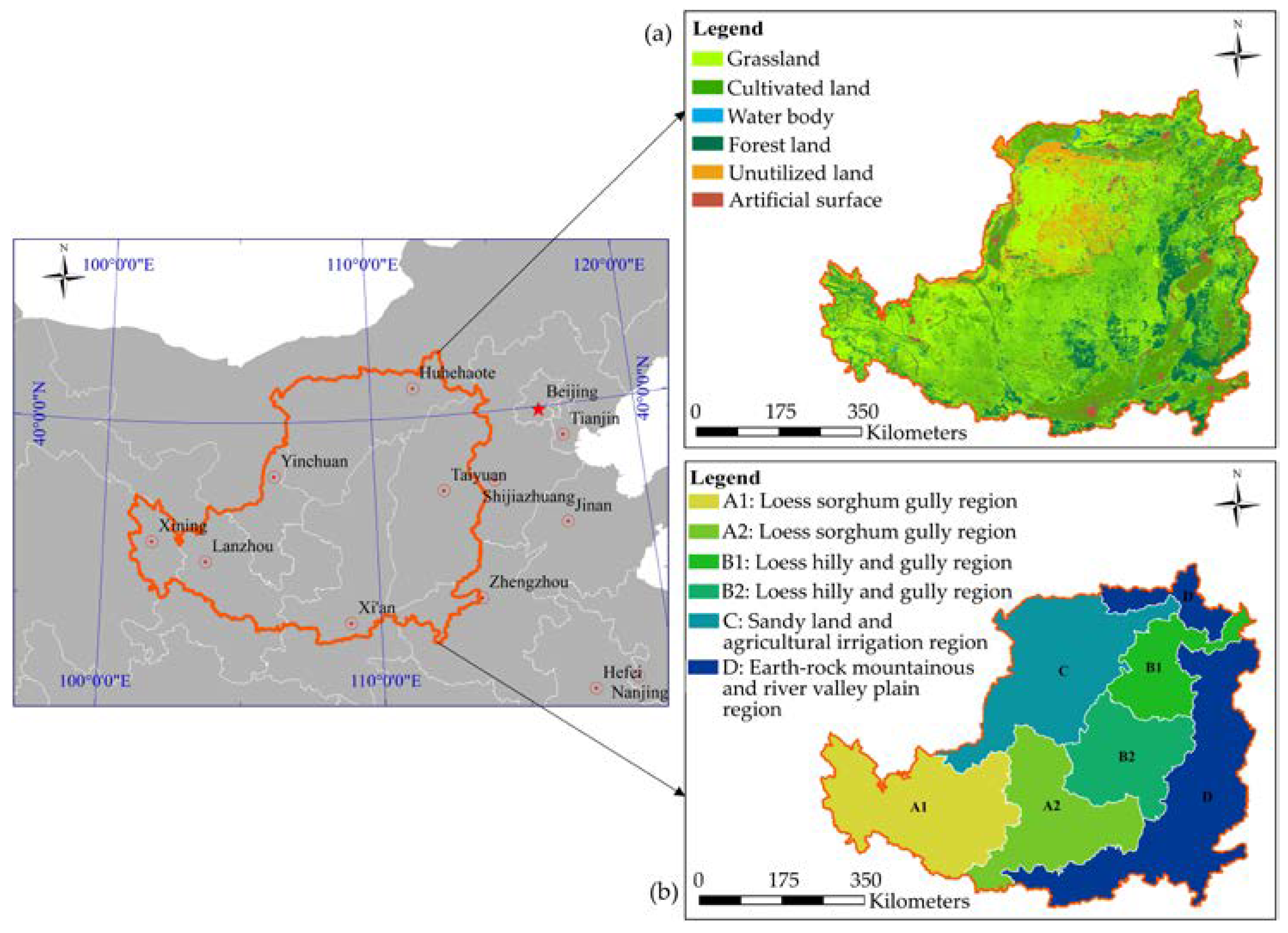
2.1. Study Area
2.2. Data Sources
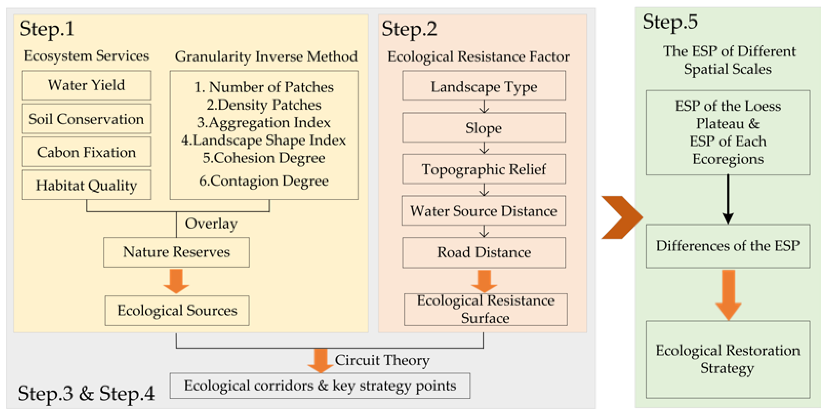
3. Methods
3.1. Determination of Ecological Sources
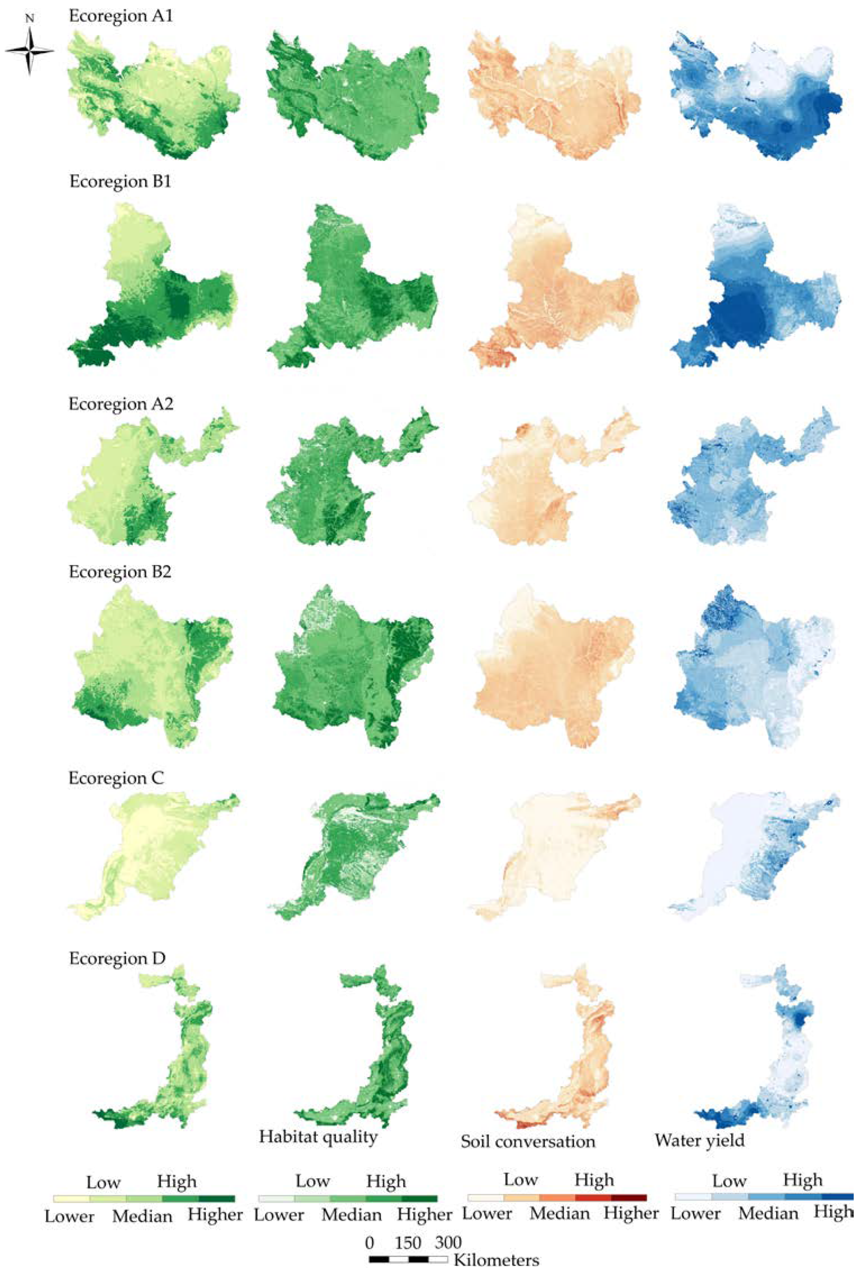
3.1.1. Ecosystem Services
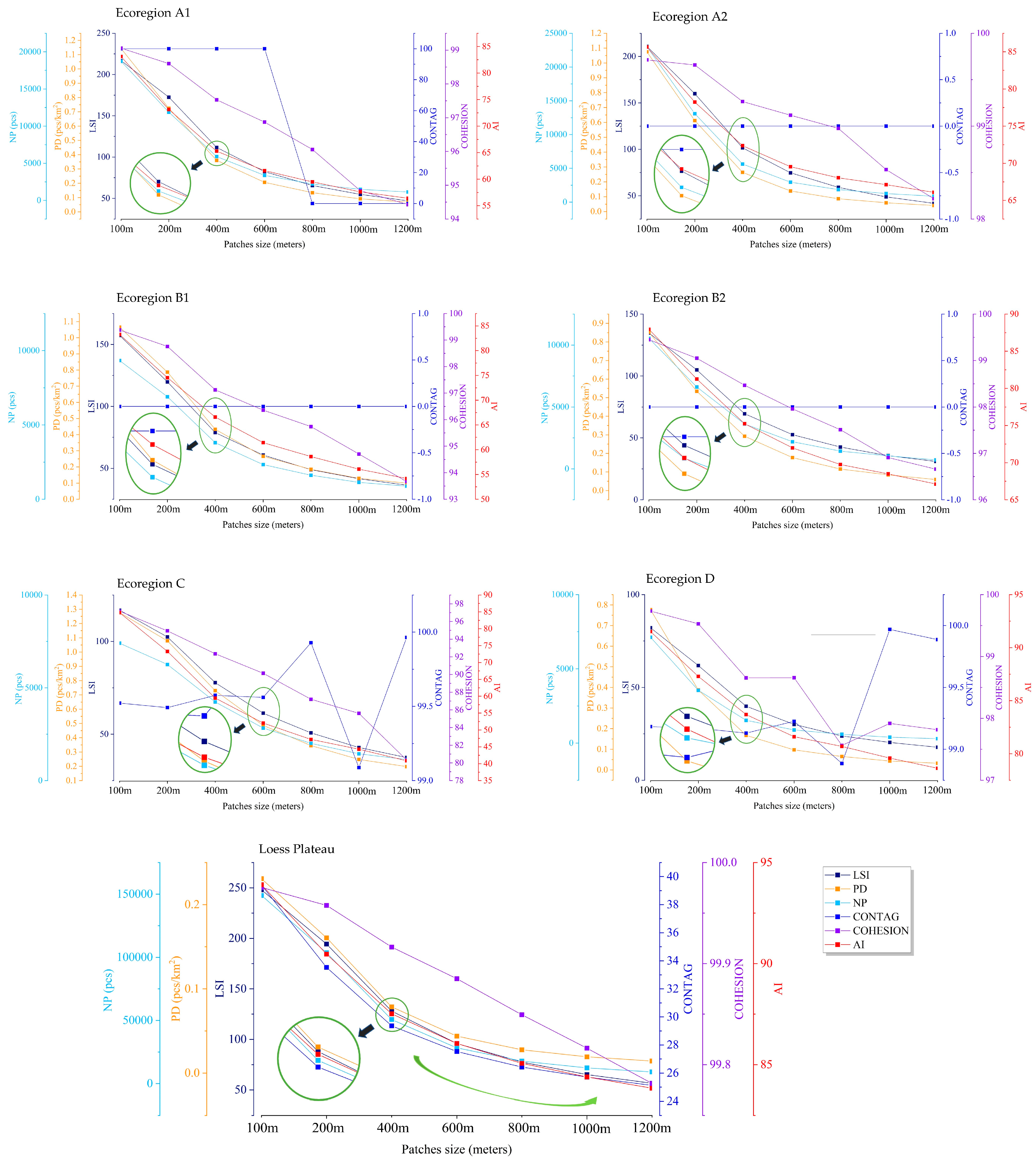
3.1.2. Granularity Inverse Method
3.2. Construction of Ecological Resistance Surface
3.3. Extraction of Ecological Corridor
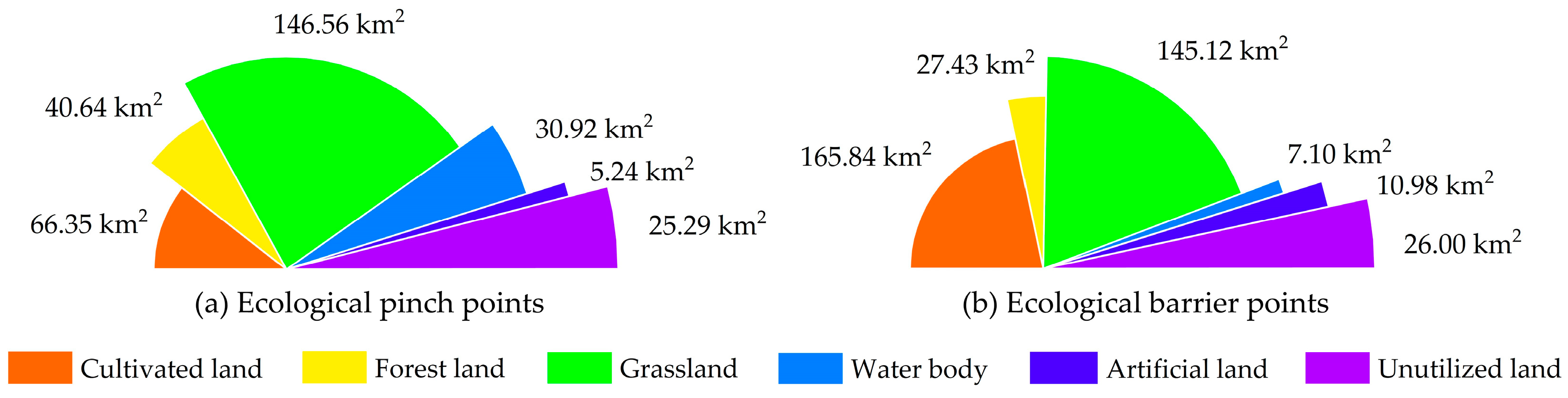
3.4. Identification Ecological Pinch Points and Ecological Barrier Points
4. Results
4.1. Ecological Land Identification
4.2. Ecological Sources
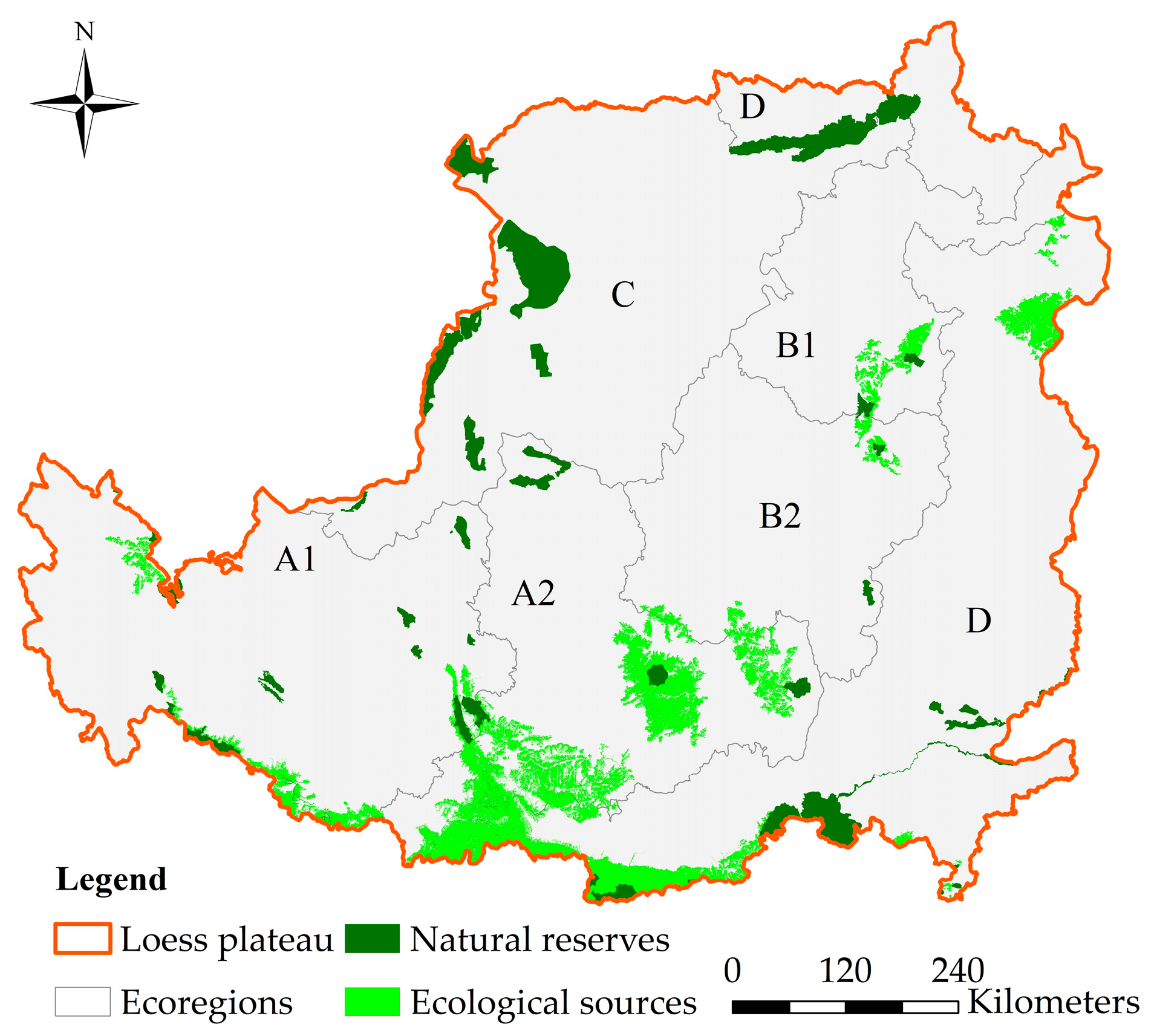
4.2.1. Ecological Sources on the Loess Plateau
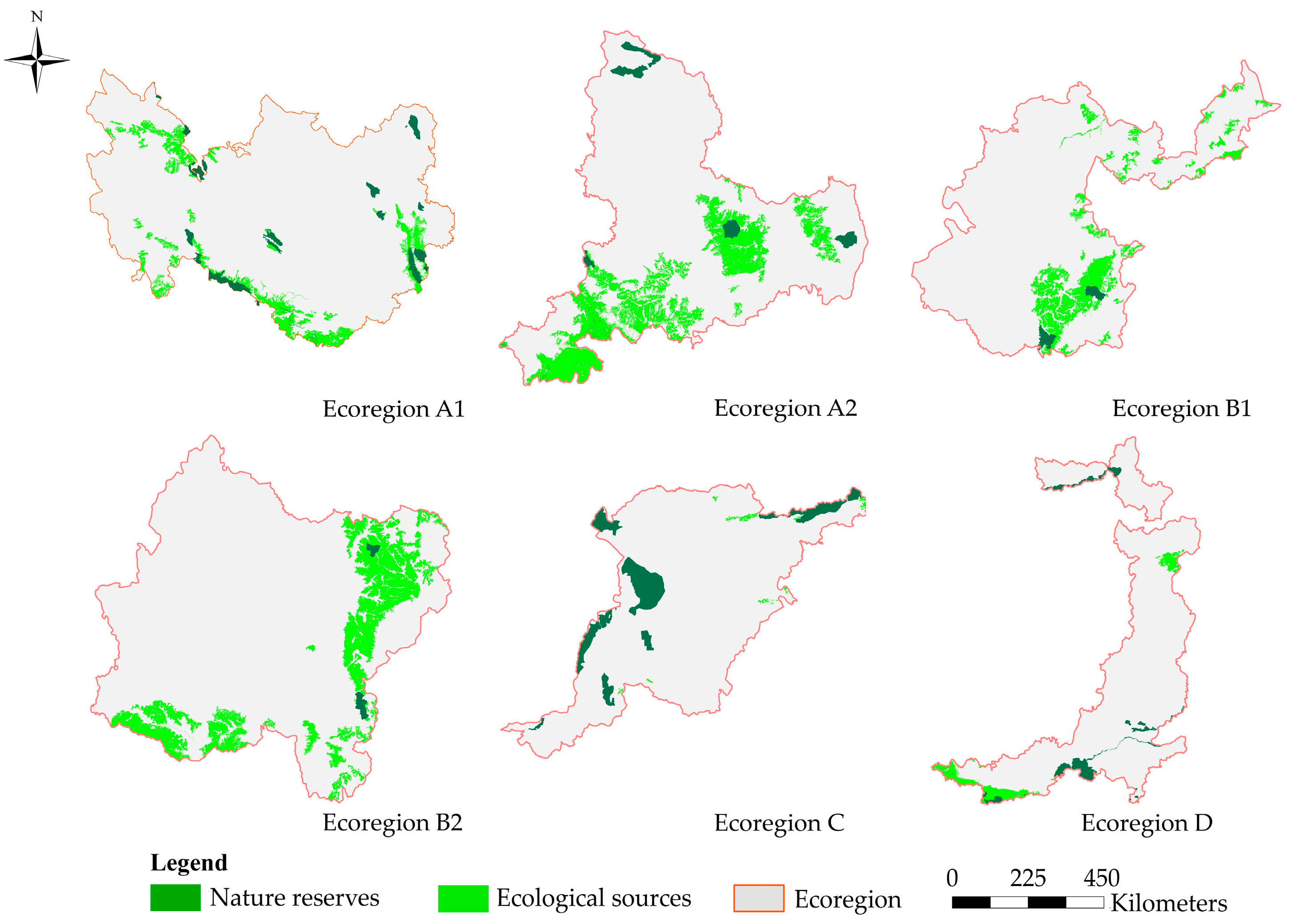
4.2.2. Ecological Sources of Ecoregion
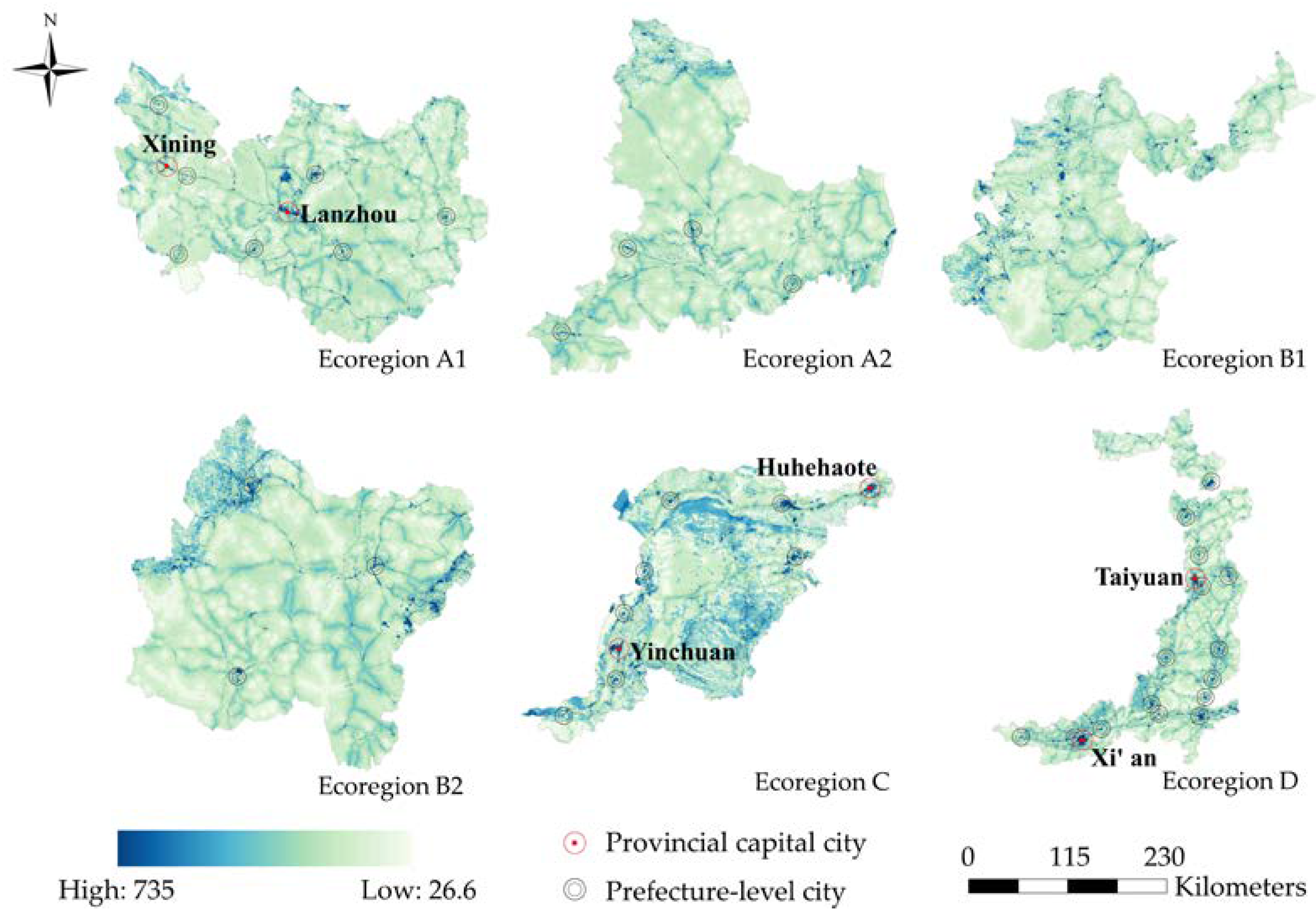
4.3. Ecological Resistance Surface
4.4. Ecological Corridors and Key Strategy Points
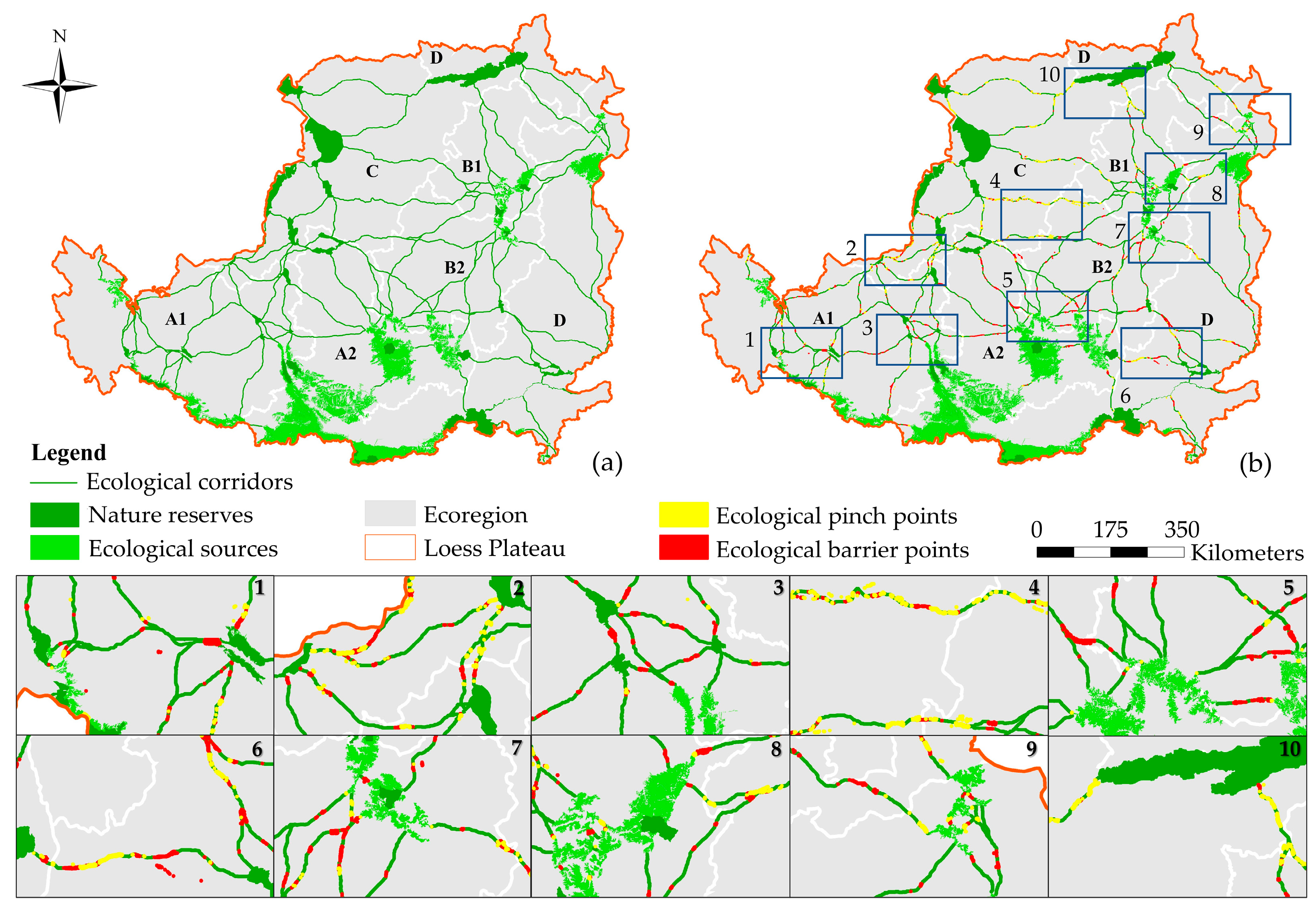
4.4.1. Ecological Corridors and Key Strategy Points of the Loess Plateau
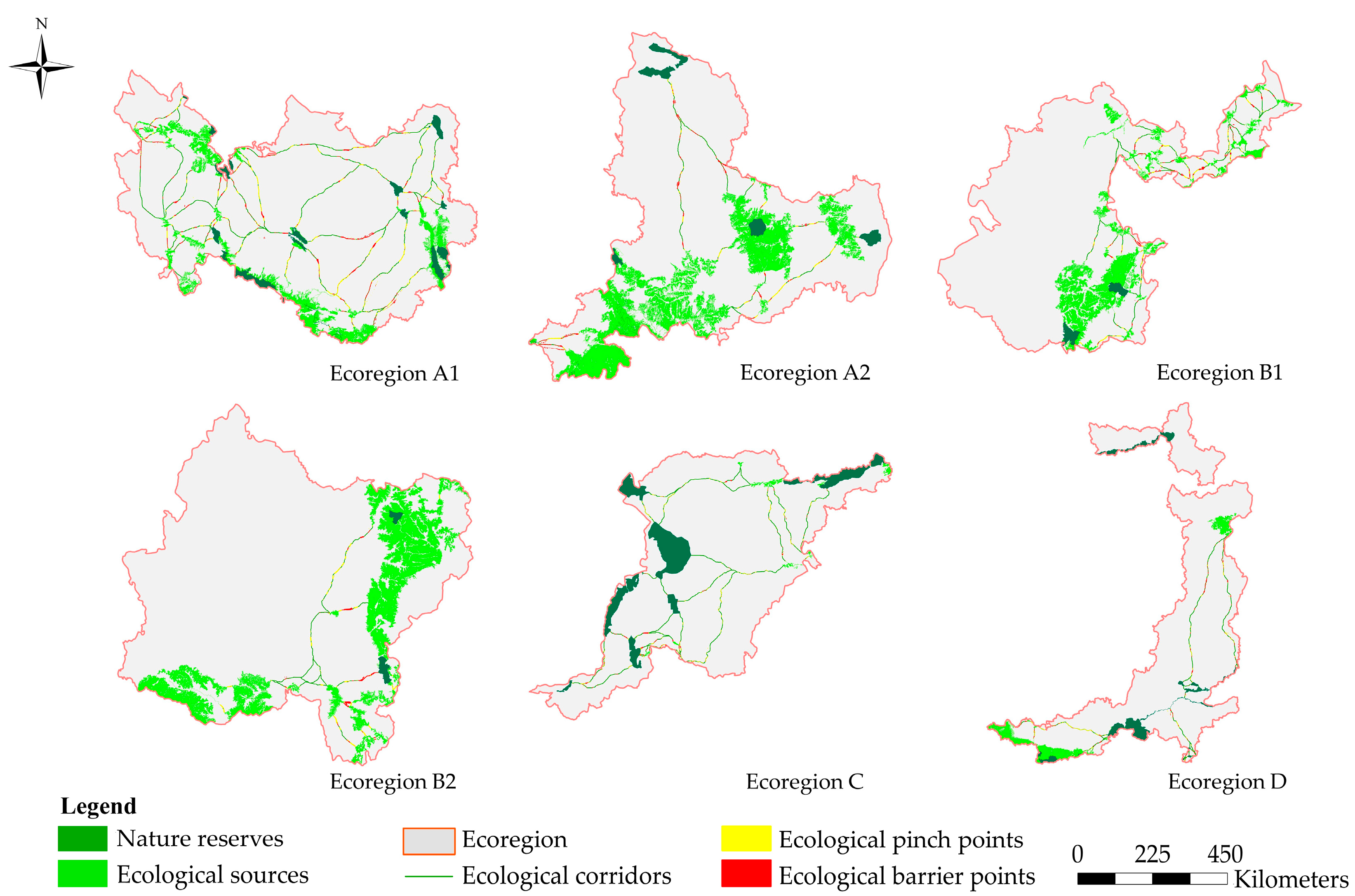
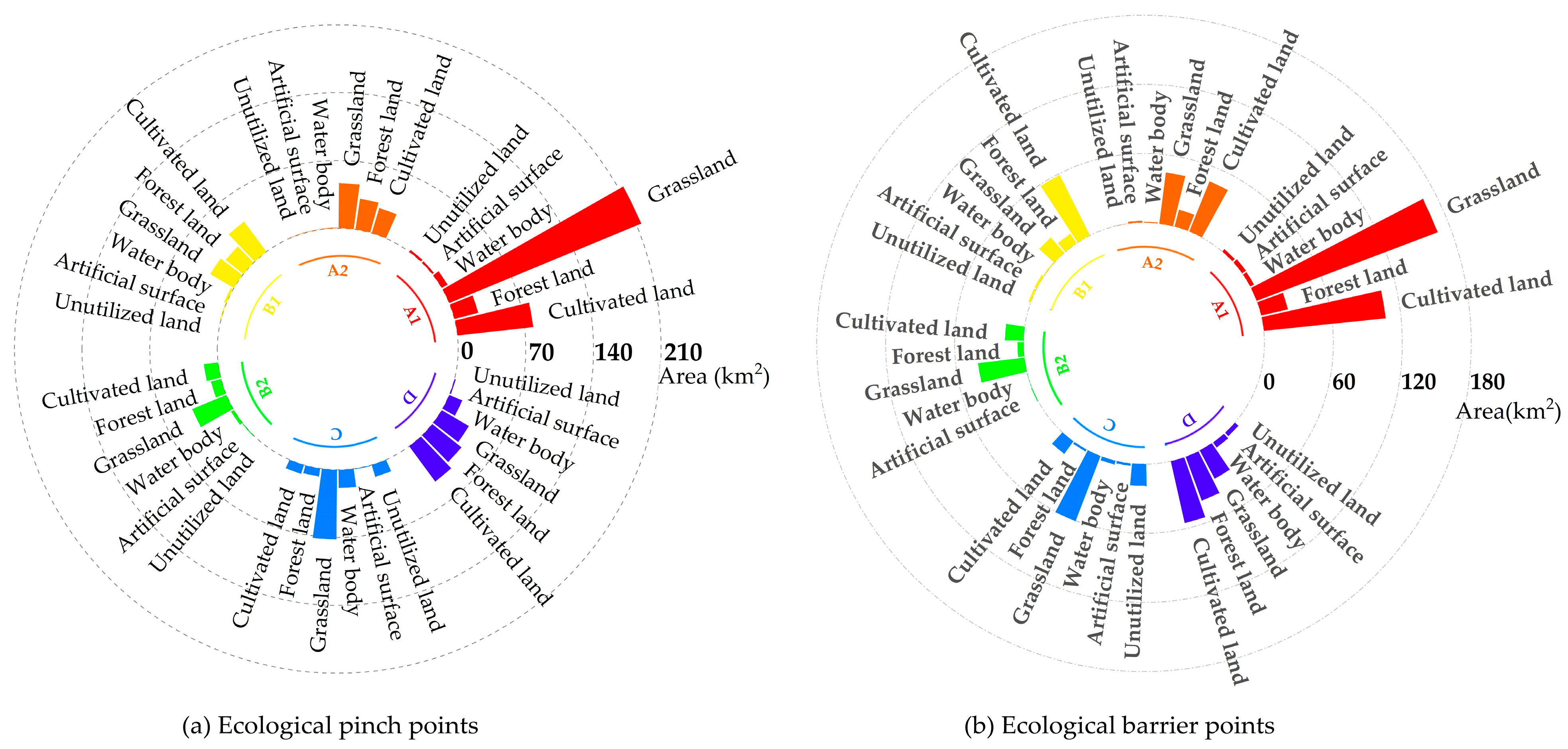
4.4.2. Ecological Corridors and Key Strategy Points of Ecoregions
4.5. ESPs Variation at Different Spatial Scales
5. Discussion
5.1. Optimal Landscape Structure
5.2. Distribution of ESPs and Restoration Strategies
5.3. Comparison of ESPs at Different Spatial Scales
5.4. Significance of ESPs on the Loess Plateau
6. Conclusions
Author Contributions
Funding
Data Availability Statement
Acknowledgments
Conflicts of Interest
References
- Luo, P.P.; Zheng, Y.; Wang, Y.Y.; Zhang, S.P.; Yu, W.Q.; Zhu, X.; Huo, A.D.; Wang, Z.H.; He, B.; Nover, D. Comparative Assessment of Sponge City Constructing in Public Awareness, Xi’an, China. Sustainability 2022, 14, 11653. [Google Scholar] [CrossRef]
- Zhu, W.; Zha, X.; Luo, P.; Wang, S.; Cao, Z.; Lyu, J.; Zhou, M.; He, B.; Nover, D. A quantitative analysis of research trends in flood hazard assessment. Stoch. Environ. Res. Risk Assess. 2023, 37, 413–428. [Google Scholar] [CrossRef]
- Zhu, W.; Wang, S.T.; Luo, P.P.; Zha, X.B.; Cao, Z.; Lyu, J.Q.; Zhou, M.M.; He, B.; Nover, D. A Quantitative Analysis of the Influence of Temperature Change on the Extreme Precipitation. Atmosphere 2022, 13, 612. [Google Scholar] [CrossRef]
- Deng, H.J.; Pepin, N.C.; Chen, Y.N.; Guo, B.; Zhang, S.H.; Zhang, Y.Q.; Chen, X.W.; Gao, L.; Liu, M.B. Dynamics of Diurnal Precipitation Differences and Their Spatial Variations in China. J. Appl. Meteorol. Climatol. 2022, 61, 1015–1027. [Google Scholar] [CrossRef]
- Cao, Z.; Wang, S.T.; Luo, P.P.; Xie, D.N.; Zhu, W. Watershed Ecohydrological Processes in a Changing Environment: Opportunities and Challenges. Water 2022, 14, 1502. [Google Scholar] [CrossRef]
- Duan, W.L.; Zou, S.; Christidis, N.; Schaller, N.; Chen, Y.N.; Sahu, N.; Li, Z.; Fang, G.H.; Zhou, B.T. Changes in temporal inequality of precipitation extremes over China due to anthropogenic forcings. Npj Clim. Atmos. Sci. 2022, 5, 33. [Google Scholar] [CrossRef]
- Serra-Llobet, A.; Hermida, M.A. Opportunities for green infrastructure under Ecuador’s new legal framework. Landsc. Urban Plan. 2017, 159, 1–4. [Google Scholar] [CrossRef]
- Cao, Z.; Zhu, W.; Luo, P.P.; Wang, S.T.; Tang, Z.M.; Zhang, Y.Z.; Guo, B. Spatially Non-Stationary Relationships between Changing Environment and Water Yield Services in Watersheds of China’s Climate Transition Zones. Remote Sens. 2022, 14, 5078. [Google Scholar] [CrossRef]
- Balensiefer, M.; Rossi, R.; Ardinghi, N.; Cenni, M.; Ugolini, M. SER International Primer on Ecological Restoration. Tucson. 2004. Available online: www.ser.org (accessed on 20 January 2023).
- Wang, Z.; Luo, P.P.; Zha, X.B.; Xu, C.Y.; Kang, S.X.; Zhou, M.M.; Nover, D.; Wang, Y.H. Overview assessment of risk evaluation and treatment technologies for heavy metal pollution of water and soil. J. Clean. Prod. 2022, 379, 134043. [Google Scholar] [CrossRef]
- Aronson, J.; Alexander, S. Ecosystem restoration is now a global priority: Time to roll up our sleeves. Restor. Ecol. 2013, 21, 293–296. [Google Scholar] [CrossRef]
- Aronson, J.; Clewell, A.; Moreno-Mateos, D. Ecological restoration and ecological engineering: Complementary or indivisible? Ecol. Eng. 2016, 91, 392–395. [Google Scholar] [CrossRef]
- Peng, J.; Pan, Y.; Liu, Y.; Zhao, H.; Wang, Y. Linking ecological degradation risk to identify ecological security patterns in a rapidly urbanizing landscape. Habitat Int. 2018, 71, 110–124. [Google Scholar] [CrossRef]
- Zha, X.B.; Luo, P.P.; Zhu, W.; Wang, S.T.; Lyu, J.Q.; Zhou, M.M.; Huo, A.D.; Wang, Z.H. A Bibliometric Analysis of the Research on Sponge City: Current Situation and Future Development Direction. Ecohydrology 2021, 14, e2328. [Google Scholar] [CrossRef]
- Bai, H.; Li, Z.W.; Guo, H.L.; Chen, H.P.; Luo, P.P. Urban Green Space Planning Based on Remote Sensing and Geographic Information Systems. Remote Sens. 2022, 14, 4213. [Google Scholar] [CrossRef]
- Peng, J.; Yang, Y.; Liu, Y.; Du, Y.; Meersmans, J.; Qiu, S. Linking ecosystem services and circuit theory to identify ecological security patterns. Sci. Total Environ. 2018, 644, 781–790. [Google Scholar] [CrossRef]
- Ni, Q.L.; Hou, H.P.; Ding, Z.Y.; Li, Y.B.; Li, J.R. Ecological remediation zoning of territory based on the ecological security pattern recognition: Taking Jiawang district of Xuzhou city as an example. J. Nat. Resour. 2020, 35, 204–216. [Google Scholar] [CrossRef]
- Luo, P.P.; Xu, C.; Kang, S.; Huo, A.; Lyu, J.; Zhou, M.; Nover, D. Heavy metals in water and surface sediments of the Fenghe River Basin, China: Assessment and source analysis. Water Sci. Technol. 2021, 84, 3072–3090. [Google Scholar] [CrossRef]
- Chen, X.; Peng, J.; Liu, Y.X.; Yang, Y.; Li, G.C. Constructing ecological security patterns in Yunfu city based on the framework of importance-sensitivity-connectivity. Geogr. Res. 2017, 36, 471–484. [Google Scholar] [CrossRef]
- Huang, L.Y.; Liu, S.H.; Fang, Y.; Zou, L. Construction of Wuhan’s ecological security pattern under the “quality-risk-requirement” framework. J. Appl. Ecol. 2019, 30, 615–626. [Google Scholar] [CrossRef]
- Kukkala, A.S.; Moilanen, A. Ecosystem services and connectivity in spatial conservation prioritization. Landsc. Ecol. 2017, 32, 5–14. [Google Scholar] [CrossRef]
- Luo, P.P.; Luo, M.T.; Li, F.Y.; Qi, X.G.; Huo, A.D.; Wang, Z.H.; He, B.; Takara, K.; Nover, D.; Wang, Y. Urban flood numerical simulation: Research, methods and future perspectives. Environ. Model. Softw. 2022, 156, 105478. [Google Scholar] [CrossRef]
- Duan, W.L.; Zou, S.; Chen, Y.N.; Nover, D.; Fang, G.H.; Wang, Y. Sustainable water management for cross-border resources: The Balkhash Lake Basin of Central Asia, 1931–2015. J. Clean. Prod. 2020, 263, 121614. [Google Scholar] [CrossRef]
- Hu, Y.N.; Duan, W.L.; Chen, Y.N.; Zou, S.; Kayumba, P.M.; Qin, J.X. Exploring the changes and driving forces of water footprint in Central Asia: A global trade assessment. J. Clean. Prod. 2022, 375, 134062. [Google Scholar] [CrossRef]
- Wang, D.; Chen, J.; Zhang, L.; Sun, Z.; Wang, X.; Zhang, X.; Zhang, W. Establishing an ecological security pattern for urban agglomeration, taking ecosystem services and human interference factors into consideration. PeerJ 2019, 7, e7306. [Google Scholar] [CrossRef]
- Wei, S.M.; Pan, J.H.; Liu, X. Landscape ecological safety assessment and landscape pattern optimization in arid inland river basin: Take Ganzhou District as an example. Hum. Ecol. Risk Assess. Int. J. 2020, 26, 782–806. [Google Scholar] [CrossRef]
- Gurrutxaga, M.; Rubio, L.; Saura, S. Key connectors in protected forest area networks and the impact of highways: A transnational case study from the Cantabrian Range to the Western Alps (SW Europe). Landsc. Urban Plan. 2011, 101, 310–320. [Google Scholar] [CrossRef]
- Kong, F.; Yin, H.; Nakagoshi, N.; Zong, Y. Urban green space network development for biodiversity conservation: Identification based on graph theory and gravity modeling. Landsc. Urban Plan. 2010, 95, 16–27. [Google Scholar] [CrossRef]
- Han, Z.W.; Jiao, S.; Hu, L.; Yang, Y.M.; Cai, Q.; Li, B.; Zhou, M. Construction of ecological security pattern based on coordination between corridors and sources in national territorial space. J. Nat. Resour. 2019, 34, 2244–2256. [Google Scholar] [CrossRef]
- Xiao, S.H.; Wu, W.J.; Guo, J.; Ou, M.H.; Pueppke, S.G.; Ou, W.X.; Tao, Y. An evaluation framework for designing ecological security patterns and prioritizing ecological corridors: Application in Jiangsu Province, China. Landsc. Ecol. 2020, 35, 2517–2534. [Google Scholar] [CrossRef]
- Carroll, C.; Roberts, D.R.; Michalak, J.L.; Lawler, J.J.; Nielsen, S.E.; Stralberg, D.; Hamann, A.; Mcrae, B.H.; Wang, T.L. Scale-dependent complementarity of climatic velocity and environmental diversity for identifying priority areas for conservation under climate change. Glob. Chang. Biol. 2017, 23, 4508–4520. [Google Scholar] [CrossRef]
- Wang, S.T.; Luo, P.P.; Xu, C.Y.; Zhu, W.; Cao, Z.; Ly, S. Reconstruction of Historical Land Use and Urban Flood Simulation in Xi’an, Shannxi, China. Remote Sens. 2022, 14, 6067. [Google Scholar] [CrossRef]
- Proctor, M.F.; Nielsen, S.E.; Kasworm, W.F.; Servheen, C.; Radandt, T.G.; Machutchon, A.G.; Boyce, M.S. Grizzly bear connectivity mapping in the Canada–United States trans-border region. J. Wildl. Manag. 2015, 79, 544–558. [Google Scholar] [CrossRef]
- McRae, B.H.; Dickson, B.G.; Keitt, T.H.; Shah, V.B. Using circuit theory to model connectivity in ecology, evolution, and conservation. Ecology 2008, 89, 2712–2724. [Google Scholar] [CrossRef] [PubMed]
- Jing, P.Q.; Zhang, D.H.; Ai, Z.M.; Guo, B. Natural landscape ecological risk assessment based on the three-dimensional framework of pattern-process ecological adaptability cycle: A case in Loess Plateau. Acta Ecol. Sin. 2021, 41, 7026–7036. [Google Scholar] [CrossRef]
- Zhu, Y.H.; Luo, P.P.; Zhang, S.; Sun, B. Spatiotemporal Analysis of Hydrological Variations and Their Impacts on Vegetation in Semiarid Areas from Multiple Satellite Data. Remote Sens. 2020, 12, 4177. [Google Scholar] [CrossRef]
- Jin, F.; Yang, W.; Fu, J.; Li, Z. Effects of vegetation and climate on the changes of soil erosion in the Loess Plateau of China. Sci. Total Environ. 2021, 773, 145514. [Google Scholar] [CrossRef]
- Hou, H.P.; Ding, Z.Y.; Zhang, S.L.; Guo, S.C.; Yang, Y.J.; Chen, Z.X.; Mi, J.X.; Wang, X. Spatial estimate of ecological and environmental damage in an underground coal mining area on the Loess Plateau: Implications for planning restoration interventions. J. Clean. Prod. 2021, 287, 125061. [Google Scholar] [CrossRef]
- Luo, P.P.; Liu, L.M.; Wang, S.T.; Ren, B.M.; He, B.; Nover, D. Influence assessment of new Inner Tube Porous Brick with absorbent concrete on urban floods control. Case Stud. Constr. Mater. 2022, 17, e01236. [Google Scholar] [CrossRef]
- Feng, Q.; Zhao, W.; Hu, X.; Liu, Y.; Daryanto, S.; Cherubini, F. Trading-off ecosystem services for better ecological restoration: A case study in the Loess Plateau of China. J. Clean. Prod. 2020, 257, 120469. [Google Scholar] [CrossRef]
- Wu, X.; Wang, S.; Fu, B.; Liu, J. Spatial variation and influencing factors of the effectiveness of afforestation in China’s Loess Plateau. Sci. Total Environ. 2021, 771, 144904. [Google Scholar] [CrossRef] [PubMed]
- Pan, J.H.; Li, L. Optimization of ecological security pattern in Gansu section of the Yellow River Basin using OWA and circuit model. Trans. Chin. Soc. Agric. Eng. 2021, 37, 259–268. [Google Scholar] [CrossRef]
- He, J.; Shi, X.Y.; Fu, Y.J. Optimization of ecological security pattern in the source area of Fenhe River Basin based on ecosystem services. J. Nat. Resour. 2020, 35, 814–825. [Google Scholar] [CrossRef]
- Peng, J.; Zhao, H.J.; Liu, Y.X.; Wu, J.S. Research progress and prospect on regional ecological security pattern construction. Geogr. Res. 2017, 36, 407–419. [Google Scholar] [CrossRef]
- Jing, Y.C.; Chen, L.D.; Sun, R.H. A theoretical research framework for ecological security pattern construction based on ecosystem services supply and demand. Acta Ecol. Sin. 2018, 38, 4121–4131. [Google Scholar] [CrossRef]
- Altman, I.; Blakeslee, A.M.; Osio, G.C.; Rillahan, C.B.; Teck, S.J.; Meyer, J.J.; Byers, J.E.; Rosenberg, A.A. A practical approach to implementation of ecosystem-based management: A case study using the Gulf of Maine marine ecosystem. Front. Ecol. Environ. 2011, 9, 183–189. [Google Scholar] [CrossRef]
- Heenan, A.; Gorospe, K.; Williams, I.; Levine, A.; Maurin, P.; Nadon, M.; Oliver, T.; Rooney, J.; Timmers, M.; Wongbusarakum, S.; et al. Ecosystem monitoring for ecosystem-based management: Using a polycentric approach to balance information trade-offs. J. Appl. Ecol. 2016, 53, 699–704. [Google Scholar] [CrossRef]
- Yang, Y.; Wang, B.; Wang, G.; Li, Z. Ecological regionalization and overview of the Loess Plateau. Acta Ecol. Sin. 2019, 39, 7389–7397. [Google Scholar] [CrossRef]
- Yuan, Y.; Bai, Z.K.; Shi, X.Y.; Zhao, X.Q.; Zhang, J.N.; Yang, B.Y. Determining priority areas for ecosystem preservation and restoration of territory based on ecological security pattern: A case study in Zunhua City, Hebei Province. Chin. J. Ecol. 2022, 41, 750–759. [Google Scholar] [CrossRef]
- Wei, X.D.; Lin, L.G.; Feng, X.L.; Wang, X.F.; Kong, D.H.; Lin, K.L.; Yang, J. Construction of ecological security pattern and quantitative diagnosis of ecological problems in Shenmu City. Acta Ecol. Sin. 2023, 43, 1–13. [Google Scholar] [CrossRef]
- Van Oost, K.; Govers, G.; Desmet, P. Evaluating the effects of changes in landscape structure on soil erosion by water and tillage. Landsc. Ecol. 2000, 15, 577–589. [Google Scholar] [CrossRef]
- Duan, W.L.; Maskey, S.; Chaffe, P.L.B.; Luo, P.P.; He, B.; Wu, Y.P.; Hou, J.M. Recent advancement in remote sensing technology for hydrology analysis and water resources management. Remote Sens. 2021, 13, 1097. [Google Scholar] [CrossRef]
- Zhang, J.; Liu, M.; Zhang, M.; Yang, J.; Cao, R.; Malhi, S.S. Changes of vegetation carbon sequestration in the tableland of Loess Plateau and its influencing factors. Environ. Sci. Pollut. Res. 2019, 26, 22160–22172. [Google Scholar] [CrossRef]
- Li, Y.; Zhang, P.; Qin, Y. Ecological service evaluation: An empirical study on the Central Loess Plateau, China. Pol. J. Environ. Stud. 2020, 29, 1691–1701. [Google Scholar] [CrossRef]
- Zhu, C.; Zhang, X.; Zhou, M.; He, S.; Gan, M.; Yang, L.; Wang, K. Impacts of urbanization and landscape pattern on habitat quality using OLS and GWR models in Hangzhou, China. Ecol. Indic. 2020, 117, 106654. [Google Scholar] [CrossRef]
- Guan, D.; Jiang, Y.; Cheng, L. How can the landscape ecological security pattern be quantitatively optimized and effectively evaluated? An integrated analysis with the granularity inverse method and landscape indicators. Environ. Sci. Pollut. Res. 2022, 29, 41590–41616. [Google Scholar] [CrossRef]
- Lu, Y.; She, J.Y.; Chen, C.H.; She, Y.C.; Luo, G.G. Landscape ecological security pattern optimization based on the granularity inverse method: A case study in Xiuying district, Haikou. Acta Ecol. Sin. 2015, 35, 6384–6393. [Google Scholar] [CrossRef]
- Xiao, L.; Cui, L.; Jiang, Q.O.; Wang, M.; Xu, L.; Yan, H. Spatial structure of a potential ecological network in Nanping, China, based on ecosystem service functions. Land 2020, 9, 376. [Google Scholar] [CrossRef]
- Beier, P.; Majka, D.R.; Spencer, W.D. Forks in the road: Choices in procedures for designing wildland linkages. Conserv. Biol. 2008, 22, 836–851. [Google Scholar] [CrossRef]
- Spear, S.F.; Balkenhol, N.; Fortin, M.J.; McRae, B.H.; Scribner, K. Use of resistance surfaces for landscape genetic studies: Considerations for parameterization and analysis. Mol. Ecol. 2010, 19, 3576–3591. [Google Scholar] [CrossRef]
- Liu, J.L.; Li, S.P.; Fan, S.L.; Hu, Y. Identification of territorial ecological protection and restoration areas and early warning places based on ecological security pattern: A case study in Xiamen-Zhangzhou-Quanzhou Region. Acta Ecol. Sin. 2021, 41, 8124–8134. [Google Scholar] [CrossRef]
- Fang, Y.; Wang, J.; Huang, L.Y.; Zhai, T.L. Determining and identifying key areas of ecosystem preservation and restoration for territorial spatial planning based on ecological security patterns: A case study of Yantai city. J. Nat. Resour. 2020, 35, 01000190. [Google Scholar] [CrossRef]
- Carroll, C.; McRAE, B.H.; Brookes, A. Use of linkage mapping and centrality analysis across habitat gradients to conserve connectivity of gray wolf populations in western North America. Conserv. Biol. 2012, 26, 78–87. [Google Scholar] [CrossRef] [PubMed]
- McRae, B.H.; Hall, S.A.; Beier, P.; Theobald, D.M. Where to restore ecological connectivity? Detecting barriers and quantifying restoration benefits. PLoS ONE 2012, 7, e52604. [Google Scholar] [CrossRef]
- Yu, H.; Gu, X.; Liu, G.; Fan, X.; Zhao, Q.; Zhang, Q. Construction of Regional Ecological Security Patterns Based on Multi-Criteria Decision Making and Circuit Theory. Remote Sens. 2022, 14, 527. [Google Scholar] [CrossRef]
- Zhang, J.; Qu, M.; Wang, C.; Zhao, J.; Cao, Y. Quantifying landscape pattern and ecosystem service value changes: A case study at the county level in the Chinese Loess Plateau. Glob. Ecol. Conserv. 2020, 23, e01110. [Google Scholar] [CrossRef]
- Li, G.; Fang, C.; Wang, S. Exploring spatiotemporal changes in ecosystem-service values and hotspots in China. Sci. Total Environ. 2016, 545, 609–620. [Google Scholar] [CrossRef]
- Zhao, X.Y.; Ma, P.Y.; Li, W.Q.; Du, Y.X. Spatiotemporal changes of supply and demand relationships of ecosystem services in the Loess Plateau. Acta Geogr. Sin. 2021, 76, 2780–2796. [Google Scholar] [CrossRef]
- Tang, L.; Luo, Y.Y.; Luo, G.G.; Li, J.; Liu, Q.C.; Li, J.Z. Landscape pattern optimization based on the granularity inverse method and MCR model in Dongfang City, Hainan Province. Chin. J. Ecol. 2016, 35, 3393–3403. [Google Scholar] [CrossRef]
- Chen, C.; Shi, L.; Lu, Y.; Yang, S.; Liu, S. The optimization of urban ecological network planning based on the minimum cumulative resistance model and granularity reverse method: A case study of Haikou, China. IEEE Access 2020, 8, 43592–43605. [Google Scholar] [CrossRef]
- Wang, S.T.; Cao, Z.; Luo, P.P.; Zhu, W. Spatiotemporal Variations and Climatological Trends in Precipitation Indices in Shaanxi Province, China. Atmosphere 2022, 13, 744. [Google Scholar] [CrossRef]
- Chen, Q.Q. Research on Territorial Space Ecological Restoration Strategies Based on Ecological Security Patterns—A Case Study of Binzhou City. Master’s Degree, Zhejiang University, Hangzhou, China, 14 May 2021. [Google Scholar]
- Luo, P.P.; Mu, Y.; Wang, S.T.; Zhu, W.; Mishra, B.K.; Huo, A.D.; Zhou, M.M.; Lyu, L.Q.; Hu, M.C.; Duan, W.L.; et al. Exploring sustainable solutions for the water environment in Chinese and Southeast Asian cities. Ambio 2021, 51, 1199–1218. [Google Scholar] [CrossRef]
- Li, C.; Li, J. Assessing urban sustainability using a multi-scale, theme-based indicator framework: A case study of the Yangtze River Delta region, China. Sustainability 2017, 9, 2072. [Google Scholar] [CrossRef]
- Qin, J.X.; Duan, W.L.; Chen, Y.N.; Dukhovny, V.A.; Sorokin, D.; Li, Y.P.; Wang, X.X. Comprehensive evaluation and sustainable development of water–energy–food–ecology systems in Central Asia. Renew. Sustain. Energy Rev. 2022, 157, 112061. [Google Scholar] [CrossRef]
- Zhao, L. Landscape Ecological Risk Assessment and Ecological Security Pattern Construction in Mining City: A Case Study of Wu’an City; China University of Geosciences: Beijing, China, 2020. [Google Scholar] [CrossRef]
- Tian, Y.; Feng, Q.; Tang, M.; Zheng, S.; Liu, C.; Wu, D.; Wang, L. Ecological protection and restoration of forest, wetland, grassland and cropland based on the perspective of ecosystem assessment: A case study in wuliangsuhai watershed. Acta Ecol. Sin. 2019, 39, 8826–8836. [Google Scholar] [CrossRef]
- Fu, B.J. Several key points in territorial ecological restoration. Bull. Chin. Acad. Sci. Chin. Version 2021, 36, 64–69. [Google Scholar] [CrossRef]
- Song, W.; Han, Z.; Liu, L. Systematic diagnosis of ecological problems and comprehensive zoning of ecological conservation and restoration for an integrated ecosystem of mountains-rivers-forests-farmlands-lakes-grasslands in Shaanxi Province. Acta Ecol. Sin. 2019, 39, 8975–8989. [Google Scholar] [CrossRef]
- Jiang, W.; Fu, B.; Lü, Y. Assessing impacts of land use/land cover conversion on changes in ecosystem services value on the Loess Plateau, China. Sustainability 2020, 12, 7128. [Google Scholar] [CrossRef]
- Jiang, C.; Yang, Z.Y.; Wen, M.L.; Huang, L.; Liu, H.M.; Wang, J.; Chen, W.L.; Zhuang, C.W. Identifying the spatial disparities and determinants of ecosystem service balance and their implications on land use optimization. Sci. Total Environ. 2021, 793, 148472. [Google Scholar] [CrossRef]
- Zhou, W.; Guan, Y.J.; Liu, Q.; Fan, Y.B.; Bai, Z.K.; Shi, X.Y.; Hu, Y.C.; Huang, Y.H.; Bai, D.S. Diagnosis of ecological problems and exploration of ecosystem restoration practices in the typical watershed of loess plateau: A case study of the pilot project in the middle and upper reaches of Fen River in Shanxi Province. Acta Ecol. Sin. 2019, 39, 8817–8825. [Google Scholar] [CrossRef]
- United Nations. Transforming Our World: The 2030 Agenda for Sustainable Development; United Nations: New York, NY, USA, 2015. [Google Scholar]
- Fan, X.; Rong, Y.J.; Tian, C.X.; Ou, S.Y.; Li, J.F.; Shi, H.; Qin, Y.; He, J.W.; Huang, C.B. Construction of an Ecological Security Pattern in an Urban–Lake Symbiosis Area: A Case Study of Hefei Metropolitan Area. Remote Sens. 2022, 14, 2498. [Google Scholar] [CrossRef]


| Ecoregion | Areas/km2 | Characteristic |
|---|---|---|
| A1 and A2: Loess sorghum gully region | 217,851.98 km2 | The surface of the loess tableland is flat and broad, but is surrounded by deep gully loess highlands. The region has high annual precipitation and abundant heat and light resources, but soil erosion is relatively serious. |
| B1 and B2: Loess hilly and gully region | 125,499.25 km2 | The landscape is dominated by mount and beam-like hills, with long gullies and broken terrain. The climate is arid and soil erosion is serious. |
| C: Sandy land and agricultural irrigation region | 130,060.30 km2 | The sandy land is dominated by the Mao Wu Su sandy land, with an arid climate and small water erosion modulus. The agricultural irrigation area has flat terrain and is dominated by irrigation water sources. Soil erosion is relatively low. |
| D: Earth-rock mountainous and river valley plain region | 175,883.58 km2 | Mountainous area is mostly covered by thin layers of loess with good vegetation conditions, forming an important water conservation area. The river valley plains are low and flat with sufficient water, low soil erosion, and abundant light and heat resources. |
| Data | Format | Data Description |
|---|---|---|
| Land use | Raster | Used to assess habitat quality, a parameter of water yield and soil conservation |
| NDVI | Raster | Used to calculate Fraction Vegetation Coverage (FVC), a parameter of the crop management factor |
| NPP | Raster | Used to calculate carbon fixation |
| DEM | Raster | Used to calculate sub-basins, slope lengths, slopes, and topographic relief |
| LAI | Raster | Used to calculate annual average evapotranspiration |
| Temperature and rainfall | Raster | Obtained by interpolation and used to calculate annual average evapotranspiration, to calculate rainfall erosivity factors, and to estimate soil microbial respiration |
| Soil organic matter content, soil texture, soil depth, and root depth | Raster | Used to calculate the root restricting layer depth and the plant available water content (PAWC). |
| Soil erodibility | Raster | One of the parameters of soil conservation calculation |
| River network and road network | Vector | Used to construct the comprehensive resistance surface |
| Nature reserve | Vector | One of the ecological sources |
| Ecosystem Services | Calculation Method | Parameters |
|---|---|---|
| Water yield | Water yield is estimated by the water yield module of the InVEST model (https://www.naturalcapitalproject.org/invest/, accessed on 15 March 2022) [51,52]. In this formula, is the amount of water yield (mm) of pixel of land cover type ; is the annual precipitation of pixel ; is the annual average evapotranspiration (mm) of pixel of land cover type . | |
| Carbon fixation | Carbon fixation is mainly measured using the vegetation net ecosystem productivity (NEP) estimation model [53]. In this formula, where is the vegetation net ecosystem productivity of pixel in year (gC/m2); is the vegetation net primary productivity of pixel in year (gC/m2); is the soil microbial respiration of pixel n in t year (gC/m2). When NEP > 0, it indicates that the carbon fixed by vegetation is greater than that emitted by soil respiration, and vegetation shows the role of carbon sink; when NEP < 0, it indicates that vegetation shows the role of carbon source. | |
| Soil conservation | The amount of soil conservation is calculated using the Revised Universal Soil Loss Equation (RUSLE) [54]. In this formula, A is the amount of soil conservation (t/(hm2·a)); is the rainfall erosivity factor ((MJ·mm)/(hm2·h·a)); is the soil erodibility factor ((t·hm2·h)/(hm2·MJ·mm)); is the terrain factor; is the crop management factor; and is the erosion control practice factor. L, S, C, and P factors are dimensionless. | |
| Habitat quality | Habitat quality is assessed using the habitat quality module of the InVEST model (https://www.naturalcapitalproject.org/invest/, accessed on 15 March 2022) [55]. In this formula, is the habitat quality index of pixel of habitat type ; is the habitat suitability of habitat type ; is the half-saturation constant, which is taken as 0.5 according to the references because it is helpful to intuitively represent the heterogeneity of the whole landscape quality; is the habitat degradation degree of pixel of habitat type ; is the normalization constant, which is usually set to 2.5. |
| Index | Unit | Description |
|---|---|---|
| Number of Patches (NP) | - | Number of landscape patches |
| Density Patches (PD) | - | Density patches in the landscape can reflect the fragmentation degree of a certain landscape type |
| Aggregation Index (AI) | % | Connectivity between patches of each landscape type |
| Landscape Shape Index (LSI) | - | Non-integer dimension of irregular geometry landscape, reflecting the complexity of landscape shape |
| Cohesion Degree (COHESION) | % | Aggregation and dispersion of patches in the landscape |
| Contagion Degree (CONTAG) | % | Agglomeration degree or tendency of patches to spread in a certain landscape |
| Ecological Resistance Factor | Weight | Index | Resistance Coefficient |
|---|---|---|---|
| Landscape type | 0.40 | Woodland | 1 |
| Shrubland | 10 | ||
| Open woodland and other woodlands | 30 | ||
| High coverage grassland | 30 | ||
| Medium coverage grassland | 50 | ||
| Low coverage grassland | 80 | ||
| Water body | 100 | ||
| Water field | 100 | ||
| Dry land | 200 | ||
| Unutilized land | 700 | ||
| Rural residential area | 900 | ||
| Urban land and other construction land | 1000 | ||
| Slope | 0.10 | <8° | 1 |
| 8~15° | 10 | ||
| 15~25° | 50 | ||
| 25~35° | 70 | ||
| >35° | 100 | ||
| Topographic relief | 0.10 | <25 m | 1 |
| 25~50 m | 10 | ||
| 50~70 m | 50 | ||
| 70~100 m | 75 | ||
| >100 m | 100 | ||
| Water source distance | 0.20 | <1000 m | 150 |
| 1000~3000 m | 200 | ||
| 3000~5000 m | 400 | ||
| 5000~10,000 m | 600 | ||
| >10,000 m | 800 | ||
| Road distance | 0.20 | >8000 m | 30 |
| 5000~8000 m | 100 | ||
| 3000~5000 m | 300 | ||
| 1000~3000 m | 500 | ||
| <1000 m | 800 |
Disclaimer/Publisher’s Note: The statements, opinions and data contained in all publications are solely those of the individual author(s) and contributor(s) and not of MDPI and/or the editor(s). MDPI and/or the editor(s) disclaim responsibility for any injury to people or property resulting from any ideas, methods, instructions or products referred to in the content. |
© 2023 by the authors. Licensee MDPI, Basel, Switzerland. This article is an open access article distributed under the terms and conditions of the Creative Commons Attribution (CC BY) license (https://creativecommons.org/licenses/by/4.0/).
Share and Cite
Lin, L.; Wei, X.; Luo, P.; Wang, S.; Kong, D.; Yang, J. Ecological Security Patterns at Different Spatial Scales on the Loess Plateau. Remote Sens. 2023, 15, 1011. https://doi.org/10.3390/rs15041011
Lin L, Wei X, Luo P, Wang S, Kong D, Yang J. Ecological Security Patterns at Different Spatial Scales on the Loess Plateau. Remote Sensing. 2023; 15(4):1011. https://doi.org/10.3390/rs15041011
Chicago/Turabian StyleLin, Liangguo, Xindong Wei, Pingping Luo, Shaini Wang, Dehao Kong, and Jie Yang. 2023. "Ecological Security Patterns at Different Spatial Scales on the Loess Plateau" Remote Sensing 15, no. 4: 1011. https://doi.org/10.3390/rs15041011