1. Introduction
The integrity of global navigation satellite systems (GNSSs), e.g., GPS, GLONASS, Galileo, and BDS, is an important performance indicator to safety-critical users, such as civil aircrafts in approaches. If a GNSS constellation failed to provide the expected nominal service but the users were not notified in time, an incident of loss of integrity would occur. Conventionally, the open service performances of individual GNSS core constellations can hardly meet the requirements of International Civil Aviation Organization (ICAO) for approaches with vertical guidance (APV) [
1]. In order to enhance GNSS integrity for civil aviation users, several kinds of augmentation systems have been developed, one of which is called a satellite-based augmentation system (SBAS) that is intended to serve civil aviation in Category-I (CAT-I) precision approaches (PAs) [
2]. Several SBASs have been operational for years, such as the wide-area augmentation system (WAAS) covering North America and the European geostationary navigation overlay service (EGNOS) covering Europe and North Africa [
3], etc. The BeiDou satellite-based augmentation system (BDSBAS) for China and its surrounding areas is under development and certification [
3,
4]. An SBAS applies geostationary earth orbit satellites (GEOs) to broadcast wide-area differential (WAD) corrections to promote GNSS positioning accuracy and ranging signals to improve GNSS geometries, hence, creating continuity and availability [
2]. In addition, SBAS performs fault monitoring to provide integrity messages, as well as confidence of the WAD corrections for users, hence, to enhance GNSS integrity [
5].
Signal quality monitoring (SQM), as a component of the integrity monitoring architecture of SBAS, was developed to protect users against potential distortions in GNSS signals caused by unexpected failures onboard satellites, of which the first observed occurrence is the GPS SVN-19 event [
6]. The considered signal distortions, or so-called evil waveforms (EWFs), would manifest themselves differently in the receivers with different configurations, including the discriminator type of the tracking loop, the correlator spacing, and properties of the pre-correlation filter such as the 3-dB bandwidth, differential group delay, and roll-off rate out of band [
7]. ICAO specifies a fixed configuration for SBAS reference receivers and a configuration space for user receivers due to the diversity of airborne receiver manufacturers. As a consequence, the configuration of avionics of an SBAS user may easily be different with that of the reference receiver, and, hence, a potential differential ranging bias caused by an EWF would be induced, invalidating the WAD corrections of SBAS. Reference [
8] summarizes the observed EWF events of GPS till 2017, while Reference [
9] introduces the evolution of SQM since WAAS was commissioned in 2003, indicating that SQM is still important to the integrity protection of SBASs, especially for those under development, e.g., BDSBAS.
The SQM algorithm is operated in three independent monitors at each individual reference station to measure the values of pre-defined metrics with the visible GNSS signals in real-time. Subsequently, the master station gathers and processes the reference SQM information and, hence, identifies whether any monitored signal(s) were anomalous [
6]. Metric definition is critical to the performance of an SQM algorithm [
7]. The metrics based on pseudorange observables are intuitively effective. However, it is complicated and budget consuming to measure and check the consistency among massive pseudoranges of a particular signal, with massive receivers traversing the given avionic configuration space at an individual station [
6]. Since the cross-correlation function between an incoming anomalous signal and the local replica would be distorted, the current SQM metrics are generally based on multi-correlator observables (MCOs) that are conventionally pairs of Early (E) and Late (L) correlator values measured at different advances and latencies symmetrically of the correlation function. MCO-based metrics can be defined as utilizing all the measured correlator values to check the overall shape of the correlation function, e.g., alpha-metric in WAAS [
10], or particular correlator values to check the slopes and/or symmetries of it, e.g., delta-metric and ratio-metric of SQM2b algorithm in EGNOS [
11]. SQMs applying MCO-based metrics have been performing well in operational SBASs.
At present, all the operational SBASs are augmenting a single-frequency (SF) signal, i.e., GPS L1 C/A signal [
3]. In 2025, technology of dual-frequency multi-constellation (DFMC) will be introduced to the next generation of SBAS [
1], which is under standardization. Dual-frequency (DF) combination is able to eliminate first-order ionospheric delay, thus promote ranging accuracy, and a multi-constellation (MC) solution can improve the geometry of visible satellites, hence, GNSS continuity and availability. However, the required error limit of DF ranging will be much lower compared to that of SF ranging, while conversely, the errors will be amplified by 2.26 and 1.26 times for L1 and L5 frequencies by the ionosphere-free (iono-free) combinations, respectively [
12]. As a consequence, the ICAO integrity criteria will have much higher requirements on SQM performance. On the other hand, DFMC signals with diversified modulation characteristics will be introduced to SQM, indicating that the potential distortions might manifest themselves differently in the correlation functions with different shapes. Therefore, a novel SQM method which is less modulation-dependent is expected. By focusing on the potentially anomalous signal itself, a class of SQM methods based on chip domain observables (CDOs) is emerging. The chip-based outputs mainly have two benefits: the first is that the potential deformations would not be averaged down by the correlation process, hence, the detections might be more sensitive; while the second is that the CDOs are less dependent on the code modulations of interest, thus any detection method that acts on the code chip transitions of traditionally binary phase shift keying (BPSK) modulated signal could be adapted to other emerging modulations, such as binary offset carrier (BOC) [
7,
13].
The concept of CDO was first applied in the field of signal visualization. The development of the NovAtel Vision Correlator enables measurements in chip rising edges to visualize chip-shapes in hardware [
14]. Reference [
15] explained the mechanism of Vision technology and proposed a signal compression method to generalize the approaches of the Vision technology from a GPS L1 C/A signal to other GNSS signals. Moreover, Reference [
16] presents a GPU-based chip-shape correlator architecture design with the implementation of signal compression to obtain high-resolution chip waveforms and cross-correlation functions, providing foundations for CDO-based applications with great flexibility. Based on high-gain parabolic dish antennas, References [
17,
18,
19] promoted research on signal visualization, including computations of CDOs and the assessment of signal quality consistencies, etc. While in the field of SQM, the CDO-based SQM has been implemented in NovAtel G-III receivers with fixed configurations for WAAS [
9], and the sensitivity and applicability compared to MCO-based ones was proved [
13], but the algorithm design is inaccessible. Reference [
20] proposed a CDO-based SQM algorithm also with fixed configurations and presented the superiority of a BDS B1C signal, while it was still lacking systematism. As systematic research, Reference [
7] proposed a complete and generic design methodology for CDO-based SQM methods on the basis of derivation, simulation, and simplification, but it is generalized for BPSK(1)-, BOC(1,1)-, and BPSK(10)-modulated signals by utilizing three representative signals, ignoring the specificities in each individual GNSS core constellation and its DF signals. Nevertheless, the methodology proposed in Reference [
7] is worthy to be applied in this paper. BDS-III has been providing global service since 2020. While in the same year, BDS B1C/B2a signals passed the full set of technical verification of ICAO and will be authorized to provide service for global avionics. Additionally, BDSBAS is under construction and the initial operational capability has been formed by 2022 [
3]. Since the integrity is the prime concern of BDS performance and the prior factor of BDSBAS design for civil aviation users [
21,
22], the SQM of BDS B1C/B2a DF civil signals should be systematically studied. This paper (1) proposes a generic design methodology for an SQM algorithm, which can easily be extended to other DF combinations of GNSS core constellations, in the name of DFMC; (2) fully evaluates and analyzes the traditional MCO-based and the emerging CDO-based SQM baseline algorithms; and (3) derives a CDO-based algorithm for BDS B1C/B2a signals with the optimization of code-phase bin length, the practicalization of lowering sampling frequency, and the simplification of detection metrics, in order to promote overall performance, while preserving a lower implementation complexity. The rest of this paper is organized as follows:
Section 2 introduces the contexts of BDS B1C/B2a signals and the fundamentals of SQM,
Section 3 proposes the design methodology of an SQM algorithm as the core and direction of the whole paper,
Section 4 details the discussions and derivations of the suggested algorithm, and
Section 5 concludes the paper and envisions some future work as well.
3. Design Methodology of SQM Algorithm
SQM design is a complicated and systematic job, where several sophisticated elements are involved, as indicated in
Section 2, including: (1) the TM with configurable parameters in a physically credible TS to cover the diversified EWFs that are potentially generated by the satellites to cause hazardous differential ranging errors; (2) the specified user receiver configuration space (URCS) with all the aspects taken into account that might affect the ranging error of a signal; (3) the specially defined metrics with enough sensitivities to reflect the differences between a deformed and the nominal signals. On the other hand, the performance of an SQM algorithm is reflected by the correspondence between the signal and the ranging domains, which is extremely uncertain due to the sophisticated elements above, because:
fundamentally, the expressions of the 2OS-TM and the filtering effect make any one particular point in the deformed chip waveforms or correlation peak have the form of transcendental function;
further in the signal domain, the diversity of the specified TS and the defined metrics make it impossible to abstract the tens of thousands of detection results into closed-form formulae;
and in the ranging domain, the diversity of the specified TS and the broadness of the required URCS make it impossible to obtain a closed-form expression for the maxPREs.
Thus, the design and evaluation of an SQM algorithm is conventionally performed based on massive simulations, such as the SQM2b algorithm [
6] that was applied in EGNOS [
11] and the α-metric applied in the legacy WAAS [
10].
More specifically, for an MCO-based SQM algorithm, although the integral expressions of a distorted CCF have been derived in Reference [
6], the analytical solutions in the ranging domain are hard to reach. While for a CDO-based SQM algorithm, Reference [
7] draws ten influential factors out of the operations, of which the code-phase bin length, BIN, and the sampling frequency,
, are the most important. Different values of BIN may force each code-phase bin to incorporate samples differently in calculating a CDO value, while different values of
will allow different quantities of samples to be incorporated thoroughly. However, it is still difficult to give either a closed-form formula for calculating a CDO value or an analytical ranging bias with the CCF, in the signal or the ranging domains, respectively. Therefore, the design and evaluation of an SQM algorithm for BDS B1C and B2a signals in this paper is based on massive simulations as well.
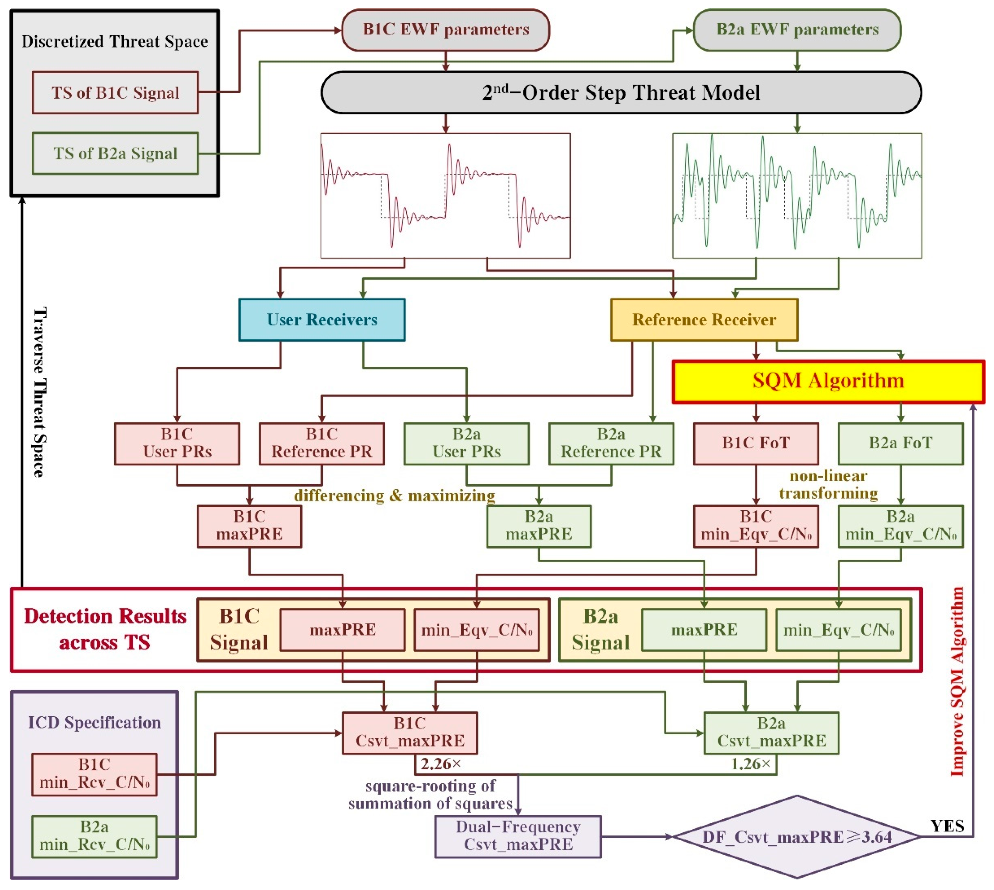
Figure 1 shows the design methodology of the SQM algorithm for BDS B1C and B2a signals.
The SQM algorithm design for BDS B1C and B2a signals operates as follows:
(1) The TS of B1C/B2a signal is discretized into tens of thousands of threat points, each of which consists of three EWF parameters. The discretization applied in this paper is given in
Table 3.
(2) Draw a threat point out of the discretized TS of B1C/B2a signal to generate the corresponding EWF by applying the 2OS-TM. The formulation of EWF-generation is based on the simulative method in Reference [
31]. As examples in
Figure 1, the EWF of B1C in red is generated with Δ = 0.05 chips,
= 15 MHz, and
= 11 MNp/s, and that of B2a in green is with Δ = 0.5 chips,
= 15 MHz, and
= 11 MNp/s. Note that the chip period of B1C signal is ten times that of the B2a signal. The black dashed lines represent the corresponding ideal rectangle waveforms, respectively.
(3) The generated EWF of the B1C/B2a signal is processed by the reference receiver and numerous user receivers. The specified receiver configurations given in
Table 4 are consistent with the specifications in Reference [
23]. Each receiver will measure a bias that is caused by the combination of signal deformation and receiver configuration. This bias is denoted as PR in
Figure 1 to represent a measured pseudorange only with differential-mode errors. The absolute difference between the Reference PR and a User PR seems to be the differential pseudo-range error experienced by this particular user. By performing this differencing process between the Reference PR and tens of User PRs, the maximum one of the tens of calculated differential pseudorange errors is the maxPRE of the threat point. The calculated maxPRE of the B1C/B2a signal should be saved in Detection Results.
(4) The refence receiver will also send the generated EWF of B1C/B2a signal to a designed SQM algorithm in the bright yellow rectangle in
Figure 1. The SQM algorithm will measure values of the defined metrics with the EWF, and then compare the measured metric values to their nominal ones against corresponding MDEs. The maximum one of the calculated ratios is designated as the figure of test (FoT) of the SQM algorithm to this threat point. The obtention of an FoT value is given by:
where
represents the number of defined metrics and the superscript nom is the abbreviation for nominal. The FoT value will be non-linearly transformed into a value of minimum equivalent carrier-to-noise ratio (min_Eqv_C/N
0). The calculated values of min_Eqv_C/N
0 for the B1C/B2a signal should be saved in Detection Results.
(5) Traverse the discretized TS of the B1C/B2a signal until the values of maxPRE and min_Eqv_C/N0 of all the threat points are obtained.
(6) Calculate the values of minimum receiving carrier-to-noise ratio (min_Rcv_C/N
0) of the B1C and B2a signals in accordance with the corresponding interface control documents (ICDs) [
25,
26] for conservativeness, given by:
where −161 dBW and −158 dBW are the minimum received power levels on ground, −0.3 dB and −0.6 dB are the correlation losses, −5.5 dB is more conservative [
1,
27] than the −3.1-dB antenna gain of the omnidirectional NovAtel GNSS-750 antenna at 5-degree elevation [
32], and −228.6 dBJ/K and 24.8 dBK are calculated with the Boltzmann constant and the operating temperature of 300 K, respectively. In addition, the operation of 100-s metric-smoothing is conventionally applied to smooth down the poorly spatially- and/or temporally-correlated code noise and multipath errors, from which a smoothing gain no lower than 4 dB is expected [
11]. Thus, the values of min_Rcv_C/N
0 of B1C and B2a signals for the design and evaluation of SQM algorithm in this paper are set to 39.2 and 40.7 dB-Hz, respectively. Note that the GEOs and inclined geosynchronous orbit satellites (IGSOs) of BDS are invisible to some other important DFMC SBASs that will be monitoring BDS signals, e.g., WAAS and EGNOS, but only medium Earth orbit satellites (MEOs). Thus, the values would be 2 dB higher for both signals [
25,
26]. However, for conservative discussions, the values of IGSOs are applied for generality.
(7) The detection result of the B1C/B2a signal consists of a group of maxPRE values and a group of min_Eqv_C/N0 values that are corresponding to the discretized TS. Consequently, the monotonically descending confidence bounds provided by the tested SQM algorithm will be obtained with ascending carrier-to-noise ratio values (C/N0) to overbound the corresponding maxPRE values. Thus, given the min_Rcv_C/N0 of the B1C/B2a signal, the value of conservative maxPRE (Csvt_maxPRE) will be found out.
(8) The errors in each of the individual SF signals will be inflated in the iono-free combinations in accordance with Equation (9). Thus, the Csvt_maxPREs of B1C and B2a signals need be multiplied by 2.26 and 1.26, respectively. Subsequently, calculate the summation of the squares of the inflated Csvt_maxPREs and then the square-root of it to reach the dual-frequency conservative maxPRE (DF_Csvt_maxPRE).
(9) According to Equation (10), compare the calculated DF_Csvt_maxPRE with 3.64 m (DFREI = 4). If the 3.64-m limit is exceeded, the tested SQM algorithm should be improved and the whole procedure shall be run again. Otherwise, the tested SQM algorithm is capable of protecting DF users against HMI induced by distorted signals, and the evaluation is accomplished.
Note that there is conventionally a reference-averaging process among the corresponding metric values from different in-view reference stations to a satellite to average down the differential-mode errors, such as thermal noise and local multipath, based on the fault-free hypothesis of satellite-free differential-mode errors. However, there exists significant uncertainties in the practical distributions and elevations of the visible stations to the same satellite. Besides, the satellite-induced elevation-dependent tracking errors ever observed in GPS SVN-49 and BDS-II signals might introduce the risks of reference-averaging invalidity [
33]. Thus, it should be emphasized that the reference-averaging gain shall not be considered in SQM algorithm design.
In order to reduce implementation complexity, some simplifications and/or optimizations might be needed, including those by simplifying the hardware implementations or reducing the number of metrics while sustaining the expected detection capability.
4. SQM Algorithm Design for BDS B1C and B2a Signals
The procedure of SQM algorithm design will be performed in this section in accordance with the design methodology proposed in
Figure 1. Since MCO-based SQM methods are commonly used in L1-only SBASs, the MCO-based baseline algorithm proposed in Reference [
11] is first applied to initialize design procedure. As the second iteration of the design procedure, a CDO-based algorithm with generally optimal configuration given in Reference [
7] is evaluated, which seems to be the CDO-based baseline algorithm. In order to seek the genuine optimal code-phase bin length for BDS B1C/B2a combination while lowering the required sampling frequency for general implementation, the operations of practicalization including the optimizations of bin length and the iterations of algorithm evaluation are performed. With the practically optimal configuration, the sensitivity of CDO-based metrics is tested to reduce the number of metrics, accounting for the computational complexity while sustaining the expected performance in meeting the ICAO requirements for CAT-I PA.
4.1. Evaluation of the MCO-Based SQM Baseline Algorithm
In order to achieve the baseline performance of the MCO-based SQM algorithm, we apply schemes with dense distributions of correlators, i.e.:
for the B1C signal, 51 correlators are utilized, which are uniformly distributed between −0.25 and +0.25 chips with 0.01-chip spacings in the CCF;
for the B2a signal, 21 correlators are utilized, which are uniformly distributed between −1.0 and +1.0 chips with 0.1-chip spacings in the CCF.
Moreover, the detection metrics are defined as:
where
is the in-phase component of an E or L correlator value, and
is that of the P correlator value. Reference [
11] states that this scheme would achieve particularly favorable SQM performance.
With the conditions of (1) the minimum received power levels on ground for BDS IGSOs; (2) the minimum receiving elevation of 5 degrees; and (3) the minimum 4-dB gain provided by the 100-s metric-smoothing operations, the considered conservative min_Rcv_C/N
0 values of B1C and B2a signals are 39.2 and 40.7 dB-Hz, respectively, as derived in
Section 3. Note that the MDEs that are theoretically used as detection thresholds in SQM algorithm design are proportional to the standard deviations of nominal values of corresponding metrics, as indicated in Equation (4). For conservativeness, the above min_Rcv_C/N
0 values are selected as the worst nominal. The expressions of variations of the metrics defined in Equation (15) are given by:
where
. Note that the expressions for diff- and sum-ratio metrics with
for the B1C signal are not given due to the definition that the correlator values of interest are only distributed between −0.25 and +0.25 chips. By square-rooting the results in Equation (16), the standard deviations of MCO-based metrics with given
will be obtained for calculating corresponding MDEs. The derivations corresponding to Equation (16) are detailed in
Appendix A.
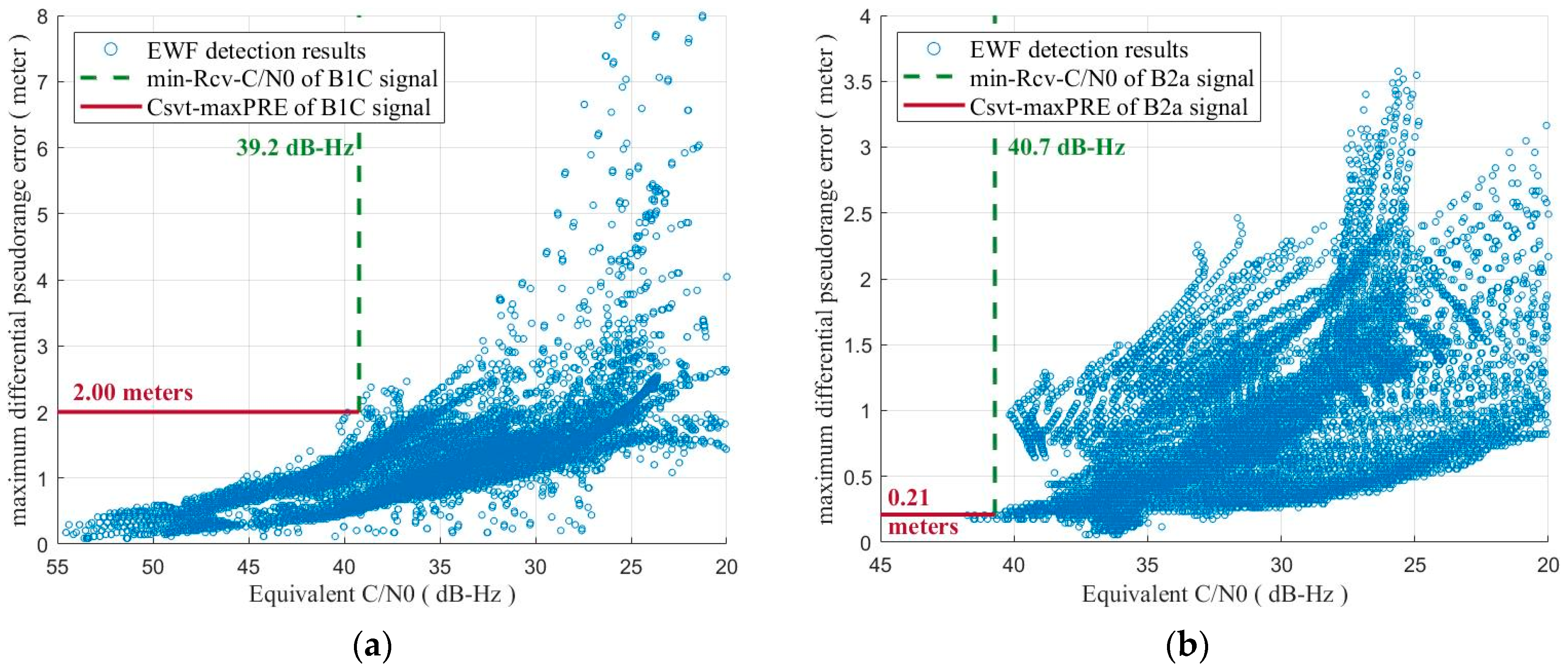
Figure 2a,b show the evaluation results of the MCO-based SQM baseline algorithm for B1C and B2a signals, respectively, where the blue scatters represent the correspondence between the min_Eqv_C/N
0 and maxPRE values of a threat point within the discretized TS, the green vertical dashed lines indicate the given min_Rcv_C/N
0 value of a signal, and the red horizontal lines give the corresponding Csvt_maxPRE value of a signal guaranteed by the SQM algorithm. As shown in
Figure 2, the DF_Csvt_maxPRE value of BDS B1C/B2a combinations guaranteed by the MCO-based SQM baseline algorithm is calculated as:
Therefore, the MCO-based SQM baseline algorithm can only provide a protection equivalent to DFREI = 5 [
13], not meeting the preset condition of DFREI-4. Since the baseline performance of MCO-based SQM is unsatisfactory, the emerging CDO-based methods will be tested.
4.2. Evaluation of the CDO-Based SQM Baseline Algorithm
Reference [
7] gives a generally optimal SQM algorithm based on CDOs for DFMC SBAS, called the SCSQM8r algorithm. The sampling frequency and the sectionalization of code-phase bins are the core influential factors of a CDO-based SQM algorithm [
7]. In this subsection, an algorithm with a sampling frequency of 72 MHz and bins of 0.025 B1-chips is evaluated to find out the relatively more advantageous performance.
The SCSQM8r algorithm applies 8 CDOs in the chip rising edges, which are denoted as CDO
1, CDO
2, …, CDO
8 serially and distributed with 0.025 B1-chip spacings symmetrically. Moreover, the 8 CDOs are directly utilized as 8 metrics, aiming to achieve the primary performance of CDO-based SQM algorithm. In the CDO-based SQM baseline algorithm discussed in this subsection, the 8 CDOs are also applied but the metrics are expanded as:
to hopefully achieve a better performance. Since the noise in a CDO is Gaussian [
7], the powers and/or the products of CDOs are not applied as metrics due to the computational complexities in theoretical derivations and/or practical operations induced by the Chi-square distribution, and the quotients of CDOs are not applied either because of the inexistence of mean and variation of Cauchy variables. The numbers of single-, dual-, triple-, and quad-CDO metrics are given by:
respectively. Therefore, the combinations of more than four CDOs are also not applied as metrics for the sake of computational complexity.
As indicated in Equation (12), a CDO is the mean of all the samples captured by the same bins of all the rising edges within a given integration period. The incorporated samples from the RF front-end output are deemed independent and identically distributed (IID) and affected by additive white Gaussian noise (AWGN) [
17]. As a consequence, the standard deviation of a CDO is affected by the standard deviation of the AWGN and the number of samples incorporated. Since the fact that neither the sampling frequency could be divided exactly by the chip rate nor rising edges are uniformly distributed in the code sequences, 8 standard deviations of the corresponding 8 CDOs must be inconsistent but tend to be identical for a longer integration period [
7]. The theoretical expression of the nominal standard deviation of a CDO is given in Reference [
7] as
where
is the double-sided pre-correlation bandwidth,
is the sampling frequency of the RF front-end output, RER is the abbreviation of rising edge rate that is a ratio from the quantity of rising edges to that of chips within one code period, and BIN is the proportion of a bin to a chip. The minimum value of
across all the PRNs is applied for conservativeness, given in Reference [
7]. The standard deviations of dual-, triple-, and quad-CDO metrics can be derived based on Equation (20).
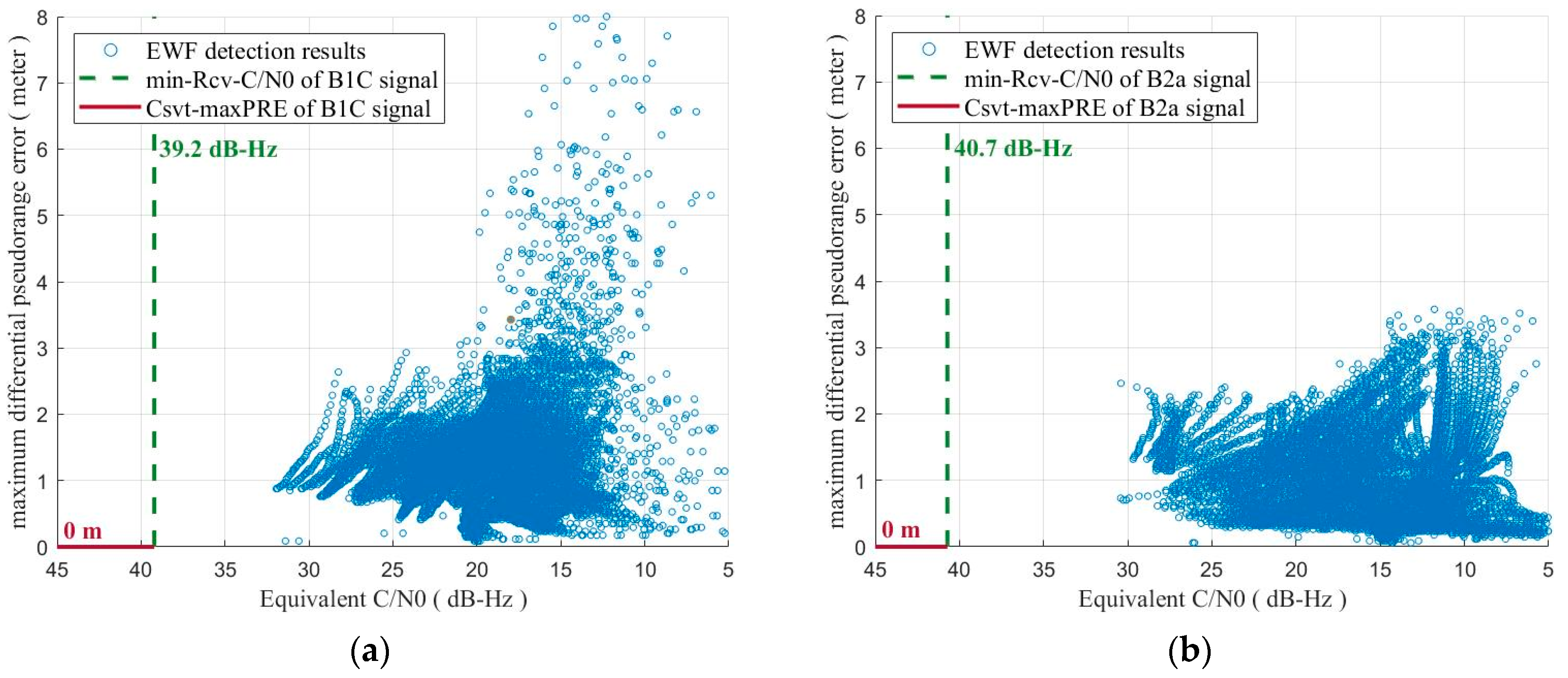
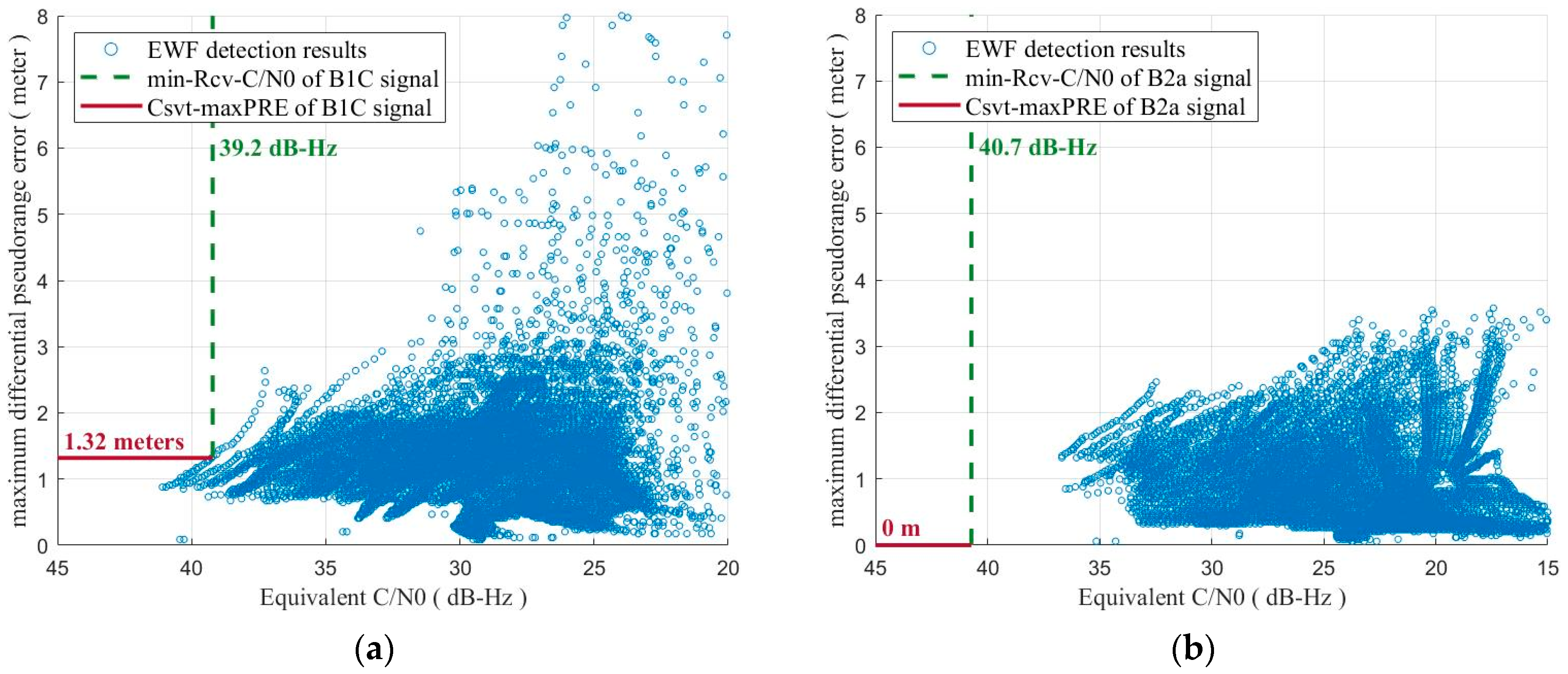
Figure 3 shows the evaluation results of the CDO-based SQM baseline algorithm with a sampling frequency of 72 MHz and bins of 0.025 B1-chips for B1C and B2a signals, respectively, where the performances are superior to those in
Figure 2. The resulted DF_Csvt_maxPRE is 0 m, indicating that a protection equivalent to DFREI = 0 [
13] could be provided. Note that the performances in
Figure 3 are also better than those given in Reference [
7] due to the application of additional dual-, triple-, and quad-CDO metrics.
Although a satisfactory performance has been achieved by the CDO-based SQM baseline algorithm, it should be noticed that a sampling frequency of 72 MHz introduces implementation complexity to the monitoring receivers. Furthermore, based on the constraint
[
7], a higher sampling frequency of the RF front-end output with the given chip sectionalization and chip rate of the monitored signal might induce correlations to the samples involved in calculating a CDO value. In addition, the length of code-phase bins is the other key influential factor in SQM design [
7]. Therefore, a practicalization of CDO-based SQM algorithm is needed for reducing complexity while providing generality.
4.3. Practicalization of CDO-Based SQM Algorithm
The practicalization of the CDO-based SQM algorithm is on the basis of the design methodology proposed in Reference [
7], including the optimizations of bin length to improve overall performance and the iterations of algorithm evaluation to lower sampling frequency, thereby reduce implementation complexity. In this design methodology, an eigen property called critical metric bias (CMB) is defined for the risky group of a signal that is the set of those threat points with maxPREs exceeding the specified MERR with the given TS discretization and receiver configurations. A CMB is expressed by:
Specifically, a CMB value, of which the provider within the Risky Group could be deemed the hardest one to detect, is particular to a given configuration of BIN and
[
7]. The MERR value will be applied in finding out the CMB values for SQM design. Provided the concept of CMB, the CMB provider of a given configuration of BIN and
will be the determinant of algorithm performance. Thus, an index named figure of merit (FoM) is further defined as:
where
is separated from the expression of
without factors of BIN and
, e.g.,
for single-CDO metrics as indicated in Equation (20). Note the differences between Equation (22) and the expression in Reference [
7]. The discussions in this paper shall not take the reference-averaging gain into consideration, thus the number of reference stations involved is ignored. The metric-smoothing improvement of 4 dB is absorbed by the
in
, where 39.2 and 40.7 dB-Hz are given for B1C and B2a signals, respectively.
The sectionalization of a chip needs some constraints in order to prevent neither losing necessary information by applying bins too fine, thus causing insufficiency, nor incorporating unnecessary information by utilizing bins too coarse, hence, inducing redundancy, because only 8 CDOs are relevant to the SQM algorithm. Reference [
7] gives a method of bin-length selection and performs among GPS L1 C/A, BDS B1C, and BDS B2a signals. The constraints have been detailed and reasoned in Reference [
7] and, hence, will not be repeated in this paper for brevity. By applying the constraints in the nominal domain, distortion domain, and rigid domain, given by:
the range of bin-length selection for B1C signal is obtained by the intersection as:
for which the fractional form is expressed as:
where the ratio 68.27% and the featured length
and
, as defined in Reference [
7], are measured in the simulated chip rising edge filtered by a 6th-order Butterworth filter, and the range of
that is the frequency of damped oscillation in the 2OS-TM is given in
Table 2. The chip period of the B2a signal is one tenth of that of the B1C signal, i.e., 4 bins with a length of 0.025 B1-chips will fulfill a B2 chip since 8 CDOs symmetric about the rising edge are applied. Thus, to the portion of
in Equation (24), a B2a code needs more than one consecutive −1 chips followed by the same number of consecutive +1 chips to correspond. Furthermore, accounting for the fact that a chip or the whole of the considered consecutive −1 and/or +1 chips should be sectionalized into integer bins, the range of bin-length selection for B1C signal in Equation (25) could be transformed to that for B2a signal as:
where the captions of single-, dual-, and triple-chip indicate the situations of (−1,+1), (−1,−1,+1,+1), and (−1,−1,−1,+1,+1,+1), respectively. The quad-chip situation is not needed according to Equation (24).
On the other hand, the sampling frequency of RF front-end output also needs some constraints. Given the constraint for bin-length selection in Equation (25), the constraint
to prevent correlation among samples in measuring CDOs, the B1C chip rate of 1.023 Mcps, and the Nyquist frequency according to the specified pre-correlation bandwidth of reference receiver in
Table 4, the considered range for sampling frequency is from 24 MHz to 72 MHz.
4.3.1. Optimal Bin Length with Equal MERRs
Given the MERR of 3.64 m in Equation (8) for BDS B1C/B2a combinations, the biases of each SF signal will be expressed as
and
, respectively. Assuming that
, the maximum allowable
, i.e., the MERRs for the individual SF signals in DF applications, shall be given by:
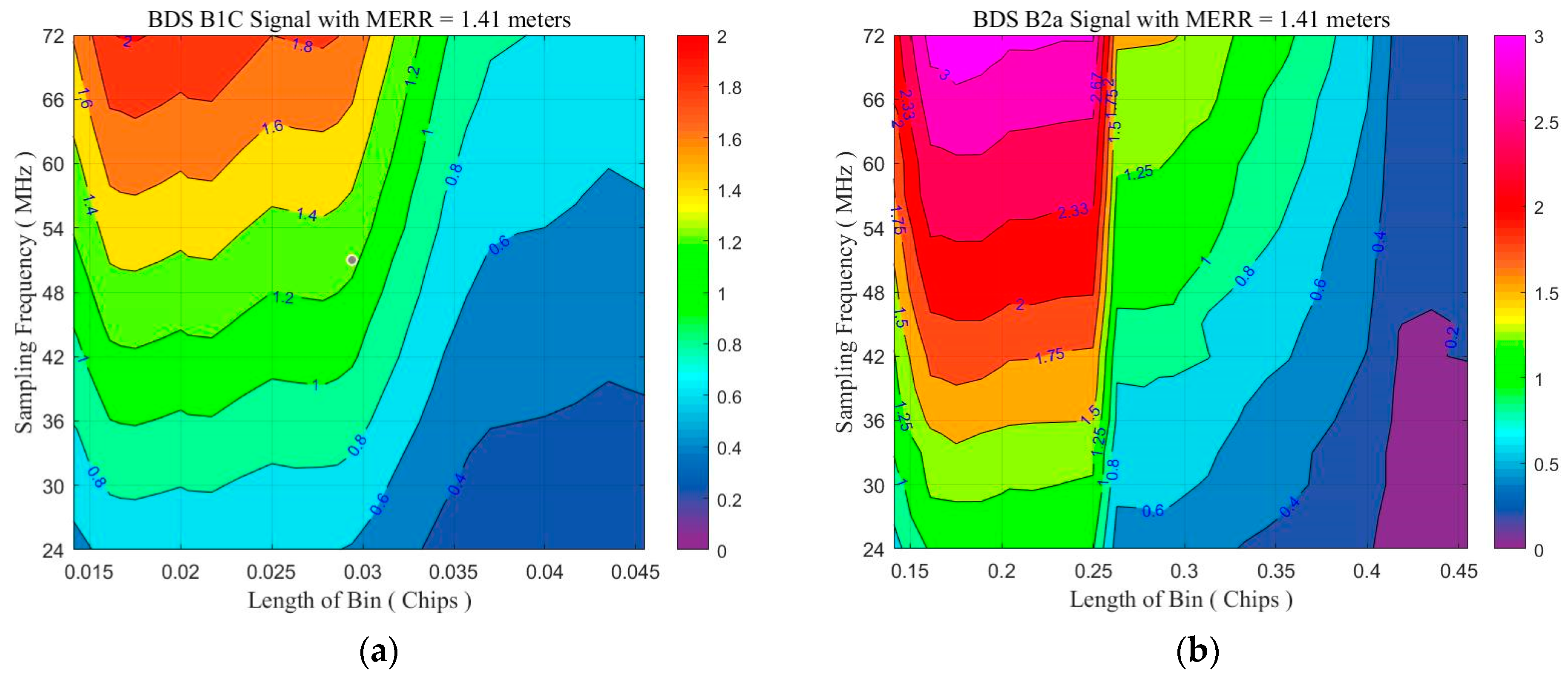
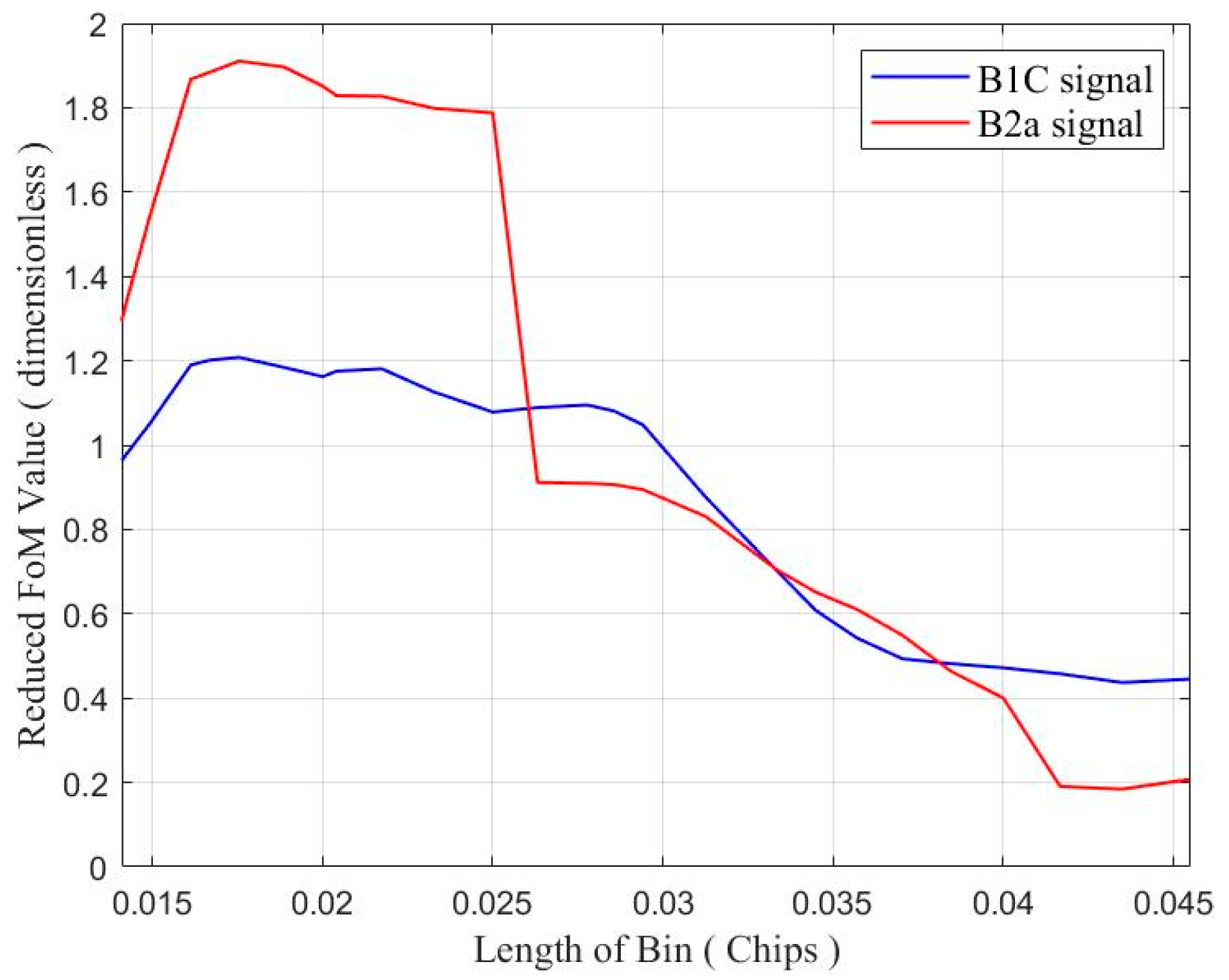
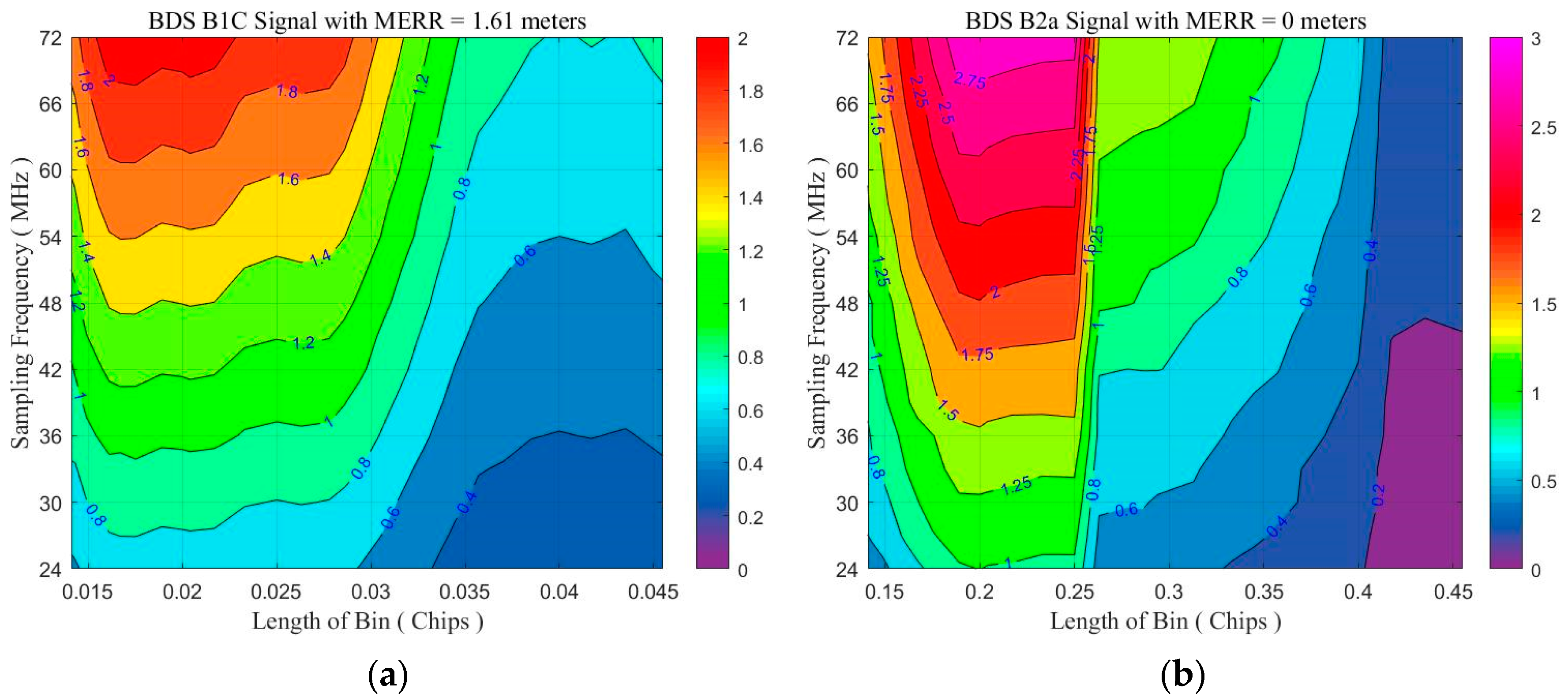
Massive simulations are performed across the ranges of BIN and
to obtain the FoM values.
Figure 4a,b show the FoM contours of B1C and B2a signals, respectively, with the 1.41-m MERR given in Equation (27). The portions with FoM values not lower than unity indicate satisfactory performance, while the rest need further examination. With any given BIN value, the FoM values are positively correlated with the
values for most of the contours, being consistent with the FoM expression in Equation (23). However, with any given
value, the trends of FoM values are not monotonic about the BIN values. Note that
might not be critically identical across the considered range of
but have little impact according to the calculation of CDOs in Equation (12). Thus, the contours in
Figure 4 are reduced vertically with the weights corresponding to
, e.g., a weight of
for a contour value of
= 72 MHz with the discretization of 72:−3:24 MHz in simulations.
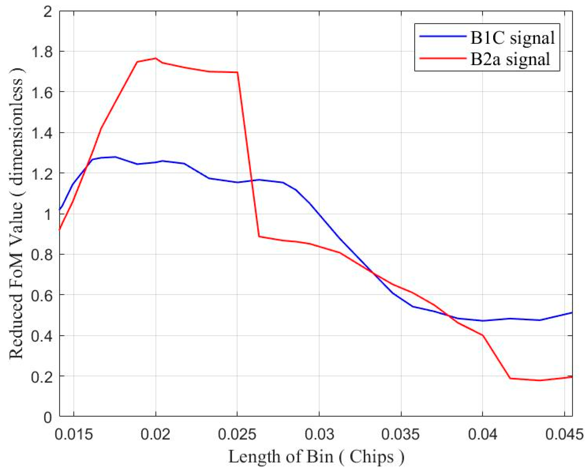
The results of contour reduction are shown in
Figure 5. The best performance with the B1C signal could be achieved at the bin-length of
B1-chips. This value is nearer to
B2-chips than to
B2-chips. Correspondingly, the reduced FoM value at
B1-chips for the B1C signal is larger than that at
B1-chip. Moreover, the FoM value of the B2a signal at either
B2-chip or
B2-chips, or even the virtual
B2-chip, is beyond unity with the lowest
of 24 MHz, as shown in
Figure 4b. Therefore, the optimal code-phase bin length is temporarily determined as
B1-chips or 16.292 nanoseconds per bin, being inconsistent with the result in Reference [
7] where three representative signals, i.e., GPS L1 C/A, BDS B1C, and BDS B2a, are involved.
Given the temporarily optimal code-phase bin length of
B1-chips, the considered lowest
of 24 MHz should be evaluated, in order to reduce implementation complexity. The Csvt_maxPRE values of 1.24 m and 0.59 m, respectively, are obtained, thereby a DF_Csvt_maxPRE of 2.90 m corresponding to DFREI = 4 [
13] is achieved. Moreover, the performance margins are about 0.5 and 4.3 dB, respectively, i.e., if the preset min_Rcv_C/N
0 values of 39.2 and 40.7 dB-Hz were virtually reduced to as low as 38.7 and 36.4 dB-Hz, respectively, the performance of a protection equivalent to DFREI-4 would still sustain.
The configuration with an of 24 MHz and bin length of B1-chips has been evaluated satisfactory under the requirements of DFMC SBAS and practical with low implementation complexity. However, there might still be some optimizations to exploit.
4.3.2. Optimal Bin Length with Unequal MERRs
Since the FoM values of the B2a signal at
,
, and
B2-chips with 24 MHz are beyond unity as shown in
Figure 4b, the MERR for the B2a signal is radicalized as 0 m, as indicated in
Figure 3b. Correspondingly, the MERR for the B1C signal is loosened as
m. The new contours are shown in
Figure 6.
The contour values in
Figure 6a are slightly higher than those in
Figure 4a, i.e., +0.0452 in weighted average. Meanwhile, the contour values in
Figure 6b are correspondingly lower than those in
Figure 4b, i.e., −0.1336 in weighted average. More specifically for the temporarily optimal code-phase bin length, i.e.,
B1-chip or
B2-chip, the weighted average differences are +0.0738 and −0.4637, respectively. While for the adjacent bin length of
B1-chip or
B2-chip, the average differences are +0.0898 and −0.0866, respectively. Thus, this unequal-MERR scheme pays a larger B2a performance loss in exchange for a far smaller B1C performance gain with the temporarily optimal code-phase bin length. However, the situation with a bin length of
B1-chip or
B2-chip is nearly balanced. Again, we reduce the contours vertically to get the weighted FoM values, shown in
Figure 7.
Figure 7 tells that the curve values at
,
, and
B1-chips are 1.2750, 1.2789, and 1.2522, respectively, for the B1C signal. However, the values for the B2a signal vary significantly. Thus, the optimal code-phase bin length moves forward to
B1-chips or 19.550 nanoseconds per bin, temporarily. This new temporarily optimal value will be evaluated against the considered lowest
of 24 MHz to find whether the CDO-based SQM algorithm is eligible.
With an
of 24 MHz and bin length of 0.020 B1-chips, the DF_Csvt_maxPRE of BDS B1C/B2a combinations guaranteed by the CDO-based SQM algorithm is calculated as:
indicating that a protection equivalent to DFREI = 4 [
13] could be provided. The performance margins are about 0.9 and 4.0 dB, respectively.
The performances of the configuration of 1/60-B1-chip bins (cfg-1) and the configuration of 1/50-B1-chip bins (cfg-2) with an of 24 MHz are compared as follows:
cfg-1 achieves a lower DF_Csvt_maxPRE value (2.90 m) than cfg-2 does (2.98 m), but the values are comparable;
cfg-1 provides a total performance margin (4.8 dB) near cfg-2 does (4.9 dB), but the margin for the B1C signal provided by cfg-2 (0.9 dB) is about twice the value provided by cfg-1 (0.5 dB).
Considering the balance between the SQM performance for the two signals and the protection enhancement for the main ranging signal of BDS, i.e., the B1C signal, we decide to choose 1/50-B1-chip or 1/5-B2-chip bins as the optimal value.
To sum up, the CDO-based SQM algorithm with the optimal code-phase sectionalization of 0.020 B1-chips or 0.20 B2-chips identically can provide the required protection that is equivalent to DFREI = 4 with a sampling frequency of the RF front-end output as low as 24 MHz.
4.4. Simplification of CDO-Based SQM Algorithm
As shown in
Figure 4 and
Figure 6, the contour values corresponding to different BINs vary violently, given a fixed
. The sensitivities of different CDOs to an EWF are closely relevant to the length of bins, due to the modeled fluctuations defined in the 2OS-TM. Reference [
7] gives a demonstration to examine the sensitivities of CDOs. In this study, 848 metrics are defined for a CDO-based SQM algorithm in Equation (18). Similarly, the sensitivities of these CDO-based metrics could be examined to simplify the algorithm.
With full metrics, the algorithm could provide DFREI-4 level protection with 0.9- and 4.0-dB performance margins, respectively, as shown in
Figure 8. Thus, we examine the sensitivities of metrics with the B1C signal, aiming to combine the detection capabilities of several metrics to hold the 1.61-m MERR limit. Accordingly, the B2a signals applies the same group of metrics as the B1C signal does to keep algorithm consistency.
(1) Ten metrics are picked out to preserve the performance in
Figure 8a, including:
(10) ,
(5) ;
(3) ,
(7) ;
(6) ,
(9) ,
(1) .
The indices ahead of the metrics represent the ranks of sensitivities, e.g., (1) means the most sensitive metric while (10) means the least sensitive one among the ten. This group of ten metrics can hold the 0.9-dB performance margin and 1.32-m Csvt_maxPRE for the B1C signal, while may consume 1.4 dB of the 4-dB performance margin for the B2a signal.
(2) The tenth metric, , is removed for another evaluation. This group of nine metrics performs equivalently as the ten-metric group does.
(3) Moreover, the ninth metric, , is removed for further evaluation. This group of eight metrics consumes 0.4 dB of the 0.9-dB performance margin for the B1C signal.
(4) However, if the eighth metric,
, is removed, the Csvt_maxPRE values of B1C and B2a signals would increase to about 3.05 and 0.53 m, respectively, meaning a 6.93-m DF_Csvt_maxPRE equivalent to a protection of DFREI = 7 [
13].
Therefore, the eight-metric group is the result of algorithm simplification that we suggest for BDS B1C/B2a combinations toward DFMC SBAS. The algorithm is summarized in
Table 5. This algorithm is named Chip Domain Signal Quality Monitoring with 8 CDOs in rising-edges (CDSQM8r).
5. Conclusions
BDSBAS is under construction and has formed the initial operational capability by 2022 [
3]. In 2025, the DFMC service must be playing a significant role in BDSBAS services toward civil aviation and many other life-safety fields. The integrity monitoring architecture is important for an SBAS in enhancing GNSS integrity, where signal deformation would be the largest source of ranging uncertainty in dual-frequency applications. This paper systematically studies the SQM for BDS B1C/B2a civilian signals and proposes the design methodology for SQM algorithm, which can be seen as a paradigm for the DF civilian signals of any GNSS core constellation under given TM, TS, and performance requirements, which, thus, can easily be extended in the name of DFMC.
The traditional MCO-based and the emerging CDO-based SQM baseline algorithms are fully evaluated and discussed. Moreover, in order to promote overall performance while preserving a lower implementation complexity, a whole design procedure of a CDO-based algorithm is performed, including the operations of practicalization and simplification. In the practicalizing operations, the optimal code-phase bin length is achieved with low sampling frequency of the RF front-end output. While in the simplifying operations, the sensitivity of metrics is examined, hence, the number of necessary metrics are sharply reduced for computational complexity. Finally, an algorithm named CDSQM8r is proposed for BDS B1C/B2a signals.
The CDSQM8r algorithm proposed In this paper could be considered as an effective candidate of DF SQM in the developing BDSBAS and other new generation DFMC SBASs for BDS DF civilian signals. Furthermore, once provided the standard 2OS-TM, the specific TSs, and the requirements equivalent to that of CAT-I PA in civil aviation, other algorithms might be worked out for the combinations of GPS L1C/A/L5-Q, GLONASS L1OCd/L3OC, and Galileo E1-C/E5a-Q. After checking the compatibility and interoperability of these potential algorithms, the generic CDO-based SQM algorithm towards DFMC SBAS would be reached.


