

Characterization of Operational Vibrations of Steel-Girder Highway Bridges via LiDAR


Abstract
:1. Introduction
2. Objectives and Approach
3. Field Data Collection
3.1. Observation from an Operating Highway Bridge
3.1.1. Temporal Frequency during the Field Data Collection
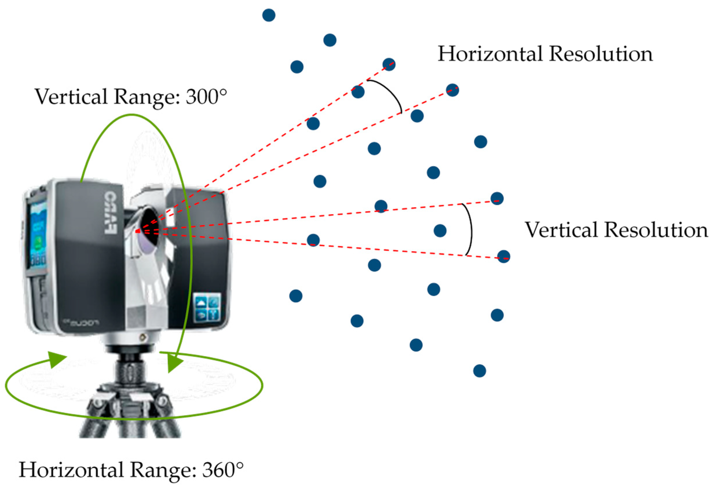
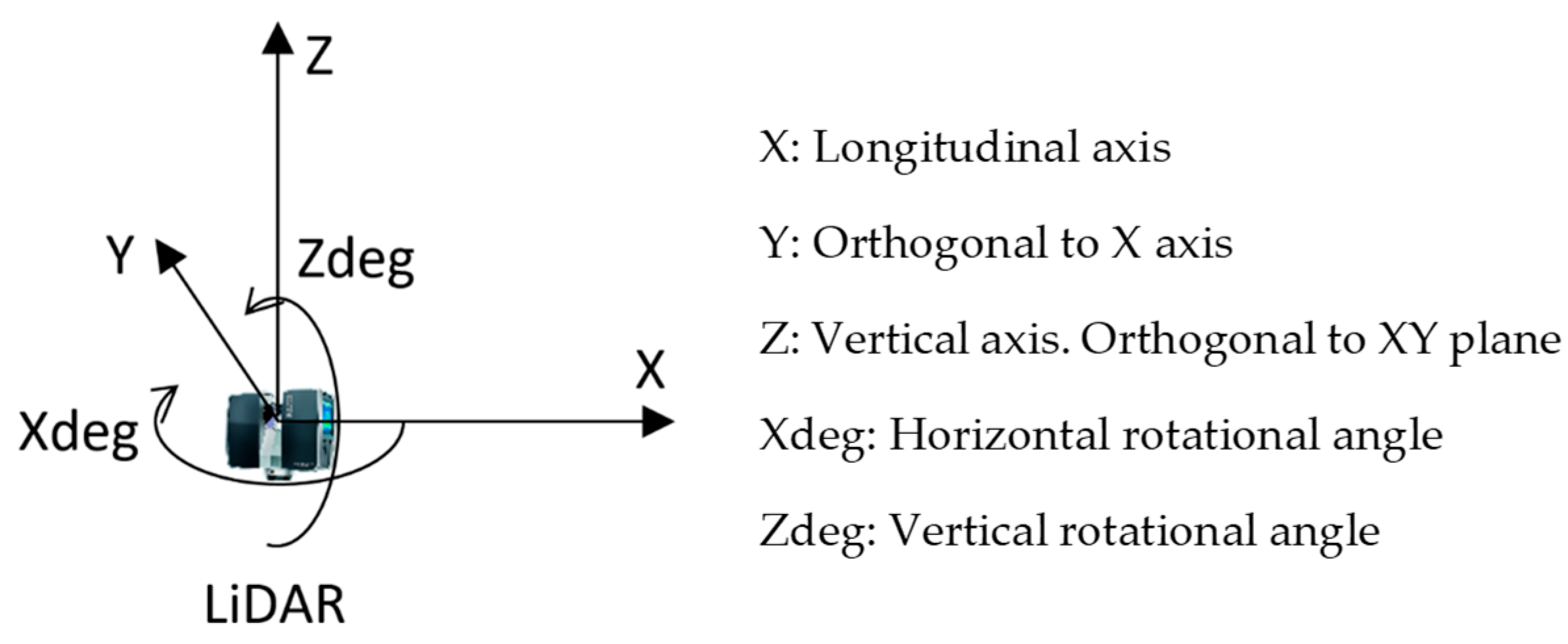
3.1.2. Angular Frequency during Field Data Collection
3.1.3. Measurement of the Bridge Frequency of Vibrations
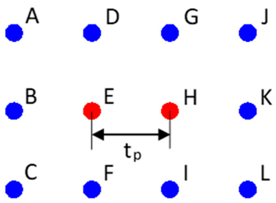
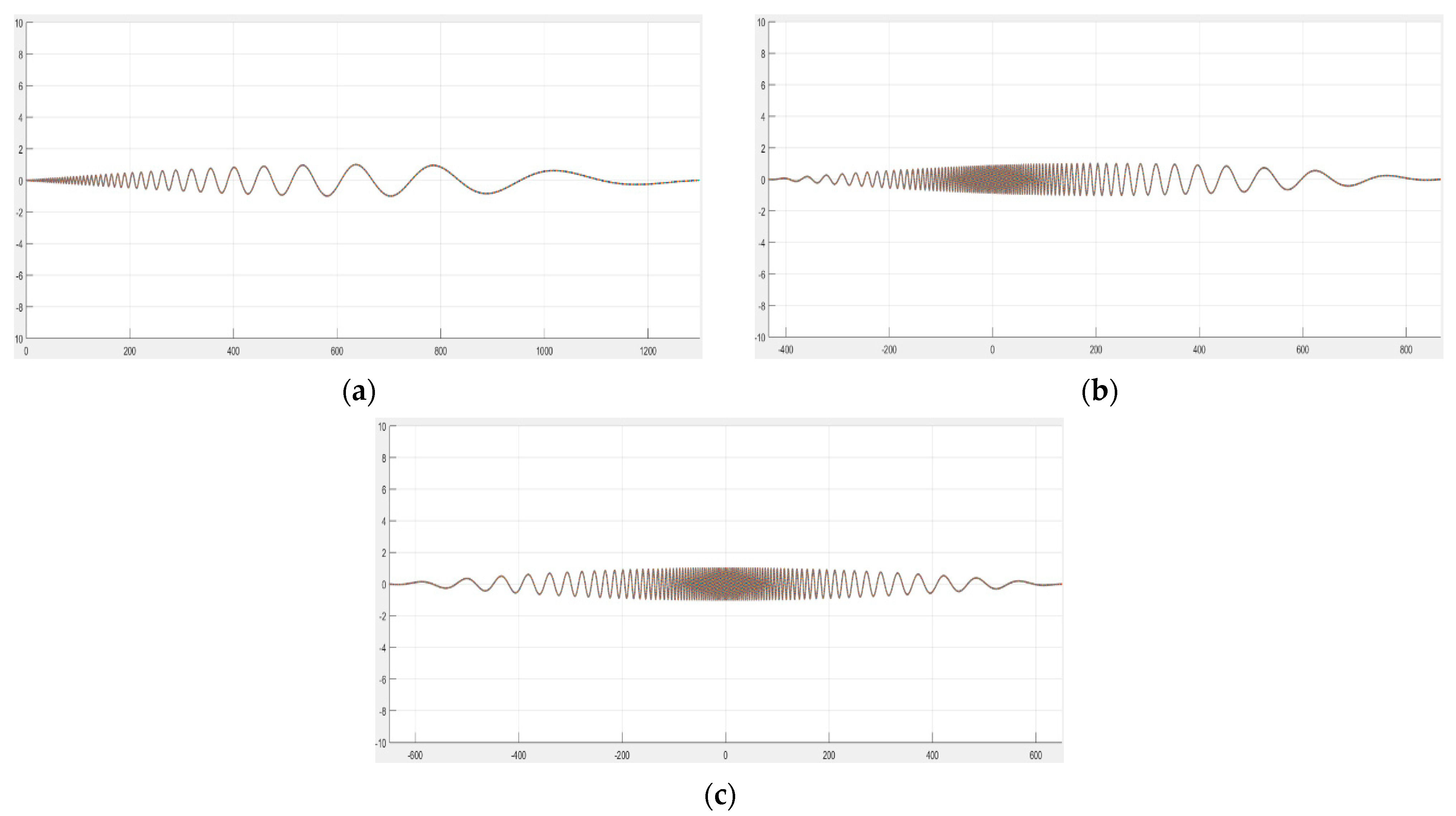
- Calculate the angular distance (Distang) between the two low points (of a ripple), considering the LiDAR’s location following Equation (3). X and Y are the coordinates of the selected data points.
- Calculate the period between ripples (TR), which is the time, in seconds, between the occurrence of two consecutive low points, following Equation (4).
- Calculate the bridge frequency of vibration (fo), following Equation (5).
4. Field Data Analysis and Results
5. Numerical Modeling
- Calculate the Xdeg of each point with respect to the scanner and assign a distance alpha. Alpha is the longitudinal location of the point within the plate (see Equation (8)).
- Calculate the Zdeg of each point with respect to the scanner and assign a distance beta. Beta is the transverse distance of the point within the plate (see Equation (9)).
- Assign an ID to each point of the point cloud, based on the scanner rotating sequence, assuming the scanner rotates forward and clockwise. The point ID (pointID) was assigned based on the following code:
- zcover = 360; %Vertical degrees covered by the scanner.ptsCicle = round((zcover/(Deg)),0); %Number of points of scanner revolution.for i = 1:size(beta,1)for j = 1:size(beta,2)pointID(i,j) = (i − 1)+ptsCicle*(j − 1);endend
- Finally, the algorithm needed a shape function (Equation (10)), a time assigned to each point (Equation (11)) and the natural frequency that was previously calculated to calculate the vertical displacement for each point, as presented in Equation (12).
- (1)
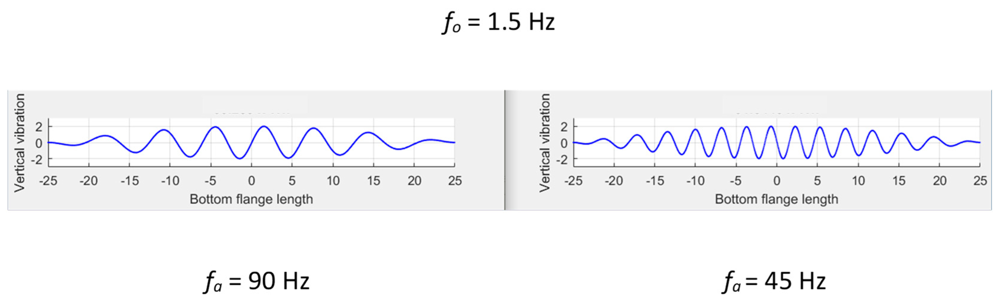
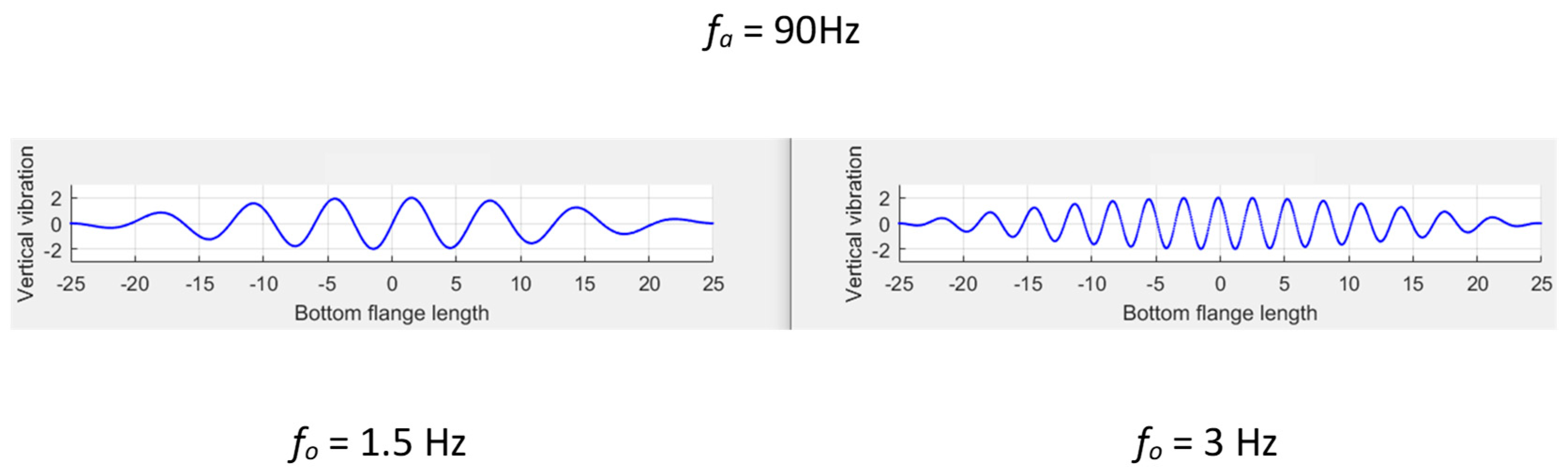
- As the resolution increases (the angular distance between two consecutive points), there will be an increase in the angular frequency. This will increase the distance between ripples for a given vibration frequency.
- (2)
- As the temporal frequency decreases, there will be a decrease in the angular frequency. This will decrease the distance between ripples for a given vibration frequency.
6. Conclusions
- (1)
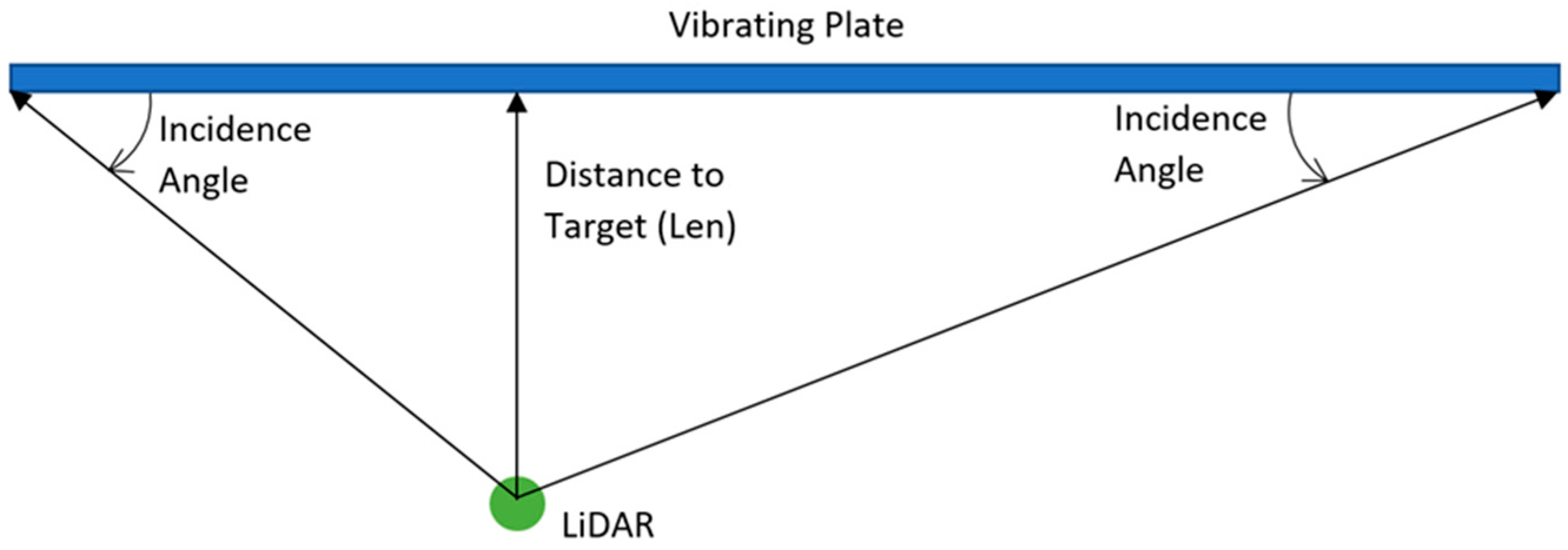
- Step 1—Select the maximum distance between the scanner and the object being scanned from Table 8 (reproduced below), ensuring that the amplitude of vibration is at least 1.5 times the manufacturer-specified accuracy.
- (2)
- Step 2—Select the angular frequency to be between 3.5 and 13 degrees/s and then use Table 9 to select the desired temporal frequency to ensure no aliasing will occur. The criteria to avoid aliasing (as mentioned in the conclusions) were taken as a minimum of eight times the frequency of the vibrating object.
- (3)
- Step 3—Based on the results from Steps 1 and 2, use Table 10 to estimate the amount of time per scan, based on the initial Step Size and Temporal Frequency.
Author Contributions
Funding
Data Availability Statement
Conflicts of Interest
References
- ASCE. 2021 Infrastructure Report Card; ASCE: Reston, VA, USA, 2021. [Google Scholar]
- Kim, J.; Gucunski, N.; Dinh, K. Deterioration and Predictive Condition Modeling of Concrete Bridge Decks Based on Data from Periodic NDE Surveys. Infrastruct. Syst. 2019, 25, 04019010. [Google Scholar] [CrossRef]
- Kijewski-Correa, T.; Haenggi, M.; Antsaklis, P. Wireless Sensor Networks for Structural Health Monitoring: A Multi-Scale Approach. In Proceedings of the Structures Congress 2006: 17th Analysis and Computation Specialty Conference, St. Louis, MO, USA, 18–21 May 2006. [Google Scholar] [CrossRef]
- Niezrecki, C.; Baqersad, J.; Sabato, A. Digital Image Correlation Techniques for NDE and SHM; Handbook of advanced non-destructive evaluation; Springer: Berlin/Heidelberg, Germany, 2018. [Google Scholar] [CrossRef]
- FARO Focus Laser Scanner; FARO Technologies: Lake Mary, FL, USA, 2020.
- Young, C.B. Assessing Lidar Elevation Data for KDOT Applications. No. K-TRAN: KU-10-8. Kansas DoT. Bur. Mater. Res. 2013. [Google Scholar]
- Meral, C. Evaluation of Laser Scanning Technology for Bridge Inspection; Drexel University: Philadelphia, PA, USA, 2011. [Google Scholar]
- Arbi, A.; Ide, K. The Application of Terrestrial Laser Scanner Surveys for Detailed Inspection of Bridges. In Proceedings of the 7th Australian Small Bridges Conference, Melbourne, Australia, 23–24 November 2015. [Google Scholar]
- Hoensheid, R. Evaluation of Surface Defect Detection in Reinforced Concrete Bridge Decks Using Terrestrial Lidar; Structural Materials Technology Conference, American Society for Nondestructive Testing; Michigan Technological University: Houghton, MI, USA, 2012. [Google Scholar]
- Liu, W. Terrestrial LiDAR-based bridge evaluation. Doctoral Dissertation, The University of North Carolina at Charlotte. Diss. Abstr. Int. 2010, 71. [Google Scholar]
- Cha, G.; Sim, S.-H.; Park, S.; Oh, T. LiDAR-Based Bridge Displacement Estimation Using 3D Spatial Optimization. Sensors 2020, 20, 7117. [Google Scholar] [CrossRef] [PubMed]
- Neitzel, F.; Resnik, B.; Weisbrich, S.; Friedrich, A. Vibration monitoring of bridges. Reports of Geodesy. 2011, pp. 331–340. Available online: file:///C:/Users/MDPI/Downloads/Vibration_monitoring_of_bridges.pdf (accessed on 22 December 2022).
- Dubbs, N.C.; Moon, F.L. Assessment of Long-Span Bridge Performance Issues through an Iterative Approach to Ambient Vibration–Based Structural Identification. J. Perform. Constr. Facil. 2016, 30, 5. [Google Scholar] [CrossRef]
- Malekjafarian, A.; Martinez, D.; Obrien, E. The Feasibility of Using Laser Doppler Vibrometer Measurements from a Passing Vehicle for Bridge Damage Detection. Shock. Vib. 2018, 2018, 9385171. [Google Scholar] [CrossRef]
- Dai, K.; Boyajian, D.; Liu, W.; Chen, S.E.; Scott, J.; Schmieder, M. Laser-based field measurement for a bridge finite-element model validation. J. Perform. Constr. Facil. 2014, 28, 04014024. [Google Scholar] [CrossRef]
- Roberts, G.W.; Meng, X.; Dodson, A.H. The use of kinematic GPS and triaxial accelerometers to monitor the deflections of large bridges. In Proceedings of the 10th International Symposium on Deformation Measurement, FIG, Orange, CA, USA, 19–22 March 2001; pp. 19–22. [Google Scholar]
- Ali, A.; Sandhu, T.Y.; Usman, M. Ambient Vibration Testing of a Pedestrian Bridge Using Low-Cost Accelerometers for SHM Applications. Smart Cities 2019, 2, 20–30. [Google Scholar] [CrossRef]
- Abedin, M.; Mehrabi, A.B. Health Monitoring of Steel Box Girder Bridges Using Non-Contact Sensors; Structures; Elsevier: Amsterdam, The Netherlands, 2021; Volume 34. [Google Scholar]
- Trias, A.; Yu, Y.; Gong, J.; Moon, F.L. Supporting quantitative structural assessment of highway bridges through the use of LiDAR scanning. Struct. Infrastruct. Eng. 2022, 18, 824–835. [Google Scholar] [CrossRef]
- Morassi, A.; Tonon, S. Dynamic Testing for Structural Identification of a Bridge. J. Bridg. Eng. 2008, 13, 573–585. [Google Scholar] [CrossRef]
- Barker, M.; Staebler, J. Serviceability Limits and Economical Steel Bridge Design (Fhwa-Hif-11-044); Federal Highway Administration (FHWA): Philadelphia, PA, USA, 2011. [Google Scholar]
- Malekjafarian, A.; Obrien, E.J. Identification of Bridge Mode Shapes Using Short Time Frequency Domain Decomposition of the Responses Measured in A Passing Vehicle. Eng. Struct. 2014, 81, 386–397. [Google Scholar] [CrossRef] [Green Version]


| Resolution (°) | Temporal Frequency ft (Points/s) | Angular Frequency fa (Degrees/s) |
|---|---|---|
| 0.035 | 24 | 0.805 |
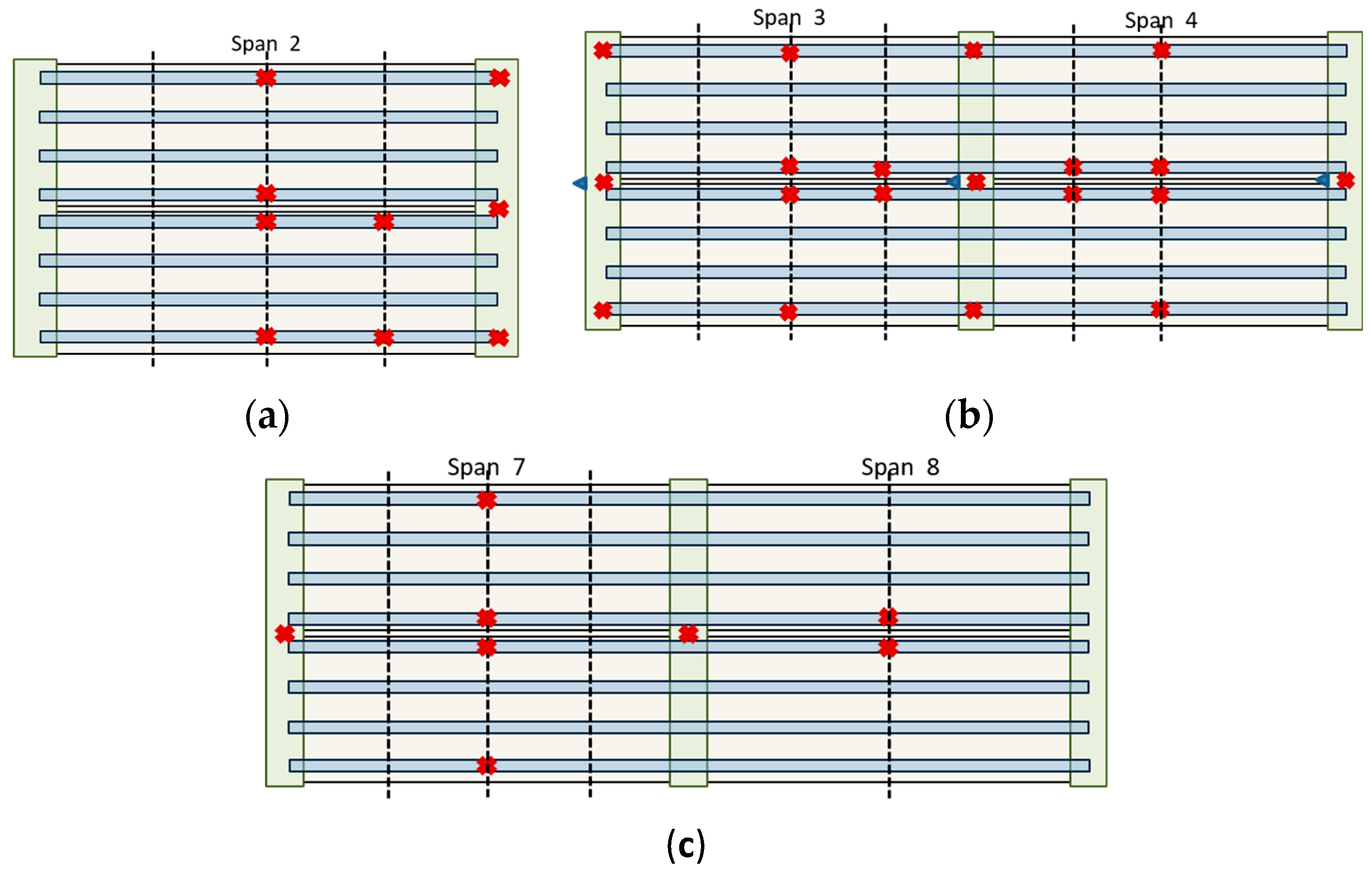
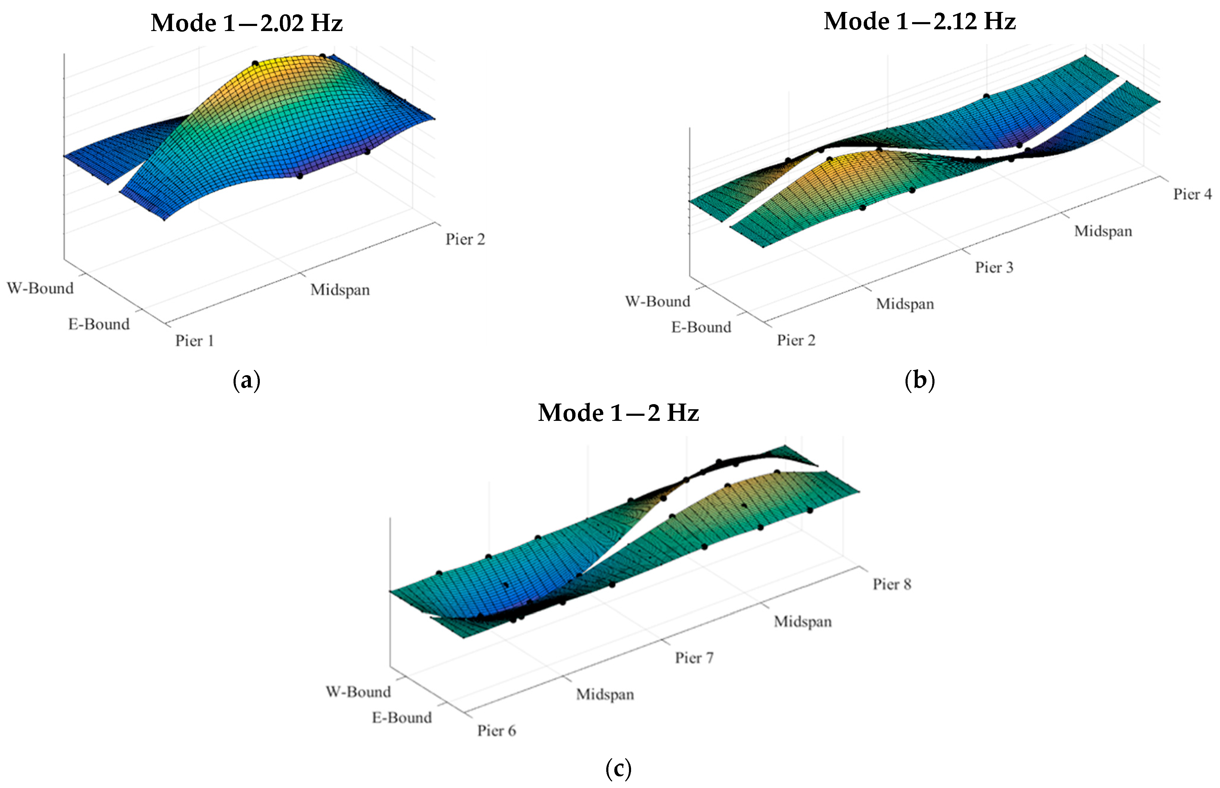
| Span Number | Average Angular Distance Distang (°) | Standard Deviation Distang (°) | Ripple Period TR (s) | Frequency of Vibration fo from the LiDAR Data (Hz) | Frequency of Vibration fo from the Dynamic Test (Hz) |
|---|---|---|---|---|---|
| 2 | 0.42 (±0.03) | 0.03 | 0.51 (±0.04) | 1.98 ± 0.13 (−1.98%) | 2.02 |
| 3 and 4 | 0.35 (±0.06) | 0.04 | 0.43 (±0.08) | 2.35 ± 0.42 (10.8%) | 2.12 |
| 7 | 0.40 (±0.09) | 0.05 | 0.48 (±0.10) | 2.07 ± 0.49 (3.5%) | 2.00 |
| 8 | 0.36 (±0.03) | 0.01 | 0.43 (±0.04) | 2.30 ± 0.22 (15.0%) | 2.00 |
| Mode Shape | Span 2 | Span 3–4 | Span 7–8 |
|---|---|---|---|
| 1 | 2.02 | 2.12 | 2.00 |
| 2 | 2.12 | 2.47 | 2.03 |
| 3 | 2.62 | 2.92 | 2.10 |
| 4 | 2.72 | 3.53 | 2.44 |
| 5 | 3.13 | 5.04 | 2.51 |
| 6 | 3.88 | 5.55 | 2.54 |
| 7 | 4.29 | 5.85 | 2.83 |
| 8 | 5.04 | 7.26 | 2.93 |
| Parameter Name | Description | Symbol | Unit |
|---|---|---|---|
| Length | Length of the span being simulated | L | cm |
| Width | Width of the typical girder bottom flange | b | cm |
| Stiffness | Flexural Stiffness of the bridge | K | kg/cm |
| Mass | Total mass of the bridge | m | kg |
| Acceleration multiplier | Acceleration multiplier to increase the amplitude of vibration | U | Unitless |
| Parameter Name | Description | Symbol | Unit |
|---|---|---|---|
| Resolution | Angular distance between two consecutive points. | Deg | Degrees |
| Distance to Target | Perpendicular distance between the scanner and plate | Len | cm |
| Temporal Frequency | Number of scanner revolutions per second | ft | rev/s |
| Scanner Longitudinal Location | Location of the scanner with respect to the longitudinal direction of the plate | LongLoc | cm |
| Scanner Transverse Location | Location of the scanner with respect to the transverse direction of the plate | TranLoc | cm |
| LiDAR’s Temporal Frequency: 90 Hz (20 × 1st Mode Frequency) | LiDAR’s Temporal Frequency: 45 Hz (10 × 1st Mode Frequency) |
|---|---|
 Resolution: 0.009° Angular frequency: 0.801 Deg/s |  Resolution: 0.009° Angular frequency: 0.396 Deg/s |
 Resolution: 0.09° Angular frequency: 8.01 Deg/s |  Resolution: 0.09° Angular frequency: 3.96 Deg/s |
 Resolution: 0.9° Angular frequency: 80.1 Deg/s |  Resolution: 0.9° Angular frequency: 39.6 Deg/s |
| Parameters | Ripple Pattern |
|---|---|
| Resolution: 0.009° fa: 26.1 Len: 9.14 m. |  |
| Resolution: 0.009° fa: 26.9 Deg/s Len: 91.4 m. |  |
| Resolution: 0.009° fa: 26.9 Deg/s Len: 914 m. |  |
| LiDAR’s Step Size (Degrees) | ||||||||||
|---|---|---|---|---|---|---|---|---|---|---|
| 0.009 | 0.018 | 0.035 | 0.040 | 0.070 | 0.088 | 0.140 | 0.175 | 0.280 | ||
| Distance to Target (meters) | 1 | 0.028 | 0.057 | 0.110 | 0.126 | 0.220 | 0.276 | 0.440 | 0.550 | 0.880 |
| 2 | 0.057 | 0.113 | 0.220 | 0.251 | 0.440 | 0.553 | 0.880 | 1.100 | 1.759 | |
| 3 | 0.085 | 0.170 | 0.330 | 0.377 | 0.660 | 0.829 | 1.319 | 1.649 | 2.639 | |
| 4 | 0.113 | 0.226 | 0.440 | 0.503 | 0.880 | 1.106 | 1.759 | 2.199 | 3.519 | |
| 5 | 0.141 | 0.283 | 0.550 | 0.628 | 1.100 | 1.382 | 2.199 | 2.749 | 4.398 | |
| 6 | 0.170 | 0.339 | 0.660 | 0.754 | 1.319 | 1.659 | 2.639 | 3.299 | 5.278 | |
| 7 | 0.198 | 0.396 | 0.770 | 0.880 | 1.539 | 1.935 | 3.079 | 3.848 | 6.158 | |
| 8 | 0.226 | 0.452 | 0.880 | 1.005 | 1.759 | 2.212 | 3.519 | 4.398 | 7.037 | |
| 9 | 0.254 | 0.509 | 0.990 | 1.131 | 1.979 | 2.488 | 3.958 | 4.948 | 7.917 | |
| 10 | 0.283 | 0.565 | 1.100 | 1.257 | 2.199 | 2.765 | 4.398 | 5.498 | 8.797 | |
| 20 | 0.565 | 1.131 | 2.199 | 2.513 | 4.398 | 5.529 | 8.796 | 10.99 | 17.59 | |
| 30 | 0.848 | 1.696 | 3.299 | 3.770 | 6.597 | 8.294 | 13.19 | 16.49 | 26.39 | |
| 40 | 1.131 | 2.262 | 4.398 | 5.027 | 8.796 | 11.05 | 17.59 | 21.99 | 35.18 | |
| 50 | 1.414 | 2.827 | 5.498 | 6.283 | 10.99 | 13.82 | 21.99 | 27.48 | 43.98 | |
| 60 | 1.696 | 3.393 | 6.597 | 7.540 | 13.19 | 16.58 | 26.38 | 32.98 | 52.77 | |
| 70 | 1.979 | 3.958 | 7.697 | 8.796 | 15.39 | 19.35 | 30.78 | 38.48 | 61.57 | |
| 80 | 2.262 | 4.524 | 8.796 | 10.05 | 17.59 | 22.11 | 35.18 | 43.98 | 70.37 | |
| 90 | 2.545 | 5.089 | 9.896 | 11.31 | 19.79 | 24.88 | 39.58 | 49.48 | 79.16 | |
| 100 | 2.827 | 5.655 | 10.99 | 12.56 | 21.99 | 27.64 | 43.98 | 54.97 | 87.96 | |
| 110 | 3.110 | 6.220 | 12.09 | 13.82 | 24.19 | 30.41 | 48.38 | 60.47 | 96.762 | |
| 120 | 3.393 | 6.786 | 13.19 | 15.08 | 26.38 | 33.17 | 52.77 | 65.97 | 105.5 | |
| 130 | 3.676 | 7.351 | 14.29 | 16.33 | 28.58 | 35.94 | 57.17 | 71.47 | 114.3 | |
| 140 | 3.958 | 7.917 | 15.39 | 17.59 | 30.78 | 38.70 | 61.57 | 76.96 | 123.1 | |
| 150 | 4.241 | 8.482 | 16.49 | 18.85 | 32.98 | 41.46 | 65.97 | 82.46 | 131.9 | |
| Temporal Frequency (ft) [Hz] | |||||||||||
|---|---|---|---|---|---|---|---|---|---|---|---|
| 3 | 6 | 7.5 | 12 | 15 | 24 | 30 | 48 | 60 | 95 | ||
| LiDAR’s Step Size (°) | 0.009 | 0.018 | 0.045 | 0.059 | 0.099 | 0.126 | 0.207 | 0.261 | 0.423 | 0.531 | 0.846 |
| 0.018 | 0.036 | 0.090 | 0.117 | 0.198 | 0.252 | 0.414 | 0.522 | 0.846 | 1.062 | 1.692 | |
| 0.035 | 0.070 | 0.175 | 0.228 | 0.385 | 0.490 | 0.805 | 1.015 | 1.645 | 2.065 | 3.290 | |
| 0.040 | 0.080 | 0.200 | 0.260 | 0.440 | 0.560 | 0.920 | 1.160 | 1.880 | 2.360 | 3.760 | |
| 0.070 | 0.140 | 0.350 | 0.455 | 0.770 | 0.980 | 1.610 | 2.030 | 3.290 | 4.130 | 6.580 | |
| 0.088 | 0.176 | 0.440 | 0.572 | 0.968 | 1.232 | 2.024 | 2.552 | 4.136 | 5.192 | 8.272 | |
| 0.140 | 0.280 | 0.700 | 0.910 | 1.540 | 1.960 | 3.220 | 4.060 | 6.580 | 8.265 | 13.16 | |
| 0.175 | 0.350 | 0.875 | 1.138 | 1.925 | 2.450 | 4.025 | 5.075 | 8.225 | 10.32 | 16.45 | |
| 0.280 | 0.560 | 1.400 | 1.820 | 3.080 | 3.920 | 6.440 | 8.120 | 13.16 | 16.52 | 26.32 | |
| Temporal Frequency (ft) [Hz] | |||||||||||
|---|---|---|---|---|---|---|---|---|---|---|---|
| 3 | 6 | 7.5 | 12 | 15 | 24 | 30 | 48 | 60 | 95 | ||
| LiDAR’s Step Size (°) | 0.009 | 333.3 | 133.3 | 102.6 | 60.6 | 47.6 | 29.0 | 23.0 | 14.2 | 11.3 | 7.1 |
| 0.018 | 166.7 | 66.7 | 51.3 | 30.3 | 23.8 | 14.5 | 11.5 | 7.1 | 5.6 | 3.5 | |
| 0.035 | 85.7 | 34.3 | 26.4 | 15.6 | 12.2 | 7.5 | 5.9 | 3.6 | 2.9 | 1.8 | |
| 0.040 | 75.0 | 30.0 | 23.1 | 13.6 | 10.7 | 6.5 | 5.2 | 3.2 | 2.5 | 1.6 | |
| 0.070 | 42.9 | 17.1 | 13.2 | 7.8 | 6.1 | 3.7 | 3.0 | 1.8 | 1.5 | 0.9 | |
| 0.088 | 34.1 | 13.6 | 10.5 | 6.2 | 4.9 | 3.0 | 2.4 | 1.5 | 1.2 | 0.7 | |
| 0.140 | 21.4 | 8.6 | 6.6 | 3.9 | 3.1 | 1.9 | 1.5 | 0.9 | 0.7 | 0.5 | |
| 0.175 | 17.1 | 6.9 | 5.3 | 3.1 | 2.4 | 1.5 | 1.2 | 0.7 | 0.6 | 0.4 | |
| 0.280 | 10.7 | 4.3 | 3.3 | 1.9 | 1.5 | 0.9 | 0.7 | 0.5 | 0.4 | 0.2 | |
| Amplitude | Frequency | Goal | |
|---|---|---|---|
| Low vibration amplitude | Less than 1.5 times the local accuracy | N.A. | Oversample with the goal of reducing noise within geometry estimates through averaging |
| Low vibration frequency | Greater than 1.5 times the local accuracy | Frequencies less than 0.5 Hz | Characterization of the vibration first mode and ensuring that the ripple patterns do not distort dimensional estimates |
| Moderate vibration frequency | Greater than 1.5 times the local accuracy | Frequencies within the 2–6 Hz bandwidth | Characterization of the vibration first mode and ensuring that the ripple patterns do not distort dimensional estimates |
| High vibration frequency | Greater than 1.5 times the local accuracy | Frequencies greater than 15 Hz | Oversample with the goal of reducing noise within geometry estimates through averaging |
Disclaimer/Publisher’s Note: The statements, opinions and data contained in all publications are solely those of the individual author(s) and contributor(s) and not of MDPI and/or the editor(s). MDPI and/or the editor(s) disclaim responsibility for any injury to people or property resulting from any ideas, methods, instructions or products referred to in the content. |
© 2023 by the authors. Licensee MDPI, Basel, Switzerland. This article is an open access article distributed under the terms and conditions of the Creative Commons Attribution (CC BY) license (https://creativecommons.org/licenses/by/4.0/).
Share and Cite
Trias-Blanco, A.; Gong, J.; Moon, F.L. Characterization of Operational Vibrations of Steel-Girder Highway Bridges via LiDAR. Remote Sens. 2023, 15, 1003. https://doi.org/10.3390/rs15041003
Trias-Blanco A, Gong J, Moon FL. Characterization of Operational Vibrations of Steel-Girder Highway Bridges via LiDAR. Remote Sensing. 2023; 15(4):1003. https://doi.org/10.3390/rs15041003
Chicago/Turabian StyleTrias-Blanco, Adriana, Jie Gong, and Franklin L. Moon. 2023. "Characterization of Operational Vibrations of Steel-Girder Highway Bridges via LiDAR" Remote Sensing 15, no. 4: 1003. https://doi.org/10.3390/rs15041003