Mountain Tree Species Mapping Using Sentinel-2, PlanetScope, and Airborne HySpex Hyperspectral Imagery

Abstract

Europe’s mountain forests, which are naturally valuable areas due to their high biodiversity and well-preserved natural characteristics, are experiencing major alterations, so an important component of monitoring is obtaining up-to-date information concerning species composition, extent, and location. An important aspect of mapping tree stands is the selection of remote sensing data that vary in temporal, spectral, and spatial resolution, as well as in open and commercial access. For the Tatra Mountains area, which is a unique alpine ecosystem in central Europe, we classified 13 woody species by iterative machine learning methods using random forest (RF) and support vector machine (SVM) algorithms of more than 1000 polygons collected in the field. For this task, we used free Sentinel-2 multitemporal satellite data (10 m pixel size, 12 spectral bands, and 21 acquisition dates), commercial PlanetScope data (3 m pixel size, 8 spectral bands, and 3 acquisitions dates), and airborne HySpex hyperspectral data (2 m pixel size, 430 spectral bands, and a single acquisition) with fusion of the data of topographic derivatives based on Shuttle Radar Topography Mission (SRTM) and airborne laser scanning (ALS) data. The iterative classification method achieved the highest F1-score with HySpex (0.95 RF; 0.92 SVM) imagery, but the multitemporal Sentinel-2 data cube, which consisted of 21 scenes, offered comparable results (0.93 RF; 0.89 SVM). The three images of the high-resolution PlanetScope produced slightly less accurate results (0.89 RF; 0.87 SVM).

1. Introduction

Mountain areas, due to their serious denivelations and difficult access, often consist of fragments of old-growth forests, so they are valuable, especially due to their biodiversity and genetic resources [1]. The elevations of these areas have led to the development of vegetation belts with high diversity and spatial heterogeneity. Mountain forests also provide an important refuge for endemic and stenotopic species. Hoffmann et al. [2] emphasized that climate changes will be detrimental for forests in central Europe, mainly due to the substantial increase in air temperatures as well as the insufficient amount of precipitation to counteract the resulting water stress in trees, reducing the abilities of trees to protect themselves against pathogens, increasing the risk of pest damage and diseases [3]. These changes also affect the albedo of vegetation cover, which can lead to further climate alterations through positive feedback [4]. These alterations may affect mountain forests, causing critical disturbances and irreversible changes [5], as nearly 60% of this mountainous area is under intense human pressure [6]. The dominant species in the forests of central Europe is Norway spruce (Picea abies), which is preferred in forest management due to its fast growth and high productivity [5,6]. Bark beetle outbreaks, which result in the dynamic dieback of mature spruce trees, have led to the intensive development of new species below the plant canopy and, as a result, the appearance of deciduous tree species [7]. In our previous study [8], we confirmed that in 2015–2018, as a result of unfavorable phenomena that occurred in the Tatra Mountains, e.g., windthrow, bark beetle outbreaks, followed by sanitary cuts, approximately 29% (62 km²) of Polish and Slovak coniferous tree stands died. The dynamics of these phenomena depends on many factors, such as habitats and vegetation belt (topography, topoclimate, and soils), as well as on the species composition of trees and their genotypes [9]. The same issues have been observed in many other places [10] and are expected to globally intensify [11]. However, the impacts of individual disturbances on forest ecosystems are diverse, depending on the scale and frequency [12]. Sometimes, these disturbances provide the opportunity to restore the ecosystem because, in many cases, the prior plantings were inconsistent with the habitat; after ecological disasters, the soil was protected from erosion by planting often genetically inappropriate available seedlings [13]. For example, spruce should not be planted on rich soil in lower vegetation belts, where European beech (Fagus sylvatica) and silver fir (Abies alba) should dominate [8]. Additionally, intensive disturbances covering large areas may lead to biotic homogenization [14], limiting the ability of ecosystems to counteract or recover from negative phenomena, e.g., humus erosion, leaching of valuable minerals, and dieback of the rhizosphere [15]. An additional threat is air pollution, which causes leaf chlorosis and weakened vegetation at the beginning of the growing season [16].

The key element in environmental monitoring is the assessment of the changes that are occurring [17]. In many countries, environmental monitoring is also required by law to regularly prepare national park management plans considering the dynamics and directions of these changes. The traditional monitoring methods are based on field verification of designated circular areas, and the obtained results were extrapolated to the remaining area being analyzed. However, current high-resolution multispectral images allow detailed identifications of individual tree species, the assessment of their condition, and observations for entire research areas with the same accuracy, producing average median F1-scores of 0.67–0.92 depending on the species [18]. The current research problem is the assessment of classification algorithms, which, due to the high heterogeneity of the analyzed objects, require a diverse approach to identify selected species. The spatial and spectral resolutions of modern satellite sensors allow the registration of tree crowns on at least one pixel, which enables the identification of spectrally pure pixels and considerably facilitates the process of classification and assessment of individual species, even in mixed forests, achieving F1-scores of 0.76–0.90 depending on the data set [19]. However, a dozen spectral bands may be insufficient to capture the spectral properties of individual species; therefore, an appropriate solution is using multitemporal data that reflect the characteristic features of individual species during vegetative development, e.g., leaf growth and discoloration [19,20,21].

National parks protect old-growth forests (OGFs), which, due to their age, constitute valuable genetic resources [22]. Spracklen and Spracklen [22], based on the 10 and 20 m bands of Sentinel-2 and a random forest classifier, identified the dominant tree species of the eastern part of the Carpathians mountain range, which is where we have conducted our studies, in the western part of the range. For Norway spruce and beech, they achieved 95–98% producer accuracy (PA) and 85–90% user accuracy (UA), but for the rest of the other 17 species, the PA ranged between 25% and 60% [22]. To differentiate the age of these species, the authors used a set of six indices and the grey level co-occurrence matrix. The outcomes allowed the identification of OGFs with an accuracy of approximately 85% for multitemporal Sentinel-2 images (summer and autumn). The random forest classifier and Sentinel-2 images were successfully used to identify tree species at the individual-tree scale of mixed forest in the Veluwe region (The Netherlands) [23]. Based on the vegetation structure and tree composition, the authors identified 479 plots representing 1743 trees in the field. Sentinel-2 image acquisition focused only on the 10 m pixel size bands representing different phenological periods. In the first step, the tree tops were identified from the canopy height model (CHM); the same was applied to delineate tree crowns as an object-based approach according to the Popescu and Wynne method [24] using the R-package ForestTools [25]. This allowed the extraction of structural features of the crown [23]. The random-forest-based classification process consisted of a few scenarios, which focused on structural crown variables, one season, and multitemporal spectral properties. As the results of species classification, an accuracy of 78% was achieved based on all variables, and 73% was attained using only the spectral features of the multitemporal Sentinel-2 analyses. With a single image, the most accurate results were obtained in summer (71%) and the worst in winter (63%) [23]. Bolyn et al. [26] used Sentinel-2 images acquired from 13 dates (between spring and summer) for classification using a U-shaped neural network (UNet++) [27]. The authors used 10 bands (10 and 20 m) from the time-weighted Sentinel-2 images [28] to identify nine tree species in Wallonia (Belgium). The convolutional neural networks achieved a 73% overall accuracy (OA); the most accurate results were obtained for the tree species spruce, oak, beech, and Douglas fir, for which the PA and UA scores were above 70%. For poplars, larches, and birches, the PA was below 50%. These results are comparable to those produced by machine learning classifiers. However, the classification accuracy depends on the naturally occurring geographic zones and the heterogeneity of habitats. For example, Zagajewski et al. [18], based on Sentinel-2 images, obtained a 74% UA, 67% PA, and 0.70 F1-score for SVM in the case of larch; slightly lower results were achieved by the random forest and artificial neural network classifiers. The same observation was obtained by Punalekar et al. [29], who implemented a nonparametric extra tree classifier for Sentinel-2 images and nine vegetation indices for classifying larch in the whole of Wales with high accuracy: the F1-score was greater than 0.97.

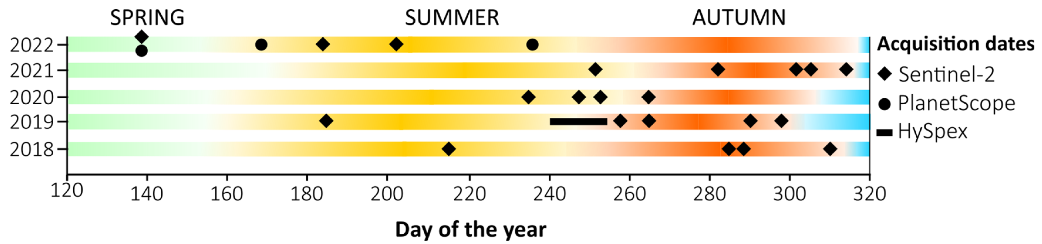
The high-mountain areas of central Europe are characterized by dynamic weather due to the influence of the Atlantic and continental climates, which result in the lifting of warm air masses, where condensation and cloudiness occur, which cause windbreaks, changing the age and species structure of forest stands. Therefore, obtaining scenes representing various stages of vegetation development is challenging. Hence, we need to analyze multiseasonal series to help capture phenology. Additionally, because the growing season in the mountains is short and the spectral properties of vegetation quickly change, we used multitemporal Sentinel-2 compositions. As the reference data, we collected field-verified polygons, representing pixels of all analyzed species located in different topographic patterns with different elevations, slopes, and aspects. In different topographic locations, the same species has different spectral signatures as a result of the influences of water vapor, insolation, wind, and temperature. These factors play key roles in leaf drying, which forces the plant to adopt protective mechanisms that affect spectral responses. Ecosystem heterogeneity (plant communities, rocks, dry trunks, branches, and other objects) generates mixels through the effect of the neighborhood, which influences the spectral responses registered by airborne and satellite sensors and thereby the classification results [30]. The HySpex reference data have a spatial resolution of 2 m and a spectral resolution of 430 bands, which seems to be an advantage; however, the pixel size is comparable to the size of a tree crown. Additionally, the availability of long-term Sentinel-2 data substantially improves the ability to identify tree stands, especially when individual species implement different growth and development strategies during the vegetative period. Capturing spectral variation during the phenological season can remarkably increase the accuracy of the classification results and indicates which data selection scenarios allow us to obtain satisfactory results.

The use of data and open-source software allows for the constant monitoring of the environment without incurring burdensome costs, which is especially valuable for NGOs or nature conservation areas that have teams of several specialists dealing with nature monitoring, as well as well-qualified foresters who can verify the observed changes on an ongoing basis. Additionally, Sentinel-2 imaging covers the entire area at once, which reduces radiometric differences and ensures spectral coherence; the relatively short revisit time allows for the elimination of gaps created by single clouds. In comparison, airborne campaign planning is much more demanding due to size of the study area, elevation differences, and weather dynamics. As such, airborne campaigns often last for several days and include the acquisition of various fragments in different weather conditions, which may change the properties of the spectral analysis of the analyzed objects and thus increase the imaging cost. Satellite data allow the acquisition of objective and repeatable data for long-term environmental monitoring [31], and the obtained results can be reliably applied to other mountain areas, which allows the identification of changes in alpine ecosystems located in different parts and zones in Europe and around the world.

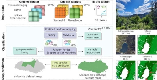
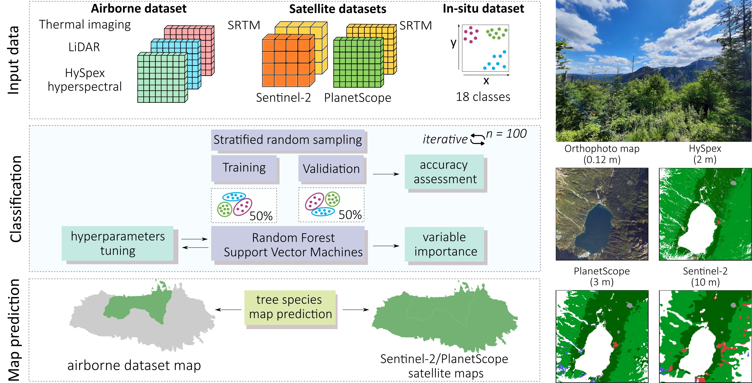
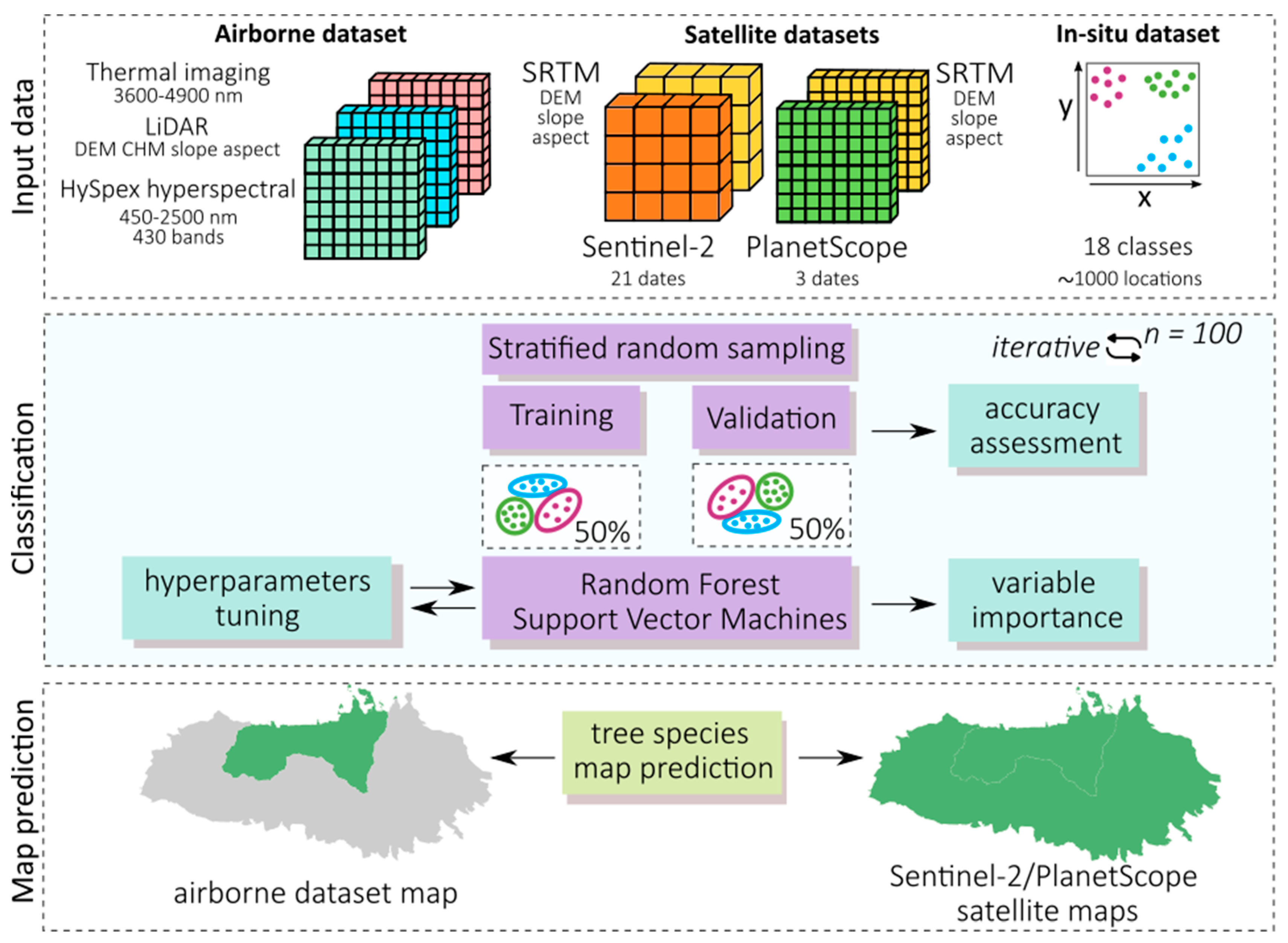
Our aim in this study was to assess the free Sentinel-2 data with commercial PlanetScope and airborne HySpex hyperspectral data for mapping the dominant woody species of the Tatra Mountains, which is a challenging research objects due to the substantial elevation differences in the area, as well as its various aspects and slopes, which create a mosaic of spectral features. Therefore, one of our objectives in this study was to assess the impact of topographic feature derivatives on the accuracy of the identification of coniferous and deciduous tree species. Because the greening-up period, maturity, senescence, and dormancy of individual species depend on elevation, slope, and aspect, the analyses for the same species depend on the topography. The Tatra forest ecosystem is characterized by high heterogeneity of species, which form different-sized groups of individual trees. Additionally, the variability in age, dry tree trunks, and branches causes a large mix of the signals recorded in individual pixels, which complicates the identification of the dominant objects; this directly affects the ability to identify individual species. Due to the occurrence of individual species in hard-to-reach places, e.g., Swiss stone pine (Pinus cembra, where single individuals are identified on mountain tops), species appear in all topographically analyzed patterns (elevation, slope, and aspect); therefore, an important issue in this study was testing different sizes of balanced samples to assess their impact on the classification result. For this reason, we applied an iterative classification method: we performed each classification iteration based on randomized selected patterns, which we independently selected for each iteration, and we repeated the whole process 100 times. This allowed us to test the spectral variability in the analyzed patterns and the impact of the number of training pixels on the obtained results. Therefore, the classification process was based on a large number of field-verified polygons to capture the diversity of forms of individual species occurring both on homogeneous plots and in the areas where several species coexisted. As classifiers, we used the R-based open-source programming libraries for the SVM and RF algorithms.

The main study question was to assess the classification accuracy of the dominant woody species in protected mountain areas based on airborne hyperspectral HySpex data as well as commercial high-resolution PlanetScope and open-access Sentinel-2 satellite data. We conducted the analyses to assess if investing in commercial imaging is profitable and if multitemporal Sentinel-2 images can be used to obtain sufficiently accurate spectral characteristics during the vegetative period to enable the successful identification of woody species of natural forests, which are much more heterogeneous in terms of tree composition and age compared with managed forests.

2. Materials and Methods

2.1. Study Area

The study area covered the core and buffer zone of the UNESCO Tatra Transboundary Biosphere Reserve, occupying nearly 1000 km² area, which is formed by the Polish Tatra National Park (TPN) and Slovakian Tatranský národný Park (TANAP), with area shares of 22% and 78%, respectively (Figure 1). The Tatras are the highest mountain range in the Carpathians, with some peaks exceeding 1500 m. The High Tatras are characterized by alpine ecosystems. Erosion-resistant granodiorite is the dominant substrate of the High Tatras, which are located in the eastern part of the Tatras; the southern part of the western Tatras consists of the metamorphic rocks; the northern part is characterized by less resistant formations: carbonate rocks [32]. The climate of the Tatras is highly variable, depending on the altitude. The average annual temperature varies between 4 and −3 °C, whereas mean temperature in the coldest and warmest month varies from −6 to −11 °C and 4 to 15 °C, respectively [33]. The number of days with snow cover ranges from 120 to 220 days, and annual precipitation varies from 1000 to 1700 mm, increasing with altitude [33]. The annual mean total cloud cover for 1991–2020 was 68%, which was calculated based on ERA5 (European Centre for Medium-Range Weather Forecasts (ECMWF) Reanalysis 5th Generation) climate reanalysis data [34]. Strong foehn winds cause serious forest stand damage and windthrow, which accelerate the changes in vegetation cover [35]. The long snow cover duration, high precipitation, large total cloud cover [36], and short growing season create challenges for obtaining remote sensing data of vegetation in this area.

The forest stands of the Tatra Mountains are mainly composed of coniferous species [37] and a smaller share of deciduous species (Figure 2), characterized by altitudinal zonation. Large elevation and topography changes and the lack of roads [38] hinder research in the Tatras. The Tatras are a protected area, where the management is different from that for commercial forests, which influences the proportion of particular species, amount of dead wood, as well as the compactness and forest gaps caused by numerous disturbances. These mountains provide a habitat for three large carnivoran species (brown bear, grey wolf, and Eurasian lynx) that are protected in this area. Currently, large changes are occurring in the forest stands [39] caused by bark beetles, windthrow, climate change, and air pollution. Spruce monocultures that were artificially planted have declined and formed snags with deciduous species growing under them [40].

2.2. Satellite and Airborne Data

For vegetation classification, we used three datasets: open-access satellite Sentinel-2, commercial satellite PlanetScope, and airborne HySpex data. The Sentinel-2 surface reflectance processing level-2A products were obtained from ESA’s Copernicus Open Access Hub service. We acquired 21 images for the years 2018–2022, which we chose because no substantial changes in the shares of vegetation types occurred in this period. Although images for the study area are acquired by Sentinel-2 satellites every 2–3 days, due to the high cloud cover typical of mountainous areas, an average of four cloudless scenes per year were retrieved (Figure 3). The study area was covered by two tiles (34UCV and 34UDV) located in the same orbits (track 79 or 36).

We used the twelve Sentinel-2 channels, which we processed in ESA SNAP 9.0 software, with resampling performed using the nearest neighbor method for 10 m pixel sizes. We mosaicked images from the two tiles based on the same date as well as the orbit; next, we stacked all scenes into a data cube of multitemporal composition. The use of multitemporal compositions is especially relevant in mountainous areas where shadows are imposed on the slopes by the high peaks. On different acquisition dates, images with different solar elevation and azimuth angles are collected, so the shadows on the slopes can be eliminated.

For elevation data, we used the 1 arc-second global product (~30 m pixel size) based on Shuttle Radar Topography Mission (SRTM) obtained from the USGS Earth Explorer service. The area included two tiles (N49E019 and N49E020), which we mosaicked and then resampled to 10 m resolution and matched with the Sentinel-2 pixel grid. We calculated topographic derivatives, such as slope and aspect metrics, in degree values from the SRTM digital elevation model (DEM) using the R language raster package [41]. The data were then standardized to a unified coordinate system (EPSG: 32634) and combined with Sentinel-2 optical imagery.

Additionally, for the whole area of Tatra Mountains, we used PlanetScope data from three dates of different vegetation periods (19 May 2022, 19 June 2022, and 26 August 2022) [42]. The imagery was derived from the third generation of Super Dove satellites with an installed PSB.SD instrument (3 m pixel size, 8 spectral bands, and 16-bit radiometric resolution), which have a spectrum interoperable with those of the Sentinel-2 bands in 6 channels [43]. We used the analytic OrthoScene product (level 3B), which was orthorectified, geometrically corrected, and radiometrically calibrated to surface reflectance [44], for the study. Satellite imagery was verified using the QA band for the detection of any potential distortions. Next, we mosaicked and stacked the images to create a single multitemporal composition using the GDAL [45] open-source library, which we merged with SRTM topographic features bands that we had resampled to 3 m (Figure 4).

For the Polish part of the Tatra Mountains, airborne data were acquired in 2019 based on a multisensor platform mounted onboard a Cessna 402B aircraft owned and operated by the MGGP Aero company, which acquired and processed the airborne data. A HySpex VS-720 hyperspectral camera (Norsk Elektro Optikk, Norway) was used (configuration: 1x VNIR-1800 and 2x HySpex SWIR-384 cameras) with two-meter pixels registered in 430 bands in the spectrum range of 400–2500 nm, with a full width at half maximum of 3.8–6.5 nm and a field of view (FOV) of 34°. The radiometric resolution was 16 bits with 30% coverage. Airborne laser scanning (ALS) data were acquired with a Riegl VQ-780I sensor (by Riegl GmbH), whose spectral range of the full-waveform beam type was 1064 nm, FOV was 50°, and scanning density was 8 points/m². The LiDAR data were then processed using LASTools software [46] and the R lidR package [47], generating topographic derivatives including digital elevation model, canopy height model, and slope and aspect maps. Thermal data were acquired with an ImageIR 9400 camera (by InfraTec GmbH) registering in the middle-wave infrared spectrum range (3600–4900 nm), with a spatial resolution of 1 m and an average emissivity parameter set to 0.95. Finally, we resampled all data, which we matched to the HySpex pixel resolution, gridded, and compacted into a single data set. In addition, we used a high-resolution orthophoto map data in RGB and CIR (pixel size: 0.12 m) to validate the polygons acquired in the field, but the images were not used for classification.

2.3. Reference Data, Classification, and Accuracy Assessment

We focused on the main woody species present in the Tatra Mountains (

Table 1. Dominant woody species and background classes collected in situ for training and testing.

Class Name (Common Name)	Type	No. of Polygons	No. of Pixels
			HySpex	PlanetScope	Sentinel-2
Sycamore (Acer pseudoplatanus)	broadleaf	104	2042	1298	209
Grey alder (Alnus incana)	broadleaf	25	387	342	168
European beech (Fagus sylvatica)	broadleaf	108	5673	4343	482
European ash (Fraxinus excelsior)	broadleaf	15	47	43	17
Willow (Salix spp.)	broadleaf	29	659	516	115
Rowan (Sorbus spp.)	broadleaf	42	2078	1376	114
Silver fir (Abies alba)	conifer	46	795	757	122
Larch (Larix spp.)	conifer	47	438	387	177
Norway spruce (Picea abies)	conifer	157	24,102	19,422	10,251
Swiss stone pine (Pinus cembra)	conifer	25	114	100	13
Dwarf mountain pine (Pinus mugo)	conifer	76	28,092	16,501	5236
Scots pine (Pinus sylvestris)	conifer	14	71	67	101
Snags	conifer	30	1009	981	893
Alpine grasslands	background	87	3264	2919	1363
Low shrubs		73	4550	4452	4551
Other nonforest		17	6534	4356	633
Rocks and artificial surfaces		59	4324	4228	3754
Water		14	82,188	74716	9519
Total		968	166,367	136,804	37,718

) [48]. Other species, such as sparse birches (Betula pubescens, B. obscura, and B. pendula), lime trees (Tilia cordata and T. platyphyllos), black pine (Pinus nigra), and others, are found here but they account for only a small proportion of the admixture in the survey area, so are indistinguishable with satellite methods due to the size of the crowns in the Sentinel-2 pixel. As such, they were excluded from the study. Three field campaigns were conducted (9–13 September 2021; 29 April–3 May 2022; 15–25 July 2022) on the Polish side (TPN), because airborne remote sensing data set were provided only for this area. The result of the field study was the verification of permanent monitoring plots in the park as well as the identification of additional, large, homogeneous areas, which allowed us to identify 968 patterns of 18 classes, including 13 woody species on 718 polygons (7 coniferous and 6 broadleaf) and 5 other land cover classes (aggregated into a single background class; Table 1). Within the coniferous species, the snags class was also included because of being mainly composed of wind throws and dead Norway spruce. For classification, we decided to use additional background classes that represented the rest of the land cover classes present in the area, rather than masking no-forest areas using, e.g., a canopy height model. This was driven by the need to compare two separate data sets where the mask of the more spatially accurate HySpex data (pixel size: 2 m) did not overlap with the Sentinel-2 mask (pixel size: 10 m) because of offsets and pixel spatial resolution, which was particularly important for objective comparisons between the two data sets. Additionally, low-growing dwarf pine and young trees created complications when applying the mask as these would not be included. Therefore, introducing background classes was more efficient, which is a widely used approach [49,50,51,52]. Using this method, we could also verify that the tree classes did not mix with other classes, e.g., low shrubs, which was especially relevant due to the discontinuity and mosaic characteristics of the vegetation in the study area.

For the three classes of tree species, aggregation was conducted by identifying these as several species of larch (Larix decidua, Larix kaempferi, and Larix × eurolepis), willows (Salix silesiaca, Salix aurita, Salix caprea, and others), and rowans (Sorbus aucuparia and Sorbus intermedia), which, individually, accounted for small proportions of the admixtures, so were difficult to detect or they were hybrids. We attempted to ensure that the field-collected data were equally distributed over the entire park area and at different heights, slopes, and exposures to avoid autocorrelation and provide high-quality spectral signatures [53] that most accurately represented the characteristics of the Tatra forest stands for the classification algorithms (Figure 5). Then, we verified the locations of the woody species obtained in the field on a high-resolution orthophoto in RGB and CIR (0.12 m) and on the canopy height model.

Because of the difficulty of conducting surveys in mountainous areas, we also tested the effect of pixel size on the classification accuracy to obtain information on the optimal number of pixels to achieve a given classification accuracy [54]. In addition, balanced sets have a favorable effect on the classification of rare plant species, where obtaining a sufficient number of patterns is impossible, so that imbalanced sets may be unrepresented in the classifier and then poorly classified [55]. Considering the altitudinal zonation characteristics of mountainous areas, we investigated the influence of topographic variables extracted from SRTM and LiDAR on classification accuracy. For the presentation and comparison of results, we mainly relied on the F1-score (F1-score = 2 × (𝑃𝐴 × 𝑈𝐴)/(𝑃𝐴 + 𝑈𝐴), where PA is producer accuracy, and UA is user accuracy) due to its higher objectivity, and the combination of user and producer accuracy. Concerns have been raised in the literature about measures such as kappa [56] and overall accuracy [57], which may influence the outcome and impede the comparability of results between studies. For classification, we used two algorithms: random forest [58] and support vector machine [59]. We tuned the hyperparameters of the algorithms using the grid search method for all combinations of parameters, followed by ten-fold cross-validation. For the SVM with the radial kernel function (RBF), we tested the cost and gamma parameters based on the mean F1-score values for all classes; for random forest, we tuned the ntree and mtry parameters based on the out-of-bag (OBB) error (

Table 2. Selected input hyperparameters of algorithms (random forest and support vector machine) using grid search method.

Sensor	Number of	SVM	SVM	RF	RF
	Bands	Cost	Gamma	ntree	mtry
HySpex	430	100	0.1	500	240
Sentinel-2	252	10	0.01	500	120
PlanetScope	24	100	0.01	500	10

).

Subsequently, we assessed the iterative accuracy 100 times on the optimized classifiers, where, for each iteration, the training and test sets were randomly split by polygons in 50:50 ratio using stratified random sampling to ensure the test and validation set independence [60]. Then, the classifier was trained, and the achieved classification accuracy was verified. We also checked the effects of the variable importance of the individual Sentinel-2 channels and the acquisition dates of the images on classification accuracy during classification. We used the classifiers with the highest mean F1-scores to predict the output images, which we then filtered with a 3 × 3 median filter. Classifications on HySpex data were performed for the Polish Tatra area, and classifications with Sentinel-2 and PlanetScope imagery were performed for the entire Tatra area (Poland and Slovakia).

3. Results

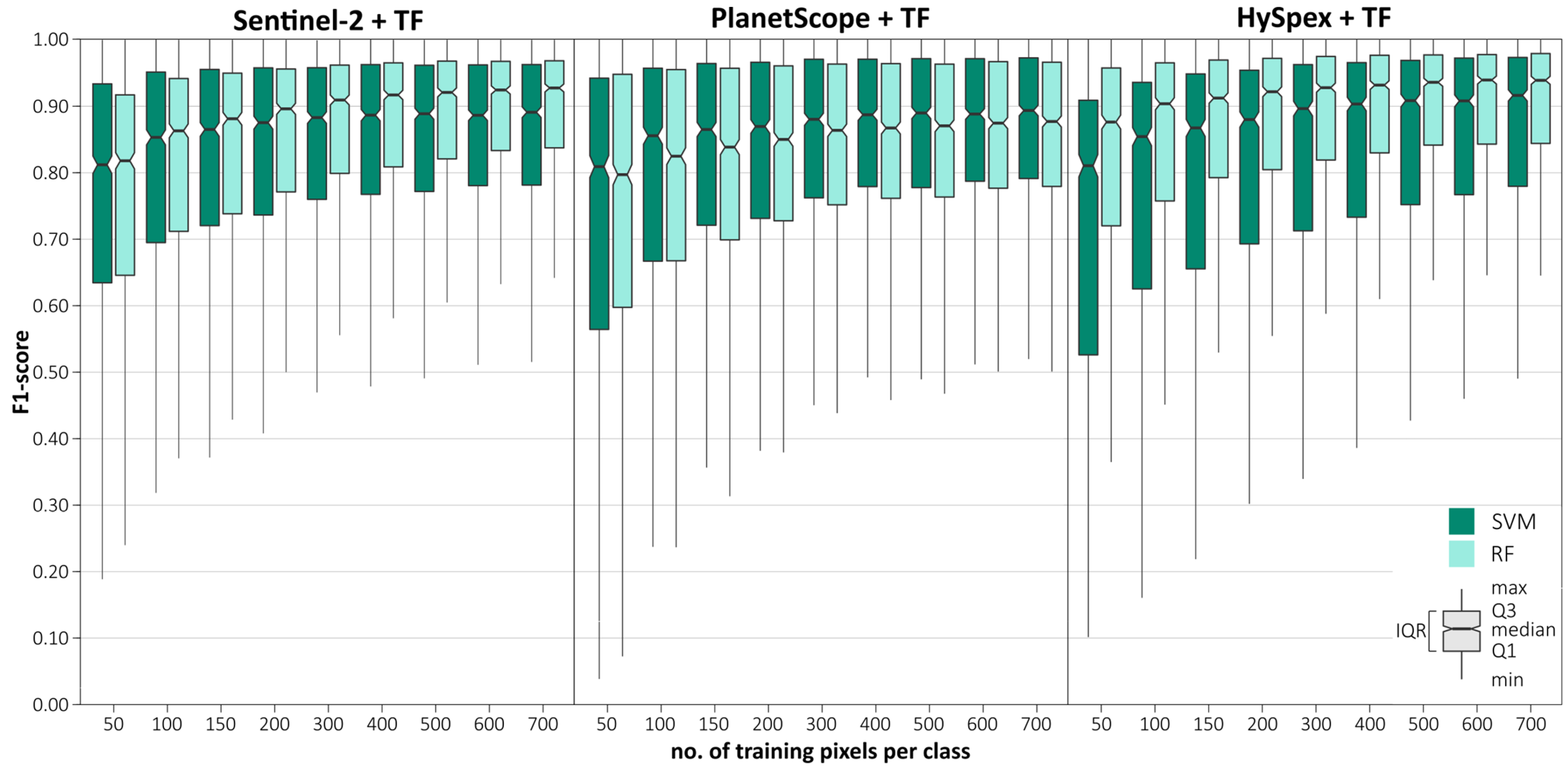
In the first stage, we aimed to determine the effect of the number of pixels on classification accuracy (from 50 to 700 pixels; Figure 6). We obtained the highest median F1-score for the maximum number of pixels used (700): Sentinel-2 (0.93 RF; 0.89 SVM), PlanetScope (0.89 RF; 0.87 SVM), and HySpex (0.95 RF; 0.92 SVM). The results for the HySpex data were characterized by a high interquartile range (0.15–0.38), with a particularly large difference between the SVM and RF algorithms (by 0.06–0.15), followed by the PlanetScope data (0.17–0.31). We observed the narrowest range for the Sentinel-2 data (0.11–0.23); however, in this case, we found no difference between RF and SVM (0.01–0.05). As the number of pixels increased, the interquartile ranges of the results tended to decrease, by 0.03 per 100 pixels on average. The range increased by an average of 0.02 for every 100 pixels, with the largest increase observed between 50 and 200 pixels (by 0.04–0.09), whereas the difference between 50 and 700 pixels was 0.09–0.13. The results stabilized between 500 and 700 pixels and then changed little (0.01–0.02). Therefore, we considered the value of 700 pixels as optimal, which we used for further classification and analysis.

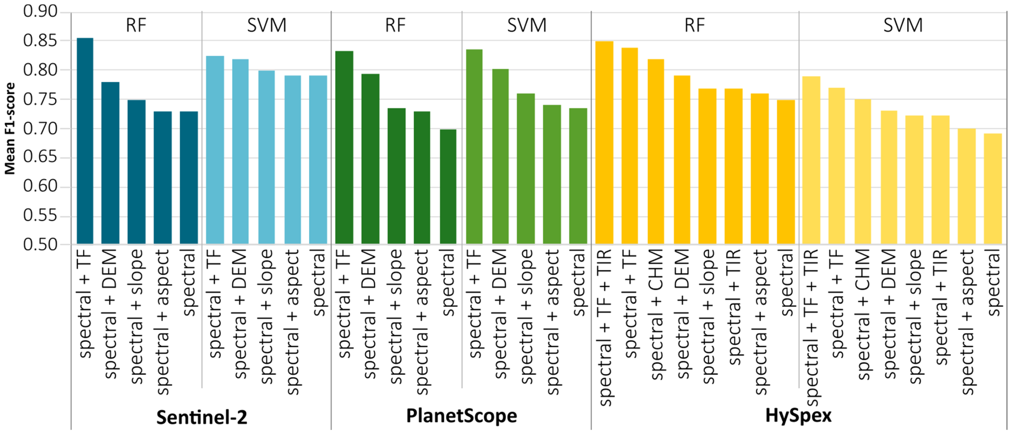
The average F1-score for the topographic features data (Figure 7) oscillated around 0.77–0.86: Sentinel-2 (0.86 RF; 0.82 SVM), PlanetScope (0.83 RF; 0.84 SVM), and HySpex (0.84 RF; 0.77 SVM). The random forest algorithm performed better on the Sentinel-2 (by 0.04) and HySpex (by 0.07) data, whereas the SVM was more accurate on PlanetScope imagery (by 0.01). As shown by the results, using only spectral data, without any additional data, produced less accurate performance of 0.10 (range: 0.69–0.77) on average. Analyzing the influence of individual topographic variables (Figure 7), the most accurate results were achieved by digital elevation model, which improved the results (by 0.04–0.10) in relation to the spectral data, followed by slope (by 0.01–0.03). Aspect least affected the result, only slightly increasing the classification accuracy (0.01–0.02), because the occurrence of forest stands in this area is only slightly influenced by direction. As such, aspect is more important in nonforest communities (shaded areas with accumulated snow affecting the type of vegetation). For hyperspectral data, we used airborne laser scanning derivatives, for which additional input was provided by the canopy height model, which increased the accuracy by 0.04, and thermal data, by 0.03. The combination of all topographic variables provided the best results, which increased the accuracy on average by 0.10 compared with those using spectral data. We found the smallest differences for Sentinel-2 imaging with the SVM algorithm, where the impact was small (by 0.05); we found the biggest differences for PlanetScope data with the RF classifier (by 0.14).

The next step was checking the relevance of the individual dates and channels of the PlanetScope (

Table 3. Relationship of variable importance (mean decrease in accuracy) between PlanetScope bands and acquisition dates (values for topographic features; DEM: 94.4; slope: 30.7; aspect: 9.3). The importance of the bands was confirmed by the intensity of the green color.

Date	B1	B2	B3	B4	B5	B6	B7	B8	Mean
2022-05-19	24.4	28.8	35.7	28.1	19.5	41.1	29.9	72.8	35.1
2022-06-19	16.5	13.8	24.9	38.2	22.8	28.4	36.8	45.0	28.3
2022-08-26	20.1	27.1	22.7	25.3	28.0	18.2	19.3	20.5	22.7
Mean:	20.4	23.2	27.8	30.5	23.5	29.2	28.7	46.1
Score	8	7	5	2	6	3	4	1
Central wavelength (nm)	443	490	531	565	610	665	705	865
Interoperable with Sentinel-2	S-2 B1	S-2 B2	No equivalent	S-2 B3	No equivalent	S-2 B4	S-2 B5	S-2 B8A

) and Sentinel-2 (

Table 4. Relationship of variable importance (mean decrease in accuracy) between Sentinel-2 bands and acquisition dates (values for topographic features; DEM: 54.8; slope: 12.7; aspect: 5.4). The importance of the bands was confirmed by the intensity of the green color.

Date	B1	B2	B3	B4	B5	B6	B7	B8	B8A	B9	B11	B12	Mean
2018-08-03	5.8	3.5	3.7	6.1	5.6	4.4	4.6	5.4	5.5	6.3	5.0	5.3	5.1
2018-10-12	4.8	3.4	2.5	3.4	3.4	3.4	3.2	4.4	4.0	2.8	4.2	4.0	3.6
2018-10-15	4.6	3.8	3.5	1.7	6.9	3.6	11.0	4.9	3.5	1.3	4.3	4.1	4.4
2018-11-06	5.2	3.5	4.3	3.8	3.5	4.8	9.6	2.9	3.3	2.8	3.1	4.0	4.2
2019-07-04	5.7	9.9	4.7	9.5	9.6	7.5	5.2	5.4	6.6	9.6	4.6	3.6	6.8
2019-09-15	5.2	14.4	5.1	3.9	2.4	4.9	3.8	6.9	9.5	8.5	5.4	4.8	6.2
2019-09-22	4.9	6.2	8.3	6.0	4.6	4.1	4.5	3.9	7.8	4.3	3.7	6.4	5.4
2019-10-17	4.8	2.9	3.5	3.8	4.5	9.1	4.6	2.4	3.2	3.6	3.0	3.9	4.1
2019-10-25	5.6	4.3	3.8	3.0	9.5	4.8	12.0	3.8	3.6	2.9	3.8	3.7	5.1
2020-08-22	5.5	2.5	4.1	5.9	7.7	4.3	4.7	7.7	4.5	6.6	5.6	4.0	5.2
2020-09-04	5.2	8.5	6.3	4.1	4.1	3.4	3.2	5.9	7.2	6.5	6.2	4.6	5.4
2020-09-09	4.6	3.6	5.8	3.3	4.2	2.3	4.0	5.3	3.5	4.1	5.7	3.3	4.1
2020-09-21	6.7	2.0	3.3	1.8	2.9	2.5	2.1	3.2	3.4	4.1	2.9	3.5	3.2
2021-09-09	4.2	7.4	3.4	4.2	4.2	4.2	4.9	7.8	5.0	4.1	5.0	4.0	4.9
2021-10-09	8.1	3.7	3.7	2.9	6.2	4.5	3.9	2.3	2.0	1.7	2.7	4.0	3.8
2021-10-29	5.6	6.4	5.3	3.4	5.8	6.3	8.1	4.2	3.7	3.2	3.7	3.6	5.0
2021-10-31	3.5	5.5	4.8	3.5	7.0	6.9	6.9	2.7	2.1	4.1	4.0	2.5	4.4
2021-11-10	5.5	6.1	5.2	5.0	4.0	5.8	3.8	3.0	1.7	3.9	2.3	4.8	4.2
2022-05-19	4.2	6.0	5.1	7.8	10.4	17.3	7.2	10.9	9.3	10.4	10.4	4.8	8.7
2022-07-03	3.4	8.3	5.9	8.1	11.4	14.3	5.4	9.5	9.0	10.1	6.0	3.6	7.9
2022-07-21	5.5	5.1	4.2	9.4	9.2	15.1	4.9	6.9	4.7	9.2	6.0	2.3	6.9
Average:	5.2	5.6	4.6	4.8	6.1	6.4	5.6	5.2	4.9	5.3	4.6	4.0
Score	7	4	10	9	2	1	3	6	8	5	11	12
Central wavelength (nm)	443	490	560	665	705	740	783	842	865	940	1610	2190
Spatial resolution (m)	60	10	10	10	20	20	20	10	20	60	20	20

) multitemporal composites. Comparing the influence of individual bands on the classification result using the mean decrease in accuracy (MDA) value, we observed the following: the most important period for the identification of forest stands is spring (month of May); this is when fully formed leaves of conifers can be observed. However, depending on the species, young leaves, needles, and shoots develop at difference paces; their color, shape, and size depend on the species as well. Another important observation was the usefulness of the red-edge bands, in the case of PlanetScope: the red-edge (B8), green (B3), red (B7; Table 3), and for the Sentinel-2 the most informative were the 20 m channels B6, B5, B7, 10 m B2, and 60 m B9 (SWIR; Table 4). This was expected because, due to plant pigments, the visible and red-edge range as well the cell structures in NIR play key roles in vegetation analyses. Notably, the red-edge range, which provides information about the condition of vegetation, played a key role in both cases.

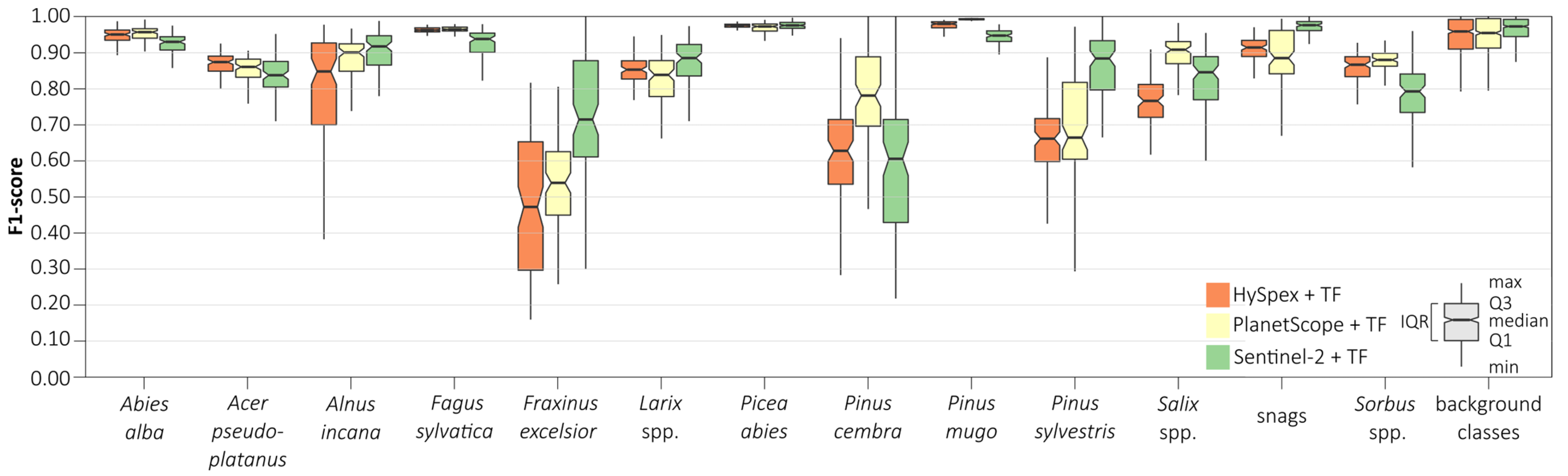
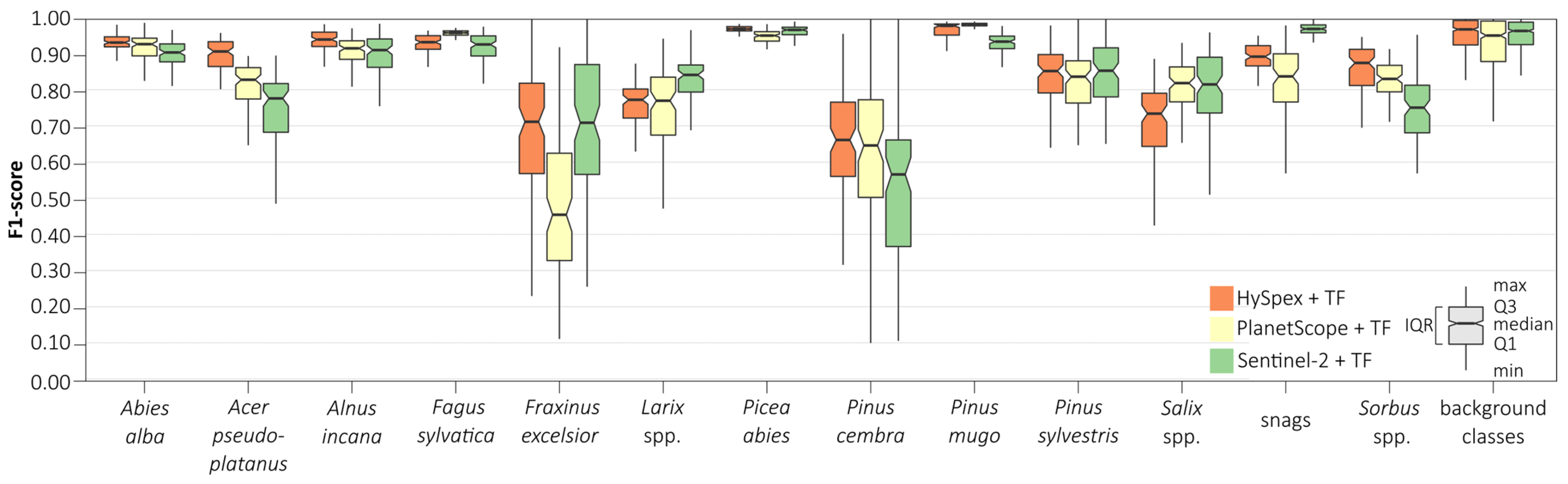
We conducted an iterative assessment of classification accuracy for each class depending on the dataset used based on the random forest (Figure 8) and support vector machines (Figure 9) classifiers. We obtained the highest median scores (above 0.90) for all remote sensing sets for the following classes: silver fir (Abies alba; 0.91–0.95), European beech (Fagus sylvatica; 0.92–0.96), Norway spruce (Picea abies; 0.97–0.98), dwarf mountain pine (Pinus mugo; 0.95–0.99), and grey alder (Alnus incana; 0.87–0.92). We obtained the lowest ones for European ash (Fraxinus excelsior; 0.44–0.72), Swiss stone pine (Pinus cembra; 0.58–0.78), and Scots pine (Pinus sylvestris; 0.67–0.85), which were also characterized by wide median differences (0.02–0.25) among the results obtained between the different remote sensing datasets. The widest interquartile range (IQR) was obtained for rare classes: European ash (Fraxinus excelsior; 0.10–0.32), Swiss stone pine (Pinus cembra; 0.20–0.27), and Scots pine (Pinus sylvestris; 0.12–0.38); we obtained the narrowest IQR for silver fir (Abies alba; 0.03–0.05), sycamore (Acer pseudoplatanus; 0.04–0.08), European beech (Fagus sylvatica; 0.01–0.05), Norway spruce (Picea abies; 0.01–0.02), and dwarf mountain pine (Pinus mugo; 0.01–0.02). We observed similar patterns for the SVM classifier, but these interquartile ranges for most classes were notably wider (by 0.01–0.07). Analyzing various classification scenarios, we found that random forest produced the most accurate classification results on Sentinel-2 and PlanetScope images, whereas support vector machine was more appropriate for HySpex data.

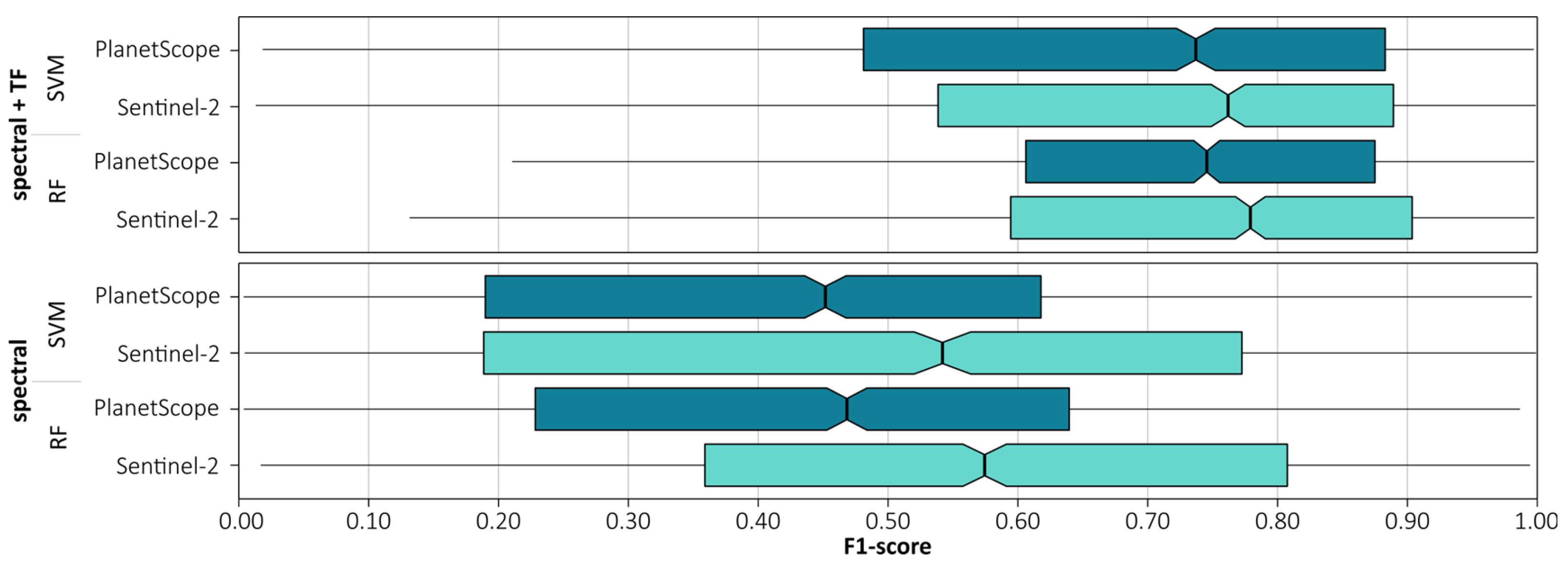
We also compared the classifications between PlanetScope and Sentinel-2 for the same acquisition date (19 May 2022) and time (approximately 9:00 UTC), allowing for the same conditions of solar irradiance and incidence angle (Figure 10). Sentinel-2 spectral data outperformed PlanetScope data for both the random forest (0.58 vs. 0.47 F1-score) and support vector machine (0.53 vs. 0.45 F1-score) classifier. The differences between the classifiers substantially decreased when topographic derivatives were included, by an average of 0.23 points. However, the results obtained using Sentinel-2 data still scored higher (RF: 0.78, SVM: 0.76) than those obtained using PlanetScope data (RF: 0.74, SVM: 0.73), indicating the importance of including topographic product data in mountain vegetation analyses. Even with a single scene, high accuracy can be achieved.

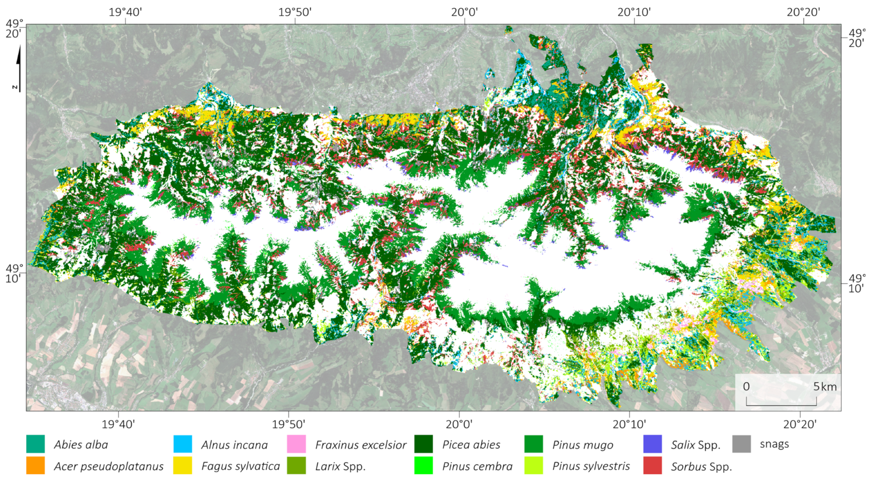
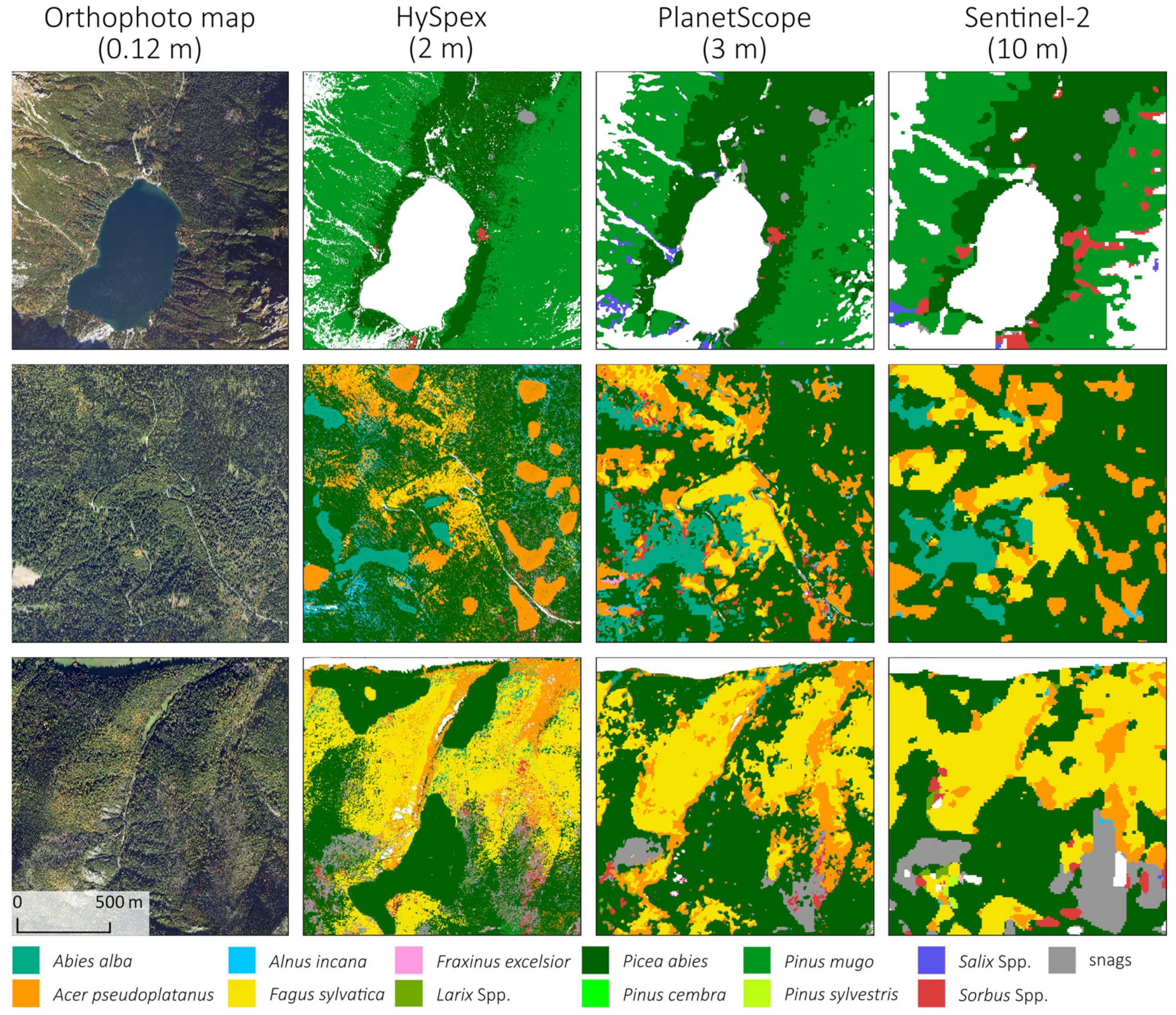
Based on the best classification results according to the mean F1-score for tree species classes, we classified the tree species in the Tatra Sentinel-2 area (Figure 11;

Table 5. Error matrix of obtained Sentinel-2, with topographic features and Random Forest classification results presented on Figure 11. S.f.—silver fir (Abies alba); Syc.—sycamore (Acer pseudoplatanus); G.a.—grey alder (Alnus incana); E.b.—European beech (Fagus sylvatica); E.a.—European ash (Fraxinus excelsior); Lar.—larch (Larix spp.); N.s.—Norway spruce (Picea abies); S.s.p.—Swiss stone pine (Pinus cembra); D.m.p.—dwarf mountain pine (Pinus mugo); S.p.—Scots pine (Pinus sylvestris); Wil.—willow (Salix spp.); Row.—rowan (Sorbus spp.); AG—alpine grasslands; LO—low shrubs; ON—other nonforest; RS—rocks and artificial surfaces; WA—water; UA—user accuracy; F1—F1-score; PA—producer accuracy.

	S.f.	Syc.	G.a.	E.b.	E.a.	Lar.	N.s.	S.s.p.	D.m.p.	S.p.	Wil.	Snags	Row.	AG	LO	ON	RS	WA	Σ	UA	F1
S.f.	45	1	0	0	0	1	8	0	0	0	0	0	0	0	0	0	0	0	55	0.82	0.81
Syc.	0	70	0	8	0	0	1	0	0	0	1	0	0	0	0	0	0	0	80	0.88	0.86
G.a.	2	1	103	1	0	6	13	0	0	0	0	0	0	0	0	0	0	0	126	0.82	0.90
E.b.	3	10	0	390	0	6	0	0	0	0	0	0	1	0	0	0	0	0	410	0.95	0.95
E.a.	0	0	0	0	8	0	0	0	0	0	0	0	0	0	0	0	0	0	8	1.00	1.00
Lar.	0	0	0	1	0	94	0	0	0	0	0	0	0	0	0	0	0	0	95	0.99	0.87
N.s.	6	0	0	2	0	15	4909	0	1	1	2	24	11	0	27	0	36	2	5036	0.97	0.98
S.s.p.	0	0	0	0	0	0	0	6	0	0	0	0	0	0	0	0	0	0	6	1.00	0.86
D.m.p.	0	0	0	0	0	0	0	0	2744	0	0	0	2	1	153	0	4	0	2904	0.94	0.93
S.p.	0	0	0	0	0	0	0	0	0	51	0	0	0	0	18	0	2	0	71	0.72	0.83
Wil.	0	0	0	0	0	0	0	0	15	0	85	0	0	0	29	0	0	0	129	0.66	0.74
Snags	0	0	0	0	0	0	0	0	0	0	0	582	0	0	4	0	24	0	610	0.95	0.93
Row.	0	0	0	2	0	0	1	0	188	0	8	33	72	0	26	0	0	0	330	0.22	0.34
AG	0	0	0	0	0	0	0	0	0	0	0	0	0	755	39	0	34	0	828	0.91	0.93
LO	0	0	0	3	0	0	0	2	1	0	4	0	7	24	2779	0	0	0	2820	0.99	0.94
ON	0	0	0	3	0	0	0	0	0	0	0	0	0	0	0	249	0	0	252	0.99	0.99
RS	0	0	0	0	0	0	0	0	30	0	0	0	0	10	5	0	882	0	927	0.95	0.92
WA	0	0	0	0	0	0	32	0	0	0	0	0	0	0	0	0	0	4635	4667	0.99	1.00
Σ	56	82	103	410	8	122	4964	8	2979	52	100	639	93	790	3080	249	982	4637
PA	0.80	0.85	1.00	0.95	1.00	0.77	0.99	0.75	0.92	0.98	0.85	0.91	0.77	0.96	0.90	1.00	0.90	1.00

), as well as for PlanetScope and HySpex imagery, the locations of which were compared with each other (Figure 12). For this purpose, we selected three areas (dimensions: 1.5 km × 1.5 km = 225 ha) at different elevations and with different stand characteristics to reflect the diversity of the Tatra stands (deciduous, coniferous, and forests undergoing large-scale transformations) and to check the repeatability of the results. The obtained maps and error matrices (Table 5 and Appendix A) showed high convergence and a pattern of tree stand occurrence, with differences mainly due to the spatial resolution of the data (2, 3, and 10 m), the angle of sunlight incidence, and the effect of shadows. The maps were compared with a very-high-resolution orthophoto map (pixel size: 0.12 m).

4. Discussion

The results of our analyses confirmed the high potential of remote-sensing-based methods for the identification of forest species in protected areas. Despite the heterogeneity of the environment and topographic features, we successfully identified all dominant woody species of the Tatras, and the results should be considered satisfactory: for 10 out of 13 species, we obtained an average F1-score above 0.80, 6 of which were above 0.90. The accuracy of coniferous species identification was slightly higher on average (F1: 0.87) than for broadleaf species (F1: 0.84). Even these rarer species were well-identified on the Sentinel-2, PlanetScope, and HySpex images, allowing their successful identification on larger polygons in some areas of the TPN. However, in general, as they did not create compact and homogeneous surfaces, most of the identified patterns had error (IQR values were high) resulting from the share of other species, which created mixed tree crowns. Comparing our outcomes with those of other authors (Table 6), our results obtained from HySpex images are a few percentage points higher than those of Shi et al. [61], who used the same algorithm (RF). Our results are similar to those of Raczko et al. [62], who used ANN and 280 spectral channels from APEX aerial imaging for the Karkonosze Mountains (mountain forests on the border of Poland and the Czech Republic). The proposed method of using multitemporal Sentinel-2 scenes (252-band data cube from 21 scenes representing different vegetation periods), allowed us to identify the studied species with higher accuracy than if we had used deep neural classifiers (CNN [26] and XGB [63]). Xi et al. [64], comparing different algorithms, confirmed the dominance of RF over three other types of deep neural network (Conv1D, AlexNet, and LSTM) for a few species, which we identified (Table 6), as well as for Manchurian ash classification. Additionally, RF produced results similar to those of Conv1D, AlexNet, LSTM, and SVM for Dahurian larch and white birch. RF scored worse than the best Conv1D classifier by approximately 6–8 percentage points in identifying Amur linden, Korean pine, and aspen [64].

Waser et al. [65], in mapping the dominant leaf type based on Sentinel-1/-2 data, found that UNet convolutional neural networks and RF obtained similar results; in some cases, UNet obtained worse results, depending on stand characteristics, type, and heterogeneity. Additionally, mapping a relatively low number of species (aspen, birch, pine, and spruce) on Sentinel-2 imagery, despite testing different types of CNN architectures, resulted in moderate F1-score of 0.68–0.76 using UNet with a ResNet encoder [66] or 0.42–0.85 for feature pyramid network (FPN) with EfficientNet infrastructure [67]. This demonstrates the difficulty of using deep learning methods to classify stands from medium-resolution satellite imagery (such as Sentinel-2), where spectral features are mainly relevant, especially for complex forest areas with diverse tree stands. Here, capturing the spatial patterns that occur in high-resolution imagery is difficult.

The identification of individual species mainly depends on the homogeneity and size of the analyzed patches. Notable analyses were published by Illarionova et al. [67], who, using various methods of aggregation of individual patches, obtained classification accuracies (F1-score) in the range of 0.42–62 for aspen, 0.72–0.83 for birch, 0.81–0.84 for pine, and 0.74–0.76 for spruces. For the same species, but for compact and homogeneous patches, the accuracies were 0.77 for aspen, 0.90 for birch, 0.94 for pine, and 0.88 for spruce. We obtained similar observations from our analysis of our study area, where the species were well-known and well-identified, as shown in the box plots (Figure 8 and Figure 9). For example, ash, larch, pine, maple, and willow were clearly visible during field verification because, in areas covered by homogeneous and compact trees, the range of classified patterns coincided with the actual range of occurrence of these species. In situations where single trees formed a mix with other species of equal size, the classification result was incorrect. Based on Sentinel-2 images, we achieved the following average F1-score for the dominant tree species, which formed heterogeneous patches (Table 6): ash, 0.81; larch, 0.84; pine, 0.83; and willow, 0.78. For comparison, other researchers obtained the following results: pine, 0.79–0.92; larch, 0.75 [63]; larch, 0.93 [29]; ash, 0.82; willow, 0.96 [68]; pine, 0.78 [69]; and larch, 0.70 [18]. The resulting differences in the classification accuracies for woody species may be due to classes such as larch, Scots pine, or silver fir growing in small groups and often as admixtures in Norway spruce tree stands, which occupy the largest area and form compact homogeneous forests. Similar patterns were observed with rowan and willow, which coexist with dwarf pine, which form continuous, uniform areas. We encountered no difficulties in identifying these. We achieved high accuracies in identifying European beech trees and slightly lower accuracy in maple trees, which co-occur in stands due to their similar habitats, which could mutually influence the accuracies. Raczko and Zagajewski [62] also obtained lower accuracies for a large mixture of woody species. The lower scores for European ash were likely due to this species growing linearly along streams and rivers, hindering identification due to mixing with water pixels. High accuracies were also obtained for snags, with only the PlanetScope data showing lower accuracies, which may have occurred because its sensor does not have a short-wave infrared (SWIR) channel that interacts with water content and distinguishes dry trunks. The results obtained for Pinus cembra and Fraxinus excelsior showed that despite the presence of single specimens, they were identifiable, but the scores were not high, but demonstrated the possibility of classifying rare species.

Table 6. Comparison of obtained classification results (mean F1-score) for dominant tree species with those in the literature. S.f.—silver fir (Abies alba); Syc.—sycamore (Acer pseudoplatanus); G.a.—grey alder (Alnus incana); E.b.—European beech (Fagus sylvatica); E.a.—European ash (Fraxinus excelsior); Lar.—larch (Larix spp.); N.s.—Norway spruce (Picea abies); S.s.p.—Swiss stone pine (Pinus cembra); D.m.p.—dwarf mountain pine (Pinus mugo); S.p.—Scots pine (Pinus sylvestris); Wil.—willow (Salix spp.); Row.—rowan (Sorbus spp.). Results for same genera are marked in bold.

Author	Sensor	Classifier	No. of Classes	S.f.	Syc.	G.a.	E.b.	E.a.	Lar.	N.s.	S.s.p.	D.m.p.	S.p.	Wil.	Snags	Row.
Present paper	S-2	RF	13	0.90	0.80	0.88	0.91	0.68	0.84	0.97	0.52	0.93	0.83	0.78	0.97	0.75
		SVM		0.90	0.78	0.88	0.92	0.81	0.80	0.98	0.32	0.95	0.75	0.76	0.97	0.79
	Planet Scope	RF		0.91	0.81	0.91	0.96	0.48	0.76	0.95	0.62	0.99	0.81	0.82	0.83	0.84
		SVM		0.94	0.83	0.86	0.96	0.47	0.79	0.93	0.73	0.99	0.64	0.88	0.86	0.86
	HySpex	RF		0.93	0.90	0.94	0.93	0.69	0.76	0.97	0.65	0.97	0.83	0.71	0.89	0.86
		SVM		0.94	0.84	0.78	0.95	0.39	0.82	0.97	0.56	0.97	0.60	0.72	0.89	0.83
[61]	HySpex	RF	5	0.83	0.81	-	0.80	-	-	84	-	-	-	-	-	-
[62]	APEX	ANN	6	-	-	0.86	0.90	-	0.77	0.92	-	-	0.78	-	-	-
[63]	S-2	XGB	7	-	-	-	0.85	-	0.75	0.92	-	-	0.86	-	-	-
[26]	S-2	CNN	8	-	-	-	0.73	-	0.51	0.84	0.58	0.58	0.58	-	-	-
[65]	S-2	AlexNet	8	-	-	-	-	0.79	0.81	0.77	0.58	0.58	0.58	-	-	-
		RF		-	-	-	-	0.79	0.83	0.73	0.68	0.68	0.68	-	-	-
[70]	S-2	RF	8	0.80	-	0.83	0.89	-	0.76	0.77	-	-	0.80	-	-	-
[71]	S-2	SVM	11	0.90	0.69	0.90	0.93	-	0.73	0.92	-	-	0.78	-	-	-
[72]	S-2	RF	12	-	0.65	0.83	0.82	0.72	0.76	0.94	-	-	0.87	-	-	-
[73]	S-2	RF	12	-	0.59	0.91	0.90	0.77	0.94	0.97	0.95	0.95	0.94	-	-	-
[74]	S-2	RF	17	0.67	0.25	0.87	0.93	-	0.83	0.80	-	-	0.99	-	-	-

Table 6. Comparison of obtained classification results (mean F1-score) for dominant tree species with those in the literature. S.f.—silver fir (Abies alba); Syc.—sycamore (Acer pseudoplatanus); G.a.—grey alder (Alnus incana); E.b.—European beech (Fagus sylvatica); E.a.—European ash (Fraxinus excelsior); Lar.—larch (Larix spp.); N.s.—Norway spruce (Picea abies); S.s.p.—Swiss stone pine (Pinus cembra); D.m.p.—dwarf mountain pine (Pinus mugo); S.p.—Scots pine (Pinus sylvestris); Wil.—willow (Salix spp.); Row.—rowan (Sorbus spp.). Results for same genera are marked in bold.

Author	Sensor	Classifier	No. of Classes	S.f.	Syc.	G.a.	E.b.	E.a.	Lar.	N.s.	S.s.p.	D.m.p.	S.p.	Wil.	Snags	Row.
Present paper	S-2	RF	13	0.90	0.80	0.88	0.91	0.68	0.84	0.97	0.52	0.93	0.83	0.78	0.97	0.75
		SVM		0.90	0.78	0.88	0.92	0.81	0.80	0.98	0.32	0.95	0.75	0.76	0.97	0.79
	Planet Scope	RF		0.91	0.81	0.91	0.96	0.48	0.76	0.95	0.62	0.99	0.81	0.82	0.83	0.84
		SVM		0.94	0.83	0.86	0.96	0.47	0.79	0.93	0.73	0.99	0.64	0.88	0.86	0.86
	HySpex	RF		0.93	0.90	0.94	0.93	0.69	0.76	0.97	0.65	0.97	0.83	0.71	0.89	0.86
		SVM		0.94	0.84	0.78	0.95	0.39	0.82	0.97	0.56	0.97	0.60	0.72	0.89	0.83
[61]	HySpex	RF	5	0.83	0.81	-	0.80	-	-	84	-	-	-	-	-	-
[62]	APEX	ANN	6	-	-	0.86	0.90	-	0.77	0.92	-	-	0.78	-	-	-
[63]	S-2	XGB	7	-	-	-	0.85	-	0.75	0.92	-	-	0.86	-	-	-
[26]	S-2	CNN	8	-	-	-	0.73	-	0.51	0.84	0.58	0.58	0.58	-	-	-
[65]	S-2	AlexNet	8	-	-	-	-	0.79	0.81	0.77	0.58	0.58	0.58	-	-	-
		RF		-	-	-	-	0.79	0.83	0.73	0.68	0.68	0.68	-	-	-
[70]	S-2	RF	8	0.80	-	0.83	0.89	-	0.76	0.77	-	-	0.80	-	-	-
[71]	S-2	SVM	11	0.90	0.69	0.90	0.93	-	0.73	0.92	-	-	0.78	-	-	-
[72]	S-2	RF	12	-	0.65	0.83	0.82	0.72	0.76	0.94	-	-	0.87	-	-	-
[73]	S-2	RF	12	-	0.59	0.91	0.90	0.77	0.94	0.97	0.95	0.95	0.94	-	-	-
[74]	S-2	RF	17	0.67	0.25	0.87	0.93	-	0.83	0.80	-	-	0.99	-	-	-

Considering the impact of individual topographic variables, the DEM was the most influential for the Sentinel-2 and PlanetScope satellite data, increasing the accuracy of the datasets by an average of 0.06 on the F1-score. Waśniewski et al. [75], for Sentinel-2 data, and Ye et al. [50], with PlanetScope data, showed the feature importance value of the DEM. The other variables, slope and aspect, marginally contributed to the classification accuracy (by 0.01–0.03 F1-score), which was confirmed by Bhattarai et al. [76]. When using a dense series of multitemporal satellite data, the effect of individual variables must be determined to identify the most important spectral bands and acquisition dates for image classification. Shirazinejad et al. [77] used, multitemporal compositions to increase the overall classification accuracy by an average of 0.28 compared with that of single Sentinel-2 scenes. Waśniewski et al. for Sentinel-2 obtained the highest variable importance values for Sentinel-2 channels B2, B5, B6 which also reached high values in our analyses. For mountain forest communities, Kovačević et al. [78], using Sentinel-2 imagery, determined that the B11, B2, and B12, as well as B1 and B9, were most relevant for classification, which especially matched the B2 and B9 results in our analyses. In our case, all spectral bands obtained on May 19 scored high MDA values; the second highest MDA scores were obtained from the July 4 imagery (in mountain ecosystems, this is still the beginning of the vegetation period). The same observation was reported by Plakman et al. [23], but the authors focused only on the original 10 m pixels. So, for them, the most important spectral bands were B4 (spring and winter), B2 (spring), B4 (autumn and summer), and then B8 (spring and summer). In our case, the most important bands were also near-infrared bands: B6, B5, B7, B2, and then B9 (Table 3). This means that the pixels resampled down to 10 m still contain important spectral characteristics, allowing the identification of plant species. Based on our results of the influence of individual periods, we observed that deciduous and coniferous trees show large differences in color in many months, which applies in particular to months with decreasing MDA values: May, July, November, August, September, and October (in our analyses, we did not obtain any high-quality June Sentinel-2 image). The following topographic factors with the highest scores were relevant: digital elevation model (134), slope maps (22), and aspect maps (10). Gan et al. [79], based on Gaussian process regression (GPR, which determines the similarity between samples) and random forest regression (RFR; which determines the degree of reduction of mean square error (MSE) of feature variables) and using nine vegetation indices, confirmed that early April, late June, mid-July, and late October are the key phenological periods for vegetation analysis. Excluding April, the rest of these periods were confirmed in our study. Similar observations were noted for the Sentinel-2 bands, which allowed to identify woody species of the Giant Mts.; the three best were from spring acquisition: B6, (NDVI created on the basis of autumn imagery), B4 and B5, followed by 9 autumn spectral bands (in order of informativeness: B8A, B12, B7, B11, B3, NDWI, B6, B5, B8), and summer scenes offered about 50% lower informativeness than the spring acquisitions [18]. Further investigating the impact of individual dates, the highest MDA values were obtained for acquired imagery from May to July for both Sentinel-2 and PlanetScope datasets, with values gradually decreasing subsequently. Moreover, Shirazehad et al. [77] for complex broeadleaf tree stands obtained the highest values for May and June which was also confirmed in both the Xi et al. [64] and Karasiak et al. studies [68]. This indicates the high relevance of acquiring imagery during the period of full vegetation development, which allows better differentiation of woody species classes than discolored forest stands during the autumn period. Analyzing the effect of the number of pixels, we found that the optimal value was 700 pixels; comparable values were obtained by Hamrouni et al. [80] on a dense series of Sentinel-2 imagery (26–36 scenes) for 6 classes of tree species and types, where 750 samples were optimal; when increasing to 1000 pixels, the OA results increased by one percentage point for the random forest classifier. Additionally, in our previous study [81] of land cover mapping for both Sentinel-2 and Landsat 8 data, we found that the 700 pixels produced acceptable results for both the RF and SVM classifiers. The obtained classification accuracies were satisfactory for any spatial resolution (2, 3, or 10 m), as also reported by Xu et al. [82], where the effect of spatial resolution on classification accuracy was measured. Four data sets were used: Gaofen-2 (4 m), Sentinel-2 (10 m), Gaofen-1 (16 m), and Landsat 8 (30 m), to classify four tree species using NDVI and forest phenological metrics with random forest as the classifier. The overall accuracy for 10 m Sentinel-2 was higher (86%) than for 4 m resolution (84%); at 16 and 30 m resolution, the OA gradually decreased to 79%. Similar results were obtained for airborne hyperspectral AISA-Eagle II (with 2 m resolution with 256 spectral bands) with a 0.78–0.80 mean F1-score and 0.84–0.85 for Sentinel-2 satellite data [30].

Heterogeneity, both in terms of composition and age of the analyzed forest communities, is a major challenge. This applies in particular to mountain national parks, which, due to the height differences, different terrains are exposed to the influence of strong winds and a wide range of incoming sun rays [83,84]. Due to the area being protected, a large part of the forest stand dies naturally or falls victim to wind throws. An additional complication is that humans have introduced fast-growing species, such as spruce, into the lower parts of the mountains, where deciduous trees, such as beeches with an admixture of fir, should naturally occur. Also important is the impact of anthropogenic pressure in the form of the construction of water-related recreation centers, which absorb groundwater, but gases are emitted through the exhaust of watercraft, affecting the acidification of the air, which leads to chlorosis. Acidified rains wash out valuable mineral substances from the soil, which then has limited ability to neutralize the effects due to the geological structure, i.e., the presence of granite in the substrate. Hence, the identification of individual woody species in mountainous national parks faces different challenges than that in species-homogenous managed forests growing in lowlands. Over time, suitable tools can be used to guide the development of effective methods of monitoring vegetation.

The obtained results are valuable as they confirm the future ability to continuously monitor the environment, both due to the open access to Sentinel-2 data and the algorithms, which do not require commercial software. The proposed methods should be developed for monitoring the lower belts of mountain areas, which are undergoing ecosystem reconstruction, as artificial spruce plantings have been eliminated by bark beetle outbreaks and windthrows, and suitable deciduous species, e.g., beech and fir, naturally resume their place in the ecosystem, which are desirable changes. However, this process is hindered by the long-occurring spruce; the dropping of their needles, which contain tannins that acidify the soil, has limited the ability of the soil to neutralize these substances through the granite substrate. This acidification has substantially affected soil microorganisms, including mycorrhiza, which markedly hinders the development of suitable plant species, increasing the risk of the appearance of alien invasive or native expansive species. The second challenge is spruce monitoring, which should even be conducted at sites in the upper belt, which is a natural habitat for this species. However, due to climate change, reduced snow thickness, faster snow melting, and the subsequent soil dehydration that leads to an increase in air temperature inside the stand, water stress is created. These phenomena also improve the conditions for bark beetle outbreaks, which has two or even three breeding cycles per season, exposing spruce stands to new insect attacks.

Global changes in the environment are leading to another negative consequence: the occupation of new habitats by species only previously existing in the lower belts, e.g., mountain pine shrubs, which outcompete the species on many valuable grasslands.

5. Conclusions

All the remote sensing data that we used in this study allowed us to create a detailed map of the tree species on the Tatra Mountains. Our observations were as follows:

• The multitemporal Sentinel-2 data cube produced comparable classification results (two percentage points worse) comparable to those of a single airborne hyperspectral image.
• The species differences in physiological (e.g., content of pigments, waxes, and cell structures) and morphological features allowed us to identify 12 woody species, e.g., cones, which differ both in color and in their location (in the case of spruce, cones hang down under the branches and are masked by needles; fir cones are directed vertically upward, absorbing another part of the electromagnetic spectrum). These differences generate differences in the reflection of signals in different growing seasons.
• Due to the high cloud cover during the spring acquisitions of satellite images, we had only one spring Sentinel-2 and one spring PlanetScope scene, which showed the most information potential, even more than the autumn images. This information was also confirmed by other researchers cited in this paper.
• As the study area was located in a high mountain area, DEM (elevation, slope, and aspects) derivatives increased the classification results by 30% for two algorithms and data scenarios because the location of a habitat affects the inflow of sunlight (faster/later snow melting and vegetation period; during the summer, the sun appears earlier and sets later).
• The DEM derivatives generated from SRTM increased the accuracy of the classification using Sentinel-2 data by an amount similar to that of LiDAR-based data using HySpex images.
• The most accurate classification results were obtained with Sentinel-2 images and the random forest algorithm (the average F1-score 0.85; with HySpex data, the F1 score reached 0.85, also with the RF algorithm). However, this is different than expected as the SVM algorithm is generally thought to produce better results for sets consisting of large sets of training pixel samples.
• The best classification results of spectral bands without any additional features were obtained with the Sentinel-2 imagery and the SVM classifier (the average F1-score was 0.80), which was better than that achieved with the HySpex images and the RF classifier.
• Comparing the efficiency of the used classifiers, the maximal achieved accuracy values were comparable for RF and SVM. The median accuracies of the Sentinel-2- and HySpex-based classifications were few percentage points higher with the random forest classifier, whereas SVM produced slightly better for PlanetScope images. In terms of the worst results, the RF algorithm performed better in each case.
• The classifications results confirmed that the minimum number of pixels should not be lower than 300 for each class, because the increases in the values of the median and Q1 are insignificant (single percentage points). However, comparing the classification results obtained for 50 and 500 pixels in the pattern, we found that the median values of the results based on 50 training pixels were comparable to the Q1 values obtained for the classification based on 500 pixels.
• Species creating compacted and homogeneous canopies, e.g., beech, spruce, mountain pine, fir, and alder, were accurately identified. However, varied results were obtained for large but individually occurring trees; one such example is the pine (Pinus cembra), which is large and easily identifiable in the field (appearing as single trees on the tops of mountains). In situations where there were two or three large individuals next to each other, the identification was correct; otherwise, the mix with other species hindered correct classification.

References

1. Lock, M.; van Duren, I.; Skidmore, A.K.; Saintilan, N. Harmonizing Forest Conservation Policies with Essential Biodiversity Variables Incorporating Remote Sensing and Environmental DNA Technologies. Forests 2022, 13, 445. [Google Scholar] [CrossRef]
2. Hoffmann, N.; Schall, P.; Ammer, C.; Leder, B.; Vor, T. Drought sensitivity and stem growth variation of nine alien and native tree species on a productive forest site in Germany. Agric. For. Meteorol. 2018, 256–257, 431–444. [Google Scholar] [CrossRef]
3. Anderegg, W.; Wu, C.; Acil, N.; Carvalhais, N.; Pugh, T.; Sadler, J.; Seidl, R. A climate risk analysis of Earth’s forests in the 21st century. Science 2022, 377, 1099–1103. [Google Scholar] [CrossRef] [PubMed]
4. Reinhardt, S.; Aartsma, P.; Skøyen, K.; Renssen, H. Shrub encroachment interacts with environmental variation to reduce the albedo of alpine lichen heaths: An experimental study. Nord. J. Bot. 2022, 3, 1–6. [Google Scholar] [CrossRef]
5. Albrich, K.; Rammer, W.; Seidl, R. Climate change causes critical transitions and irreversible alterations of mountain forests. Glob. Change Biol. 2020, 26, 4013–4027. [Google Scholar] [CrossRef]
6. Elsen, P.R.; Monahan, W.B.; Merenlender, A.M. Topography and human pressure in mountain ranges alter expected species responses to climate change. Nat. Commun. 2020, 11, 1–10. [Google Scholar] [CrossRef]
7. Vanická, H.; Holuša, J.; Resnerová, K.; Ferenčík, J.; Potterf, M.; Véle, A.; Grodzki, W. Interventions have limited effects on the population dynamics of Ips typographus and its natural enemies in the Western Carpathians (Central Europe). For. Ecol. Manag. 2020, 470–471, 118209. [Google Scholar] [CrossRef]
8. Migas-Mazur, R.; Kycko, M.; Zwijacz-Kozica, T.; Zagajewski, B. Assessment of Sentinel-2 Images, Support Vector Machines and Change Detection Algorithms for Bark Beetle Outbreaks Mapping in the Tatra Mountains. Remote Sens. 2021, 13, 3314. [Google Scholar] [CrossRef]
9. Chapman, J.I.; McEwan, R.W. The Role of Environmental Filtering in Structuring Appalachian Tree Communities: Topographic Influences on Functional Diversity Are Mediated through Soil Characteristics. Forests 2018, 9, 19. [Google Scholar] [CrossRef]
10. Thom, D.; Seidl, R. Accelerating Mountain Forest Dynamics in the Alps. Ecosystems 2022, 25, 603–617. [Google Scholar] [CrossRef]
11. Seidl, R.; Thom, D.; Kautz, M.; Martin-Benito, D.; Peltoniemi, M.; Vacchiano, G.; Wild, J.; Ascoli, D.; Petr, M.; Honkaniemi, J.; et al. Forest disturbances under climate change. Nat. Clim. Chang. 2017, 7, 395–402. [Google Scholar] [CrossRef]
12. Sommerfeld, A.; Rammer, W.; Heurich, M.; Hilmers, T.; Müller, J.; Seidl, R. Do bark beetle outbreaks amplify or dampen future bark beetle disturbances in Central Europe? J. Ecol. 2021, 109, 737–749. [Google Scholar] [CrossRef]
13. Raczko, E.; Zagajewski, B. Comparison of support vector machine, random forest and neural network classifiers for tree species classification on airborne hyperspectral APEX images. Eur. J. Remote Sens. 2017, 50, 144–154. [Google Scholar] [CrossRef]
14. Senf, C.; Mori, A.S.; Müller, J.; Seidl, R. The response of canopy height diversity to natural disturbances in two temperate forest landscapes. Landsc. Ecol. 2020, 35, 2101–2112. [Google Scholar] [CrossRef]
15. Mori, A.S.; Isbell, F.; Seidl, R. β-Diversity, community assembly, and ecosystem functioning. Trends Ecol. Evol. 2018, 33, 549–564. [Google Scholar] [CrossRef]
16. Kłos, A.; Ziembik, Z.; Rajfur, M.; Dołhańczuk-Śródka, A.; Bochenek, Z.; Bjerke, J.W.; Tømmervik, H.; Zagajewski, B.; Ziółkowski, D.; Jerz, D.; et al. Using moss and lichens in biomonitoring of heavy-metal contamination of forest areas in southern and north-eastern Poland. Sci. Total Environ. 2018, 627, 438–449. [Google Scholar] [CrossRef]
17. Stritih, A.; Senf, C.; Seidl, R.; Grêt-Regamey, A.; Bebi, P. The impact of land-use legacies and recent management on natural disturbance susceptibility in mountain forests. For. Ecol. Manag. 2021, 484, 118950. [Google Scholar] [CrossRef]
18. Zagajewski, B.; Kluczek, M.; Raczko, E.; Njegovec, A.; Dabija, A.; Kycko, M. Comparison of Random Forest, Support Vector Machines, and Neural Networks for Post-Disaster Forest Species Mapping of the Krkonoše/Karkonosze Transboundary Biosphere Reserve. Remote Sens. 2021, 13, 2581. [Google Scholar] [CrossRef]
19. Kluczek, M.; Zagajewski, B.; Kycko, M. Airborne HySpex Hyperspectral Versus Multitemporal Sentinel-2 Images for Mountain Plant Communities Mapping. Remote Sens. 2022, 14, 1209. [Google Scholar] [CrossRef]
20. Khatami, R.; Mountrakis, G.; Stehman, S.V. A meta-analysis of remote sensing research on supervised pixel–based land–cover image classification processes: General guidelines for practitioners and future research. Rem. Sens. Environ. 2016, 177, 89–100. [Google Scholar] [CrossRef] [Green Version]
21. Macintyre, P.; van Niekerk, A.; Mucina, L. Efficacy of multi-season Sentinel-2 imagery for compositional vegetation classification. Int. J. Appl. Earth Obs. Geoinf. 2020, 85, 101980. [Google Scholar] [CrossRef]
22. Spracklen, B.D.; Spracklen, D.V. Identifying European Old-Growth Forests using Remote Sensing: A Study in the Ukrainian Carpathians. Forests 2019, 10, 127. [Google Scholar] [CrossRef]
23. Plakman, V.; Janssen, T.; Brouwer, N.; Veraverbeke, S. Mapping Species at an Individual-Tree Scale in a Temperate Forest, Using Sentinel-2 Images, Airborne Laser Scanning Data, and Random Forest Classification. Remote Sens. 2020, 12, 3710. [Google Scholar] [CrossRef]
24. Popescu, S.C.; Wynne, R.H. Seeing the Trees in the Forest: Using Lidar and Multispectral Data Fusion with Local Filtering and Variable Window Size for Estimating Tree Height. Photogramm. Eng. Remote Sens. 2004, 70, 589–604. [Google Scholar] [CrossRef]
25. Plowright, A.; Roussel, J.-R. Analyzing Remotely Sensed Forest Data. Available online: https://cran.r-project.org/web/packages/ForestTools/ForestTools.pdf (accessed on 24 May 2020).
26. Bolyn, C.; Lejeune, P.; Michez, A.; Latte, N. Mapping tree species proportions from satellite imagery using spectral–spatial deep learning. Remote Sens. Environ. 2022, 280, 113205. [Google Scholar] [CrossRef]
27. Zhou, Z.; Rahman Siddiquee, M.M.; Tajbakhsh, N.; Liang, J. UNet++: A nested U-net architecture for medical image segmentation. In Deep Learning in Medical Image Analysis and Multimodal Learning for Clinical Decision Support; Stoyanov, D., Taylor, Z., Carneiro, G., Syeda-Mahmood, T., Martel, A., Maier-Hein, L., Tavares, J.M.R., Bradley, A., Papa, J.P., Belagiannis, V., et al., Eds.; Springer International Publishing: Cham, Switzerland, 2018; pp. 3–11. [Google Scholar] [CrossRef]
28. Latte, N.; Lejeune, P. PlanetScope Radiometric Normalization and Sentinel-2 Super-Resolution (2.5 m): A Straightforward Spectral-Spatial Fusion of Multi-Satellite Multi-Sensor Images Using Residual Convolutional Neural Networks. Remote Sens. 2020, 12, 2366. [Google Scholar] [CrossRef]
29. Punalekar, S.M.; Planque, C.; Lucas, R.M.; Evans, D.; Correia, V.; Owers, C.J.; Poslajko, P.; Bunting, P.; Chognard, S. National scale mapping of larch plantations for Wales using the Sentinel-2 data archive. For. Ecol. Manag. 2021, 501, 119679. [Google Scholar] [CrossRef]
30. Kycko, M.; Zagajewski, B.; Kluczek, M.; Tardà, A.; Pineda, L.; Palà, V.; Corbera, J. Sentinel-2 and AISA Airborne Hyperspectral Images for Mediterranean Shrubland Mapping in Catalonia. Remote Sens. 2022, 14, 5531. [Google Scholar] [CrossRef]
31. Sudmanns, M.; Tiede, D.; Augustin, H.; Lang, S. Assessing global Sentinel-2 coverage dynamics and data availability for operational Earth observation (EO) applications using the EO-Compass. Int. J. Digit. Earth. 2019, 5, 768–784. [Google Scholar] [CrossRef] [Green Version]
32. Drewnik, M.; Felisiak, I.; Jerzykowska, I.; Magiera, J. The Tatra Mts–rocks, landforms, weathering and soils. Geotourism/Geoturystyka 2008, 13, 51. [Google Scholar] [CrossRef]
33. Niedźwiedź, T.; Łupikasza, E.; Pińskwar, I.; Kundzewicz, Z.W.; Stoffel, M.; Małarzewski, Ł. Variability of high rainfalls and related synoptic situations causing heavy floods at the northern foothills of the Tatra Mountains. Theor. Appl. Climatol. 2015, 119, 273–284. [Google Scholar] [CrossRef]
34. Hersbach, H.; Bell, B.; Berrisford, P.; Biavati, G.; Horányi, A.; Muñoz Sabater, J.; Nicolas, J.; Peubey, C.; Radu, R.; Rozum, I.; et al. ERA5 monthly averaged data on single levels from 1959 to present. In Copernicus Climate Change Service (C3S) Climate Data Store (CDS); ECMWF: Reading, UK, 2019. [Google Scholar] [CrossRef]
35. Konôpka, B.; Šebeň, V.; Merganičová, K. Forest Regeneration Patterns Differ Considerably between Sites with and without Windthrow Wood Logging in the High Tatra Mountains. Forests 2021, 12, 1349. [Google Scholar] [CrossRef]
36. Łupikasza, E.; Szypuła, B. Vertical climatic belts in the Tatra Mountains in the light of current climate change. Theor. Appl. Climatol. 2019, 136, 249–264. [Google Scholar] [CrossRef]
37. Pielech, R.; Różański, W.; Zięba, A.; Zwijacz-Kozica, T.; Kauzal, P.; Foremnik, K.; Bodziarczyk, J.; Szwagrzyk, J. Forest communities of the Tatra Mountains: A classification based on a permanent plot inventory in the Tatra National Park (Poland). Tuexenia 2021, 41, 11–36. [Google Scholar] [CrossRef]
38. Dyderski, M.K.; Pawlik, Ł. Spatial distribution of tree species in mountain national parks depends on geomorphology and climate. For. Ecol. Manage. 2020, 474, 118366. [Google Scholar] [CrossRef]
39. Gazda, A.; Kościelniak, P.; Hardy, M.; Muter, E.; Kędra, K.; Bodziarczyk, J.; Frączek, M.; Chwistek, K.; Różański, W.; Szwagrzyk, J. Upward expansion of distribution ranges of tree species: Contrasting results from two national parks in Western Carpathians. Sci. Total Environ. 2019, 653, 20–929. [Google Scholar] [CrossRef]
40. Szwagrzyk, J.; Gazda, A.; Muter, E.; Pielech, R.; Szewczyk, J.; Zięba, A.; Zwijacz-Kozica, T.; Wiertelorz, A.; Pachowicz, T.; Bodziarczyk, J. Effects of species and environmental factors on browsing frequency of young trees in mountain forests affected by natural disturbances. For. Ecol. Manage. 2020, 474, 118364. [Google Scholar] [CrossRef]
41. Hijmans, R.J. Raster: Geographic Data Analysis and Modeling. R Package Version 3.3-13. 2020. Available online: https://rdrr.io/cran/raster/ (accessed on 10 December 2021).
42. Planet Team. Planet Application Program Interface: In Space for Life on Earth; Planet Team: San Francisco, CA, USA, 2017; Available online: https://api.planet.com (accessed on 10 November 2022).
43. Planet, PlanetScope Product Specifications; Planet Labs, Inc.: San Francisco, CA, USA. 2021. Available online: https://assets.planet.com/docs/Planet_Combined_Imagery_Product_Specs_letter_screen.pdf (accessed on 10 November 2022).
44. Planet, Planet Imagery Product Specifications; Planet Labs, Inc.: San Francisco, CA, USA. 2020. Available online: https://assets.planet.com/docs/Planet_PSScene_Imagery_Product_Spec_letter_screen.pdf (accessed on 10 November 2022).
45. GDAL/OGR Contributors. GDAL/OGR Geospatial Data Abstraction Software Library. Open Source Geospatial Foundation. 2022. Available online: https://gdal.org/ (accessed on 10 November 2022). [CrossRef]
46. Isenburg, M. LAStools–Efficient LiDAR Processing Software. Available online: http://rapidlasso.com/LAStools (accessed on 20 December 2022).
47. Roussel, J.-R.; Auty, D.; Coops, N.C.; Tompalski, P.; Tristan, R.H.; Goodbody, A.; Meador, S.; Bourdon, J.-F.; Boissieu, F.; Achim, A. lidR: An R package for analysis of Airborne Laser Scanning (ALS) data. Remote Sens. Environ. 2020, 251, 112061. [Google Scholar] [CrossRef]
48. Bodziarczyk, J.; Szwagrzyk, J.; Zwijacz-Kozica, T.; Zięba, A.; Szewczyk, J.; Gazda, A. The structure of forest stands in the Tatra National Park: The results of 2016–2017 inventory. For. Res. Pap. 2020, 80, 13–21. [Google Scholar] [CrossRef]
49. Sabat-Tomala, A.; Raczko, E.; Zagajewski, B. Mapping Invasive Plant Species with Hyperspectral Data Based on Iterative Accuracy Assessment Techniques. Remote Sens. 2022, 14, 64. [Google Scholar] [CrossRef]
50. Ye, N.; Morgenroth, J.; Xu, C.; Chen, N. Indigenous forest classification in New Zealand—A comparison of classifiers and sensors. Int. J. Appl. Earth Obs. Geoinf. 2021, 102, 102395. [Google Scholar] [CrossRef]
51. Praticò, S.; Solano, F.; Di Fazio, S.; Modica, G. Machine Learning Classification of Mediterranean Forest Habitats in Google Earth Engine Based on Seasonal Sentinel-2 Time-Series and Input Image Composition Optimisation. Remote Sens. 2021, 13, 586. [Google Scholar] [CrossRef]
52. Meng, Y.; Cao, B.; Mao, P.; Dong, C.; Cao, X.; Qi, L.; Wang, M.; Wu, Y. Tree Species Distribution Change Study in Mount Tai Based on Landsat Remote Sensing Image Data. Forests 2020, 11, 130. [Google Scholar] [CrossRef]
53. Rocchini, D.; Santos, M.J.; Ustin, S.L.; Féret, J.-B.; Asner, G.P.; Beierkuhnlein, C.; Dalponte, M.; Feilhauer, H.; Foody, G.M.; Geller, G.N.; et al. The spectral species concept in living color. J. Geophys. Res. Biogeosciences 2022, 127, e2022JG007026. [Google Scholar] [CrossRef]
54. Radoux, J.; Waldner, F.; Bogaert, P. How Response Designs and Class Proportions Affect the Accuracy of Validation Data. Remote Sens. 2020, 12, 257. [Google Scholar] [CrossRef]
55. Waldner, F.; Chen, Y.; Lawes, R.; Hochman, Z. Needle in a haystack: Mapping rare and infrequent crops using satellite imagery and data balancing methods. Remote Sens. Environ. 2019, 233, 111375. [Google Scholar] [CrossRef]
56. Foody, G.M. Explaining the unsuitability of the kappa coefficient in the assessment and comparison of the accuracy of thematic maps obtained by image classification. Remote Sens. Environ. 2020, 239, 111630. [Google Scholar] [CrossRef]
57. Shao, G.; Tang, L.; Liao, J. Overselling overall map accuracy misinforms about research reliability. Landsc. Ecol. 2019, 34, 2487–2492. [Google Scholar] [CrossRef]
58. Breiman, L. Random Forests. Mach. Learn. 2001, 45, 5–32. [Google Scholar] [CrossRef]
59. Vapnik, V.N. The Nature of Statistical Learning Theory; Springer: New York, NY, USA, 1995; p. 314. [Google Scholar] [CrossRef]
60. Stehman, S.V.; Foody, G.M. Key issues in rigorous accuracy assessment of land cover products. Remote Sens. Environ. 2019, 231, 111199. [Google Scholar] [CrossRef]
61. Shi, Y.; Skidmore, A.K.; Wang, T.; Holzwarth, S.; Heiden, U.; Pinnel, N.; Zhu, X.; Heurich, M. Tree species classification using plant functional traits from LiDAR and hyperspectral data. Int. J. Appl. Earth Obs. Geoinf. 2018, 73, 207–219. [Google Scholar] [CrossRef]
62. Raczko, E.; Zagajewski, B. Tree Species Classification of the UNESCO Man and the Biosphere Karkonoski National Park (Poland) Using Artificial Neural Networks and APEX Hyperspectral Images. Remote Sens. 2018, 10, 1111. [Google Scholar] [CrossRef]
63. Welle, T.; Aschenbrenner, L.; Kuonath, K.; Kirmaier, S.; Franke, J. Mapping Dominant Tree Species of German Forests. Remote Sens. 2022, 14, 3330. [Google Scholar] [CrossRef]
64. Xi, Y.; Ren, C.; Tian, Q.; Ren, Y.; Dong, X.; Zhang, Z. Exploitation of Time Series Sentinel-2 Data and Different Machine Learning Algorithms for Detailed Tree Species Classification. IEEE J. Sel. Top. Appl. Earth Obs. Remote Sens. 2021, 14, 7589–7603. [Google Scholar] [CrossRef]
65. Waser, L.T.; Rüetschi, M.; Psomas, A.; Small, D.; Rehush, N. Mapping dominant leaf type based on combined Sentinel-1/-2 data—Challenges for mountainous countries. ISPRS J. Photogramm. Remote Sens. 2021, 180, 209–226. [Google Scholar] [CrossRef]
66. Illarionova, S.; Trekin, A.; Ignatiev, V.; Oseledets, I. Tree Species Mapping on Sentinel-2 Satellite Imagery with Weakly Supervised Classification and Object-Wise Sampling. Forests 2021, 12, 1413. [Google Scholar] [CrossRef]
67. Illarionova, S.; Trekin, A.; Ignatiev, V.; Oseledets, I. Neural-Based Hierarchical Approach for Detailed Dominant Forest Species Classification by Multispectral Satellite Imagery. IEEE J. Sel. Top. Appl. Earth Obs. Remote Sens. 2021, 14, 1810–1820. [Google Scholar] [CrossRef]
68. Karasiak, N.; Fauvel, M.; Dejoux, J.-F.; Monteil, C.; Sheeren, D. Optimal Dates for Deciduous Tree Species Mapping Using Full Years Sentinel-2 Time Series in SouthWest France. ISPRS Ann. Photogramm. Remote Sens. Spat. Inf. Sci. 2020, V-3-2020, 469–476. [Google Scholar] [CrossRef]
69. Bjerreskov, K.S.; Nord-Larsen, T.; Fensholt, R. Classification of Nemoral Forests with Fusion of Multi-Temporal Sentinel-1 and 2 Data. Remote Sens. 2021, 13, 950. [Google Scholar] [CrossRef]
70. Hościło, A.; Lewandowska, A. Mapping Forest Type and Tree Species on a Regional Scale Using Multi-Temporal Sentinel-2 Data. Remote Sens. 2019, 11, 929. [Google Scholar] [CrossRef]
71. Grabska, E.; Frantz, D.; Ostapowicz, K. Evaluation of machine learning algorithms for forest stand species mapping using Sentinel-2 imagery and environmental data in the Polish Carpathians. Remote Sens. Environ. 2020, 251, 112103. [Google Scholar] [CrossRef]
72. Lechner, M.; Dostálová, A.; Hollaus, M.; Atzberger, C.; Immitzer, M. Combination of Sentinel-1 and Sentinel-2 Data for Tree Species Classification in a Central European Biosphere Reserve. Remote Sens. 2022, 14, 2687. [Google Scholar] [CrossRef]
73. Immitzer, M.; Neuwirth, M.; Böck, S.; Brenner, H.; Vuolo, F.; Atzberger, C. Optimal Input Features for Tree Species Classification in Central Europe Based on Multi-Temporal Sentinel-2 Data. Remote Sens. 2019, 11, 2599. [Google Scholar] [CrossRef]
74. Hemmerling, J.; Pflugmacher, D.; Hostert, P. Mapping temperate forest tree species using dense Sentinel-2 time series. Remote Sens. Environ. 2021, 267, 112743. [Google Scholar] [CrossRef]
75. Waśniewski, A.; Hościło, A.; Zagajewski, B.; Moukétou-Tarazewicz, D. Assessment of Sentinel-2 Satellite Images and Random Forest Classifier for Rainforest Mapping in Gabon. Forests 2020, 11, 941. [Google Scholar] [CrossRef]
76. Bhattarai, R.; Rahimzadeh-Bajgiran, P.; Weiskittel, A.; Meneghini, A.; MacLean, D.A. Spruce budworm tree host species distribution and abundance mapping using multi-temporal Sentinel-1 and Sentinel-2 satellite imagery. ISPRS J. Photogramm. Remote Sens. 2021, 172, 28–40. [Google Scholar] [CrossRef]
77. Shirazinejad, G.; Javad Valadan Zoej, M.; Latifi, H. Applying multidate Sentinel-2 data for forest-type classification in complex broadleaf forest stands. For. Int. J. For. Res. 2022, 95, 363–379. [Google Scholar] [CrossRef]
78. Kovačević, J.; Cvijetinović, Ž.; Lakušić, D.; Kuzmanović, N.; Šinžar-Sekulić, J.; Mitrović, M.; Stančić, N.; Brodić, N.; Mihajlović, D. Spatio-Temporal Classification Framework for Mapping Woody Vegetation from Multi-Temporal Sentinel-2 Imagery. Remote Sens. 2020, 12, 2845. [Google Scholar] [CrossRef]
79. Gan, L.; Cao, X.; Chen, X.; He, Q.; Cui, X.; Zhao, C. Mapping Shrub Coverage in Xilin Gol Grassland with Multi-Temporal Sentinel-2 Imagery. Remote Sens. 2022, 14, 3266. [Google Scholar] [CrossRef]
80. Hamrouni, Y.; Paillassa, E.; Chéret, V.; Monteil, C.; Sheeren, D. From local to global: A transfer learning-based approach for mapping poplar plantations at national scale using Sentinel-2. ISPRS J. Photogramm. Remote Sens. 2021, 171, 76–100. [Google Scholar] [CrossRef]
81. Dabija, A.; Kluczek, M.; Zagajewski, B.; Raczko, E.; Kycko, M.; Al-Sulttani, A.H.; Tardà, A.; Pineda, L.; Corbera, J. Comparison of Support Vector Machines and Random Forests for Corine Land Cover Mapping. Remote Sens. 2021, 13, 777. [Google Scholar] [CrossRef]
82. Xu, K.; Zhang, Z.; Yu, W.; Zhao, P.; Yue, J.; Deng, Y.; Geng, J. How Spatial Resolution Affects Forest Phenology and Tree-Species Classification Based on Satellite and Up-Scaled Time-Series Images. Remote Sens. 2021, 13, 2716. [Google Scholar] [CrossRef]
83. Zagajewski, B.; Kycko, M.; Tømmervik, H.; Bochenek, Z.; Wojtuń, B.; Bjerke, J.W.; Kłos, A. Feasibility of hyperspectral vegetation indices for the detection of chlorophyll concentration in three high Arctic plants: Salix polaris, Bistorta vivipara, and Dryas octopetala. Acta Soc. Bot. Pol. 2018, 87, 3604. [Google Scholar] [CrossRef]
84. Zagajewski, B.; Tømmervik, H.; Bjerke, J.; Raczko, E.; Bochenek, Z.; Kłos, A.; Jarocińska, A.; Lavender, S.; Ziółkowski, D. Intraspecific Differences in Spectral Reflectance Curves as Indicators of Reduced Vitality in High-Arctic Plants. Remote Sens. 2017, 9, 1289. [Google Scholar] [CrossRef] [Green Version]
Figure 1. Location of study area (right image: Sentinel-2 RGB composition acquired 21 July 2022; ESA Copernicus Open Access Hub).
Remotesensing 15 00844 g001
Figure 2. Broadleaf (A) and coniferous (B) forest stands in the Tatra Mountains. Photo credit: M. Kluczek, 2022.
Remotesensing 15 00844 g002
Figure 3. Sentinel-2 cloudless acquisition dates for years 2018–2022, depending on vegetation season; the start and end dates of vegetation were differentiated in the analyzed years. Source: Calculated based on ERA5 climate reanalysis data [34]. In the case of the HySpex image, due to a frequent cloud cover, the size of the area, significant elevation differences (this required flightlines at different altitudes to acquire comparable pixel sizes for the whole area), the area of the park was acquired in different periods.
Remotesensing 15 00844 g003
Figure 4. Main steps of processing procedure. As input data, we used: (1) airborne hyperspectral HySpex, thermal images, and LiDAR point cloud data; (2) multitemporal Sentinel-2, PlanetScope images, and Shuttle Radar Topography Mission (SRTM) satellite data; and (3) field-verified patterns of dominant tree species as reference data. First, we optimized the parameters of the random forest and support vector machine classifiers. Second, iterative classification was performed, repeating the procedure 100 times based on the prepared training and validation (50:50) sets. As output variables, we determined the importance of the used satellite spectral bands, obtained maps of tree species, and calculated their classification accuracies.
Remotesensing 15 00844 g004
Figure 5. Location of polygons acquired during field campaigns (digital elevation model source: Shuttle Radar Topography Mission, NASA; background image: Sentinel-2 RGB composition 21 July 2022, ESA).
Remotesensing 15 00844 g005
Figure 6. F1-score aggregated for all tree species (background classes excluded) depending on number of training pixels per class: random forest (RF) and support vector machine (SVM) classifiers; 100 iterations. IQR, interquartile range; Q1, lower quartile; Q3, upper quartile; TF, topographic features (digital elevation model, canopy height model, and slope and aspect maps).
Remotesensing 15 00844 g006
Figure 7. Impact of variables on improvement in mean F1-score values for 100 iterations. Explanation: TF, topographic features (digital elevation model, canopy height model, and slope and aspect maps); TIR, thermal infrared.
Remotesensing 15 00844 g007
Figure 8. F1-score values for classes based on 100 iterations for 700 pixels using random forest as the classifier. IQR, interquartile range; Q1, lower quartile; Q3, upper quartile; TF, topographic features; (digital elevation model, canopy height model, and slope and aspect maps).
Remotesensing 15 00844 g008
Figure 9. F1-score values for classes based on 100 iterations for 700 pixels with support vector machine as the classifier. IQR, interquartile range; Q1, lower quartile; Q3, upper quartile; TF, topographic features; (digital elevation model, canopy height model, and slope and aspect maps).
Remotesensing 15 00844 g009
Figure 10. Comparison of single date classification (19 May 2022) between Sentinel-2 and PlanetScope data. F1-score values for dominant tree species based on 100 iterations. TF, topographic features based on Shuttle Radar Topography Mission data: digital elevation model, and slope and aspect maps.
Remotesensing 15 00844 g010
Figure 11. Map of occurrence of dominant woody species in study area. Classification based on multitemporal Sentinel-2 data with Shuttle Radar Topography Mission derivatives (digital elevation model, and slope and aspect maps) and random forest classifier.
Remotesensing 15 00844 g011
Figure 12. Comparison of obtained classification maps based on HySpex hyperspectral images, PlanetScope, and Sentinel-2 data, with topographic features (digital elevation model, canopy height model, and slope and aspect maps).
Remotesensing 15 00844 g012