Technical Note

Densifying and Optimizing the Water Level Series for Large Lakes from Multi-Orbit ICESat-2 Observations

1
Key Laboratory of Watershed Geographic Sciences, Nanjing Institute of Geography and Limnology, Chinese Academy of Sciences, Nanjing 210008, China
2
University of Chinese Academy of Sciences, Beijing 100049, China
*
Author to whom correspondence should be addressed.
Remote Sens. 2023, 15(3), 780; https://doi.org/10.3390/rs15030780
Submission received: 25 November 2022 / Revised: 18 January 2023 / Accepted: 27 January 2023 / Published: 30 January 2023
(This article belongs to the Special Issue Advances of Remote Sensing and GIS Technology in Surface Water Bodies)

Abstract

:
Satellite laser altimetry has been widely used for monitoring surface height changes in inland waters. However, constructing time series of water levels is partially limited in temporal resolution only based on the individual orbit of altimeter observations. To densify and optimize the time series of altimetry-based water levels is crucial to the scientific understanding of lake hydrologic dynamics. This paper focuses on synthesizing the multi-orbit on-lake observations from the Ice, Cloud, and land Elevation Satellite 2 (ICESat-2) to densify and refine the water level time series for large lakes. The approach of synthesizing water level time series has been validated through experiments applied to 18 large lakes worldwide, resulting in an average R of 0.93, RMSE of 0.14 m, MAE of 0.12 m, NSE of 0.67, and CV of 2.86, according to the hydrologic gauge stations. The evaluation results demonstrate that our approach can provide an effective solution for densifying the water level series of large lakes covered by multi-orbit ICESat-2 observations. Further, the approach can be extended to monitor the high-frequency variation of other lakes covered by the multiple ICESat-2 orbits. This approach provides the potential of generating higher-frequency estimates of water levels based on satellite altimetry, which could not only help to reveal the characteristics of the seasonal dynamics of lakes but also be used to investigate the abrupt water level changes due to hydrological extreme events (e.g., floods, droughts, etc.).

1. Introduction

Monitoring the water level is of paramount importance for understanding the hydrologic budgets of lakes [1,2,3,4,5]. Unfortunately, the number of in-situ gauge stations for monitoring lake water levels is globally limited. Moreover, these in-situ water level data are usually proprietary and difficult to access in large scales or remote regions [6]. There is an imperative need for employing remote sensing techniques (especially for satellite altimetry) to monitor the water levels of inland lakes. For this reason, an increasing number of altimeters have been launched to investigate parameters related to the hydrologic cycle, including water level.
Among these altimetry satellites, the latest launch of Ice, Cloud, and land Elevation Satellite 2 (ICESat-2) provides finer footprint measurements that can be employed to investigate smaller water bodies, e.g., lakes, reservoirs, and ponds [7]. Besides, ICESat-2 carries the Advanced Topographic Laser Altimeter System (ATLAS), which could acquire more accurate determinations of the elevation measurement and geolocation [8,9]. These advantages of the ICESat-2 altimeter make it favored by more researchers to investigate the dynamics of lake water levels. For example, Ryan et al. [10] and Cooley et al. [11] employed the ICESat-2 derived global inland water levels to characterize the human influences on global reservoirs in comparison with natural lakes. By combining the first-generation satellite laser altimeter (ICESat/GLAS), several recent studies [12,13,14] estimated the change rates of water level and storage for global lakes or reservoirs over the past two decades.
During the latest years (October 2018-) of the mission ICESat-2 retrieved water level, the progress of ICESat-2 in water level observation has been demonstrated and optimized from different application perspectives. Xu et al. [15] applied four data quality flags that come with the ATL13 product to discard the invalid water level observations for global lakes and reservoirs. They also discussed the different influences of flags on valid ICESat-2 observations. Scherer et al. [16] developed a method that can derive the water surface slope of rivers to optimize the river water level observations from the ICESat-2 altimeter. They certified the globally applicable approach to 815 reaches in Europe and North America. In addition, previous studies have focused more on using different methods to filter the ICE-Sat-2 photon data for reducing the uncertainty of water level observations [17,18,19,20,21,22]. For example, Liu et al. [19] used the OpenAltimetry platform (https://openaltimetry.org (accessed on 1 January 2019)) and the outlier elimination method to screen out valid ICESat-2 observations. However, rare studies have focused on high-frequency water level observation by ICESat-2′s multi-orbit adjustment. There are still some barriers to be solved in this field, especially for large lakes.
Despite previous cases successfully extracting lake levels from ICESat-2, various challenges still exist, for example, the temporal interval and data accuracy of extracted lake levels [23,24]. Specifically, large lakes have a higher probability of being covered by multiple ICESat-2 orbits within one revisit cycle [25]. However, when processing the lake level time series from raw ICESat-2 altimetry data, we usually do not consider specifically grouping the different orbits of height measurements within one revisit cycle. In one case, we may simply average the on-lake measurements of different orbits in the cycle as the final lake levels. However, the simple calculation may induce uncertainties in the final water level result, as the different orbits of geoid heights may have systematic biases across the broad extent of large lakes [26,27]. Furthermore, the surface heights of large lakes tend to have obvious water slopes across the entire lake surface [28]. Alternatively, we extract the water level from one orbit, such as the orbit with the most observation dates. It means that other orbits of height measurements are discarded to reduce the uncertainty caused by the difference between the orbits, and thus, the observation dates are reduced.
Therefore, synthesizing the multi-orbit data derived from the ICESat-2 altimetry is a key step to obtaining the accurate and dense time series of water levels for large lakes, yet, when simply combining the multi-orbit lake level series from raw ICESat-2 altimetry data, it may induce uncertainties in the final water level result, as the different orbits of geoid heights have systematic biases, as mentioned above. To achieve this goal, this study developed an approach of synthesizing multi-orbit ICESat-2 altimetry measurements to densify and optimize the water levels of large lakes. Moreover, we demonstrated and validated its feasibility with examples of multiple lakes of different sizes, morphologic features, and geographic locations globally. Section 2.1 and Section 2.2 introduce the study areas, data, and method, respectively. Section 3 presents the application results of example lakes. Section 4 concludes this work and implies the extended application of the approach.

2. Materials and Methods

2.1. Study Area and Data

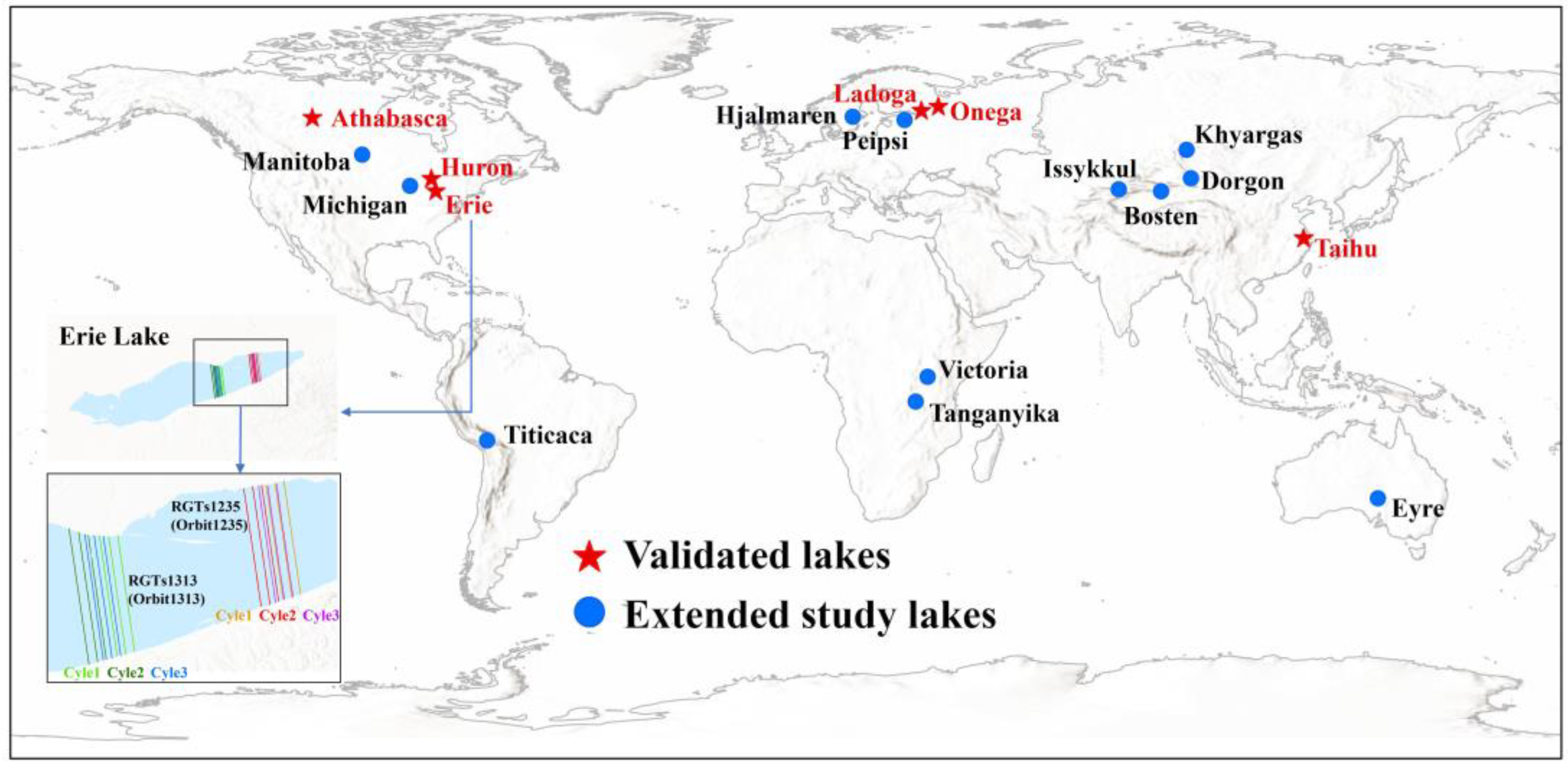
2.1.1. Study Area and Lake Selection

The first group study cases include six validated lakes that have in-situ measurements of water level. The selection criteria for validated lakes include different numbers of ICESat-2 orbital observations, sizes, and locations. These lakes are mostly located in North America and Europe, due to the easier access to gauging stations. Taihu Lake in Asia (East China) was selected as a special validation case because of its relatively smaller area and lower number of ICESat-2 orbits. In addition to the validated lakes, another 12 study lakes, distributed across various continents and without in-situ data, are selected for demonstrating the applicability of this synthesis method. Figure 1 shows the location of the 18 lakes selected for this work, with an example of lake level measured by two-orbit measurements of ICESat-2.

2.1.2. ICESat-2 Altimetry Data

ICESat-2 was launched on 15 September 2018, with the primary goal of measuring Earth’s surface height change along the global Reference Ground Track (RGT) [7]. The ICESat-2 mission along 1387 different RGTs (termed orbits hereafter) acquires finer footprints (<17 m diameter) than ICESat and other radar altimeters. Each orbit has a 91-day repeat cycle [29]. In this paper, the fifth version of the ICESat-2 level-3A product of inland surface water height (ATL13_V5), from 1 December 2018 to 30 November 2021, was collected and processed to derive the water level time series for study lakes. The ATL13_V5, derived from the ICESat-2 ATLAS sensor, provides along-track surface height over inland water bodies, including lakes, reservoirs, bays, estuaries, and rivers [29]. For each study lake, we chose the median value of along-track ICESat-2 elevation retrievals as the water level of each piece of observation data for every orbit due to its statistical robustness against outliers.

2.1.3. Auxiliary Data

Daily in-situ water level observations were collected for evaluation of the synthesized results for six validated lakes (Huron Lake, Erie Lake, Athabasca Lake, Ladoga Lake, Onega Lake, and Taihu Lake) in Section 3.1. Huron Lake and Erie Lake have in-situ lake water levels accessed from NOAA Great Lakes Environmental Research Laboratory (https://www.glerl.noaa.gov/data/wlevels/ (accessed on 1 January 2021)). The gauged water level of Athabasca Lake was received from Historical Hydrometric Data by the government of Canada (https://wateroffice.ec.gc.ca/mainmenu/historical_data_index_e.html (accessed on 1 January 2021)). For Ladoga Lake and Onega Lake, the in-situ water levels were obtained from the Information System on Water Resources and Water Management of the Russian River Basins (http://gis.vodinfo.ru/ (accessed on 1 January 2021)). Validation data of Taihu Lake were gathered from the China Lake-Watershed Science Data Center (http://lake.geodata.cn/ (accessed on 1 January 2021)). The HydroLAKES dataset was used to define study lake boundaries [30].

2.2. Methods

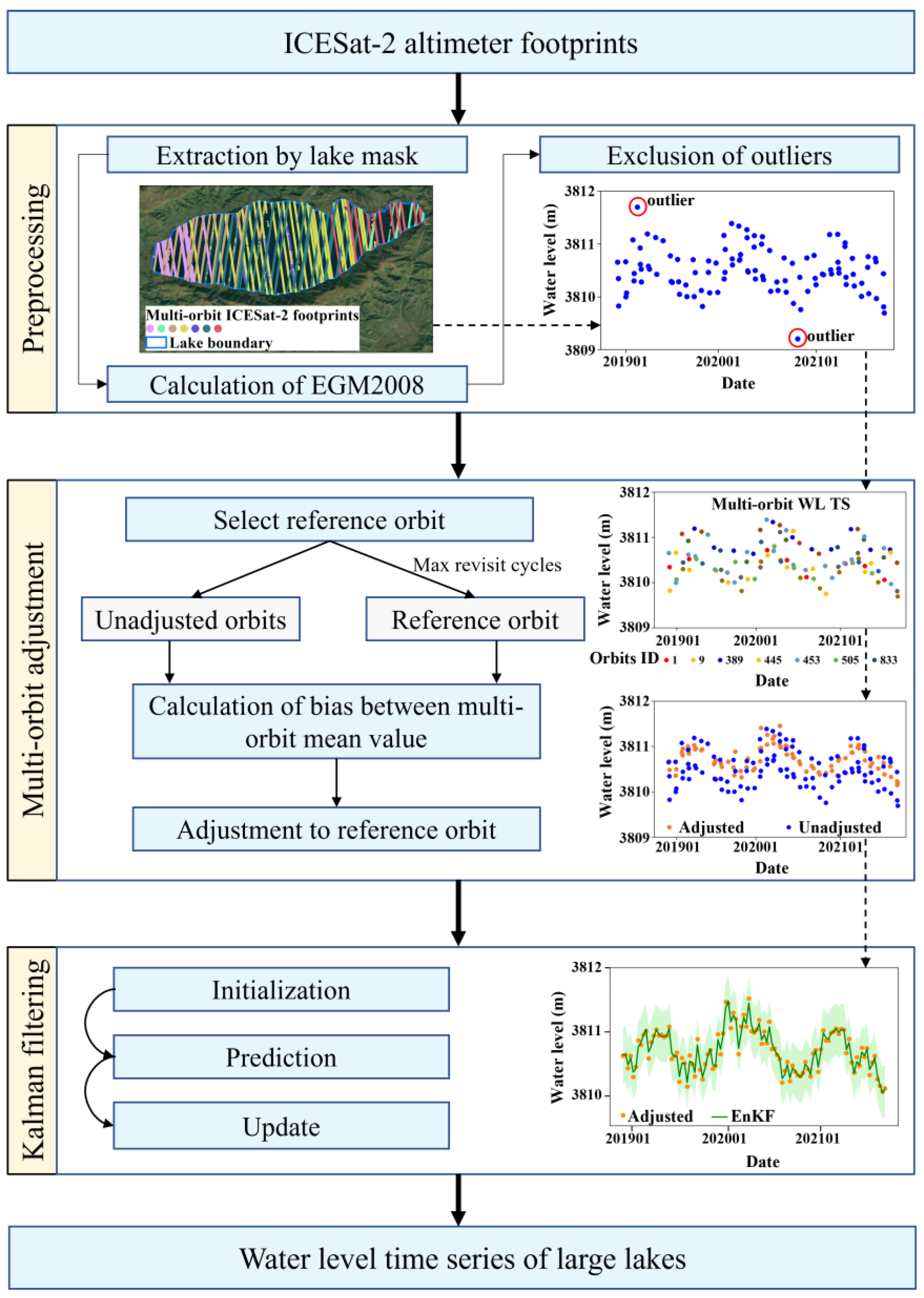
2.2.1. Preprocessing of Lake Level Derived from ICESat-2

In the preprocessing procedure, the water level time series for each study lake was generated based on three steps: altimetry footprint extraction by lake mask, calculation of EGM2008 geoid height, and exclusion of water surface height outliers (Figure 2). Firstly, key variables of each altimetry footprint, including coordinates, date time, orthometric height, geoid value, etc., were derived from the ATL13_V5 altimeter product, and then, the on-lake footprints were extracted by using the HydroLAKES lake boundary as a water mask. Secondly, the EGM2008 geoid value was recalculated by the National Geospatial-Intelligence Agency tool (National Geospatial-Intelligence Agency, Springfield, IL, USA, https://earth-info.nga.mil/ (accessed on 1 January 2020)), aiming to improve the orthometric heights by subtracting geoid heights from ellipsoidal heights [13]. Finally, the method of normalized median absolute deviation [31] was used to remove outliers of on-lake footprint heights for each observation date. Further, the median water level was calculated from the filtered footprint heights of each orbit before the multi-orbit adjustment step.

2.2.2. Densification by Synthesizing Multi-Orbit Data

The multi-orbit adjustment aims to densify the water level time series of lakes by combining multiple orbits (on different observation dates) of ICESat-2 data. First, the reference orbit with maximum repeat cycles was selected as the baseline for adjustment reference. Secondly, the remaining orbits were adjusted (termed as unadjusted orbits) with systematic height biases against the baseline orbit, as shown in Figure 2. Then, adjustment value of lake level biases between unadjusted orbits and the reference orbit was calculated based on the mean of paired height differences between the two orbits for each repeat cycle. Finally, all orbits of the lake level series were adjusted to the reference orbit by reducing their systematic height bias to synthesize the multi-orbit water level time series.

2.2.3. Kalman Filtering Optimization

In this study, the ensemble Kalman filtering (EnKF) is applied to optimize the synthesized water level series after multi-orbit adjustment in the last step (Figure 2). EnKF can be viewed as an optimized version of the Kalman filter (KF) introduced by Evensen [32], which is a Monte Carlo-based implementation of the KF for extremely high-dimensional, possibly nonlinear, and non-Gaussian state estimation problems [33]. In contrast to the standard KF method [34], one of the most notable contributions of EnKF is the optimized probability density function in time that is achieved by advancing each member of the ensemble. The EnKF has been successfully used for geodetic applications and hydrological data assimilation. Further, EnKF has a much lower computation cost, since a rather limited number of model states is usually sufficient for reasonable statistical convergence. As shown in Figure 2, the EnKF approach includes an initialization step, prediction step, and update step. The key steps of the EnKF are introduced in the following Equations (1)–(6) (refer to Houtekamer [35]).
X i ( 0 ) = X b + η ,   for   i = 1 , N
In the initialization step (1), where   X b is the ensemble of size N at the initial time, η is the randomly drawn from a normal distribution with zero mean and covariance of the prior guess.
X i ( t + Δ t ) = F ( X i ( t ) ) + Δ t ζ ,   for   i = 1 , N
In the prediction step (2), X i ( t + Δ t ) is each propagated ensemble member moved forward using a stochastic model. F(X) is the function of the stochastic model. ζ is randomly drawn from a normal distribution with zero mean and covariance of the computer model.
K = P f H ( HP f H T + R ) 1
P f = 1 N 1 ( X i ( τ j ) X ¯ ) ( X i ( τ j ) X ¯ ) T    
X i ( τ j ) = X i ( τ j ) + K ( y ( τ j ) + ϵ H ( X i ( τ j ) ) )  
P a = 1 N 1 ( X i ( τ j ) X a ) ( X i ( τ j ) X a ) T  
The update step includes calculating the Kalman gain matrix (Equations (3) and (4)), updating each ensemble member using the perturbed water levels (Equation (5)), and calculating the analysis error covariance matrix (Equation (6)). P f is the evolved covariance of the prior guess, represented by the spread in the evolved ensemble at time τ j . H is the observation matrix relating the state to the observation. R is the error covariance matrices of the observations. X ¯ is the mean of the ensemble. y(x) is a description of how the input water levels relate to the current state. ϵ is randomly drawn from a normal distribution with zero mean and covariance of the computer model. X a is the mean of updated ensemble at time τ j . All filtering steps are implemented on the computer, and we coded the EnKF method in Python based on the source code (https://github.com/rlabbe/Kalman-and-Bayesian-Filters-in-Python (accessed on 1 January 2022)).

2.2.4. Evaluation Metrics

We employed the correlation coefficient (R), root mean square error (RMSE), mean absolute error (MAE), Nash–Sutcliffe efficiency (NSE), and coefficient of variation (CV) to evaluate the performance of the approach for synthesizing multi-orbit ICESat-2 observations. These metrics directly reflect the deviation and dispersion levels of water level time series derived from the ICESat-2 altimeter and gauge stations. Specifically, the evaluation metrics were calculated separately for each lake by the following equations:
R = i = 1 n ( X i X ¯ ) ( Y i Y ¯ ) i = 1 n ( X i X ¯ ) 2 i = 1 n ( Y i Y ¯ ) 2
R M S E = i = 1 n ( X i Y i ) 2 n 1
M A E = i = 1 n | X i Y i | n
N S E = 1 i = 1 n ( X i Y i ) 2 i = 1 n ( Y i Y ¯ ) 2
C V = n i = 1 ( X i X ¯ ) 2 n 1 x ¯ × 100 %
where X i is the water level derived from ICESat-2 for the time i and X ¯ is the mean water level for the study period; Y i is the measured water level from gauge stations for the time i, and Y ¯ is the mean water level for the study period; n represents the number of observations by ICESat-2.

3. Results and Discussion

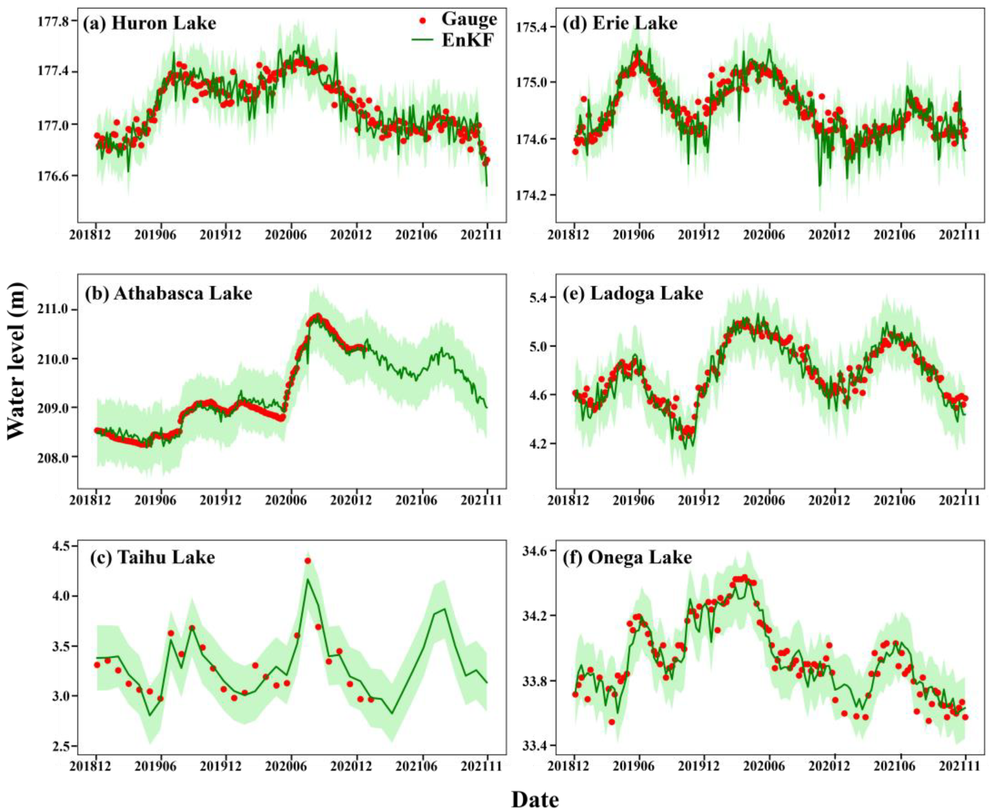
3.1. Validation of Lake Water Level Time Series

The densified and optimized water level time series after orbit adjustment and optimization (termed as EnKF results hereafter) for the six validated lakes are compared against available daily in-situ data (Figure 3). The assessments of EnKF results are detailed in Table 1, showing R of 0.875–0.990, RMSE of 0.078–0.340 m, MAE of 0.064–0.314 m, NSE of −0.143–0.979, and CV of 0.117–10.480. Overall, Figure 3 shows that the processed water levels of the six lakes all have consistent characteristics of annual and inter-annual variations with the in-situ data. The correlation coefficients between the EnKF results and in-situ measurements are all higher than 0.850. In addition, the RMSE and MAE for each lake is less than 12 cm, except for Taihu Lake. It could partially be because the observation time of satellite altimetry and gauged measurement are not completely consistent during the limited validated pairs.
Comparing the evaluation metrics before and after data processing in Table 1 shows that our method can effectively reduce the dispersion degree of the unadjusted water level time series. Take the Ladoga Lake as an example, the improvements in metrics are shown with R being increased from 0.881 to 0.959, NSE being increased from 0.556 to 0.886, RMSE being reduced from 0.155 m to 0.078 m, MAE being reduced from 0.117 m to 0.064 m, and CV being reduced from 6.219 to 5.505. Although the RMSE and MAE of EnKF results for Taihu Lake are larger than those of other validated lakes, our approach similarly optimizes its water level time series from the perspective of evaluation metrics (e.g., the MAE decreased by 2.1 cm). In general, the proposed approach can effectively adjust the water level time series for large lakes measured by multi-orbit ICESat-2 observations.

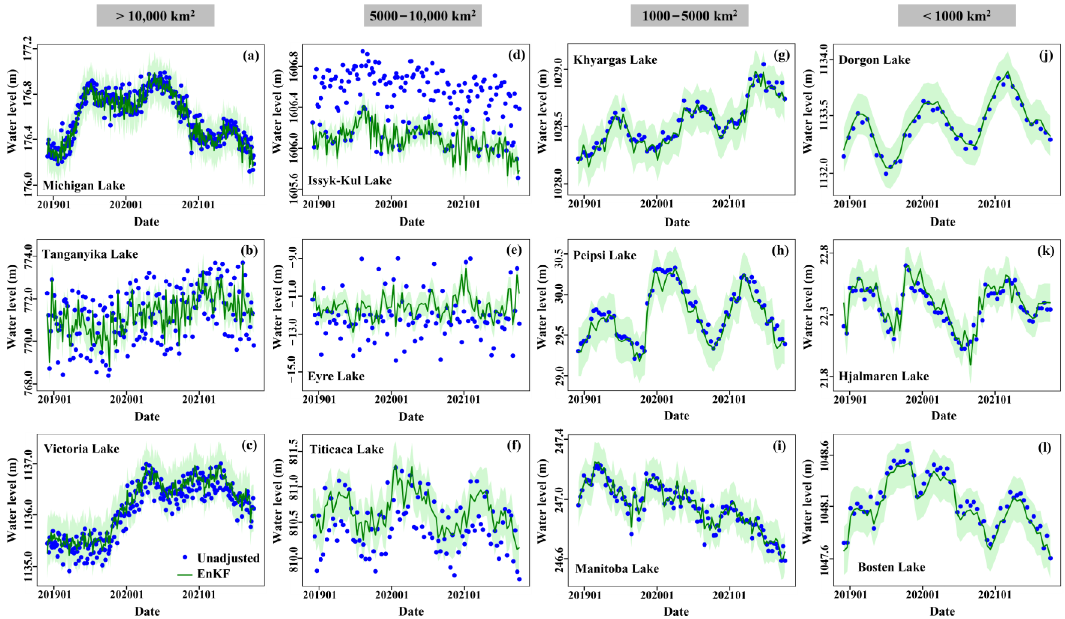
3.2. Lake Level Time Series Synthesized by Multi-Orbit ICESat-2 Footprints

To investigate the feasibility of the approach applied to other lakes, another 12 lakes without gauge stations are selected to derive the densified and optimized results of the water level time series. The 12 lakes with different sizes and geographic locations are employed as extended samples of the approach and divided into four groups according to their sizes, as shown in Figure 4. Overall, similar to the 6 validated lakes, the multi-orbit adjustment, EnKF filtering can result in a more concentrated and reasonable water level series for the 12 lakes. However, there are significant differences in the performances of data densification and optimization among different lake size groups. Lake level time series in the groups of >10,000 km2 and 5000–10,000 km2, by synthesizing multi-orbit ICESat-2 footprints, are denser and more self-organized than the lakes under 5000 km2. For lakes less than 1000 km2, the densification and optimization do not obviously take effect in general.
Meanwhile, the differences in the optimization results of the water level time series for these lakes are shown in Figure 4 and Table 2. Interestingly, the lakes above 5000 km2 in the North American plains (including the Michigan Lake and validated Huron Lake, Erie Lake, and Athabasca Lake) have fewer improvements in data optimization than the lakes in the African Rift Valley, the high mountain regions of Asia and South America (alpine lakes), and the basin region of Oceania. One possible reason could be that these lakes in high-altitudes or basins have larger geoid height differences between orbits than the lakes in plains due to topographic factors. From this perspective, our approach would be more suitable for large lakes with complex topographic features. Further, the more orbits of lakes are covered by ICESat-2, the denser the water level time series that can be derived (Table 2). Therefore, the improvement effect of data densification and optimization in our approach could be stronger for the lakes which have obvious water level differences derived from multi-orbit ICESat-2 observations and with areas over 5000 km2.

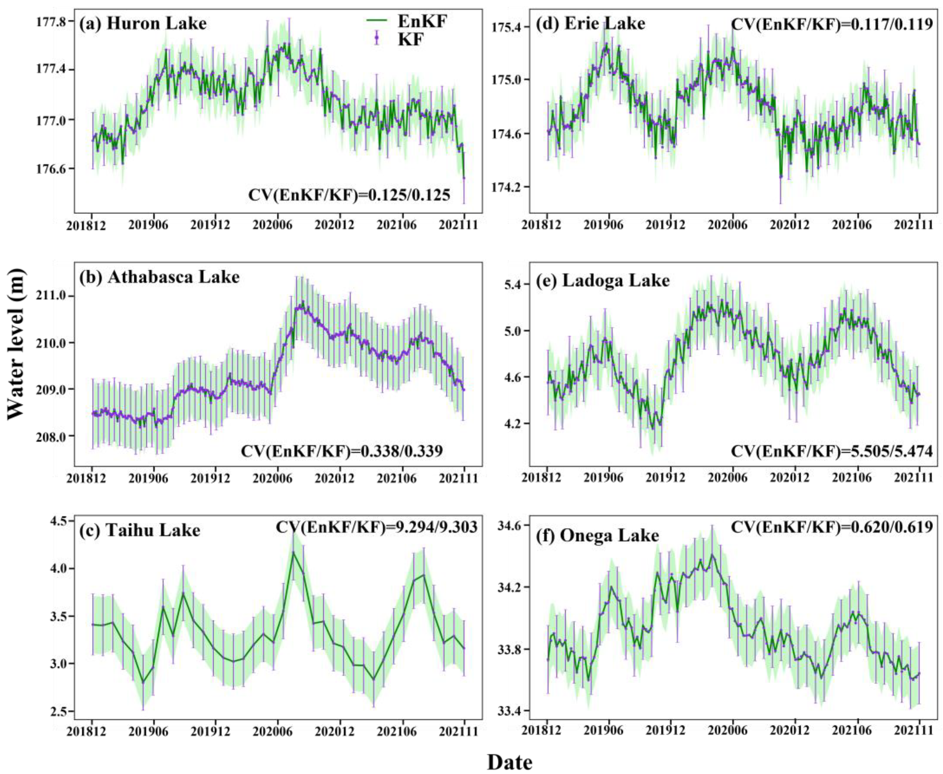
3.3. Comparison of Different Filter Methods

To reveal the influence of the filter step on the synthesized data accuracy in our approach, we compared the performance of the KF and EnKF in densifying and optimizing water level series from the multi-orbit ICESat-2 data. Figure 5 illustrates optimized water level series performances by KF and EnKF for the six validated lakes. Both filter methods perform well in generating smooth and robust trajectories of water level estimates (Figure 5). As an indicator to measure the dispersion degree of water level time series, the CV of the two filter methods is generally consistent (bias range from 0.001% to 0.021%), though EnKF has a slightly better result for most lakes. Further, the CV of six validated lakes is all under 10% (0.125–9.303%). Hence, the step in our approach that has the greatest impact on the densification and optimization of the water level time series could be the multi-orbit adjustment. Generally, the step of the ensemble Kalman filter in our approach only smoothed the water level time series after multi-orbit adjustment but did not densify the final time series.

4. Conclusions

This study proposes an approach of synthesizing multi-orbit ICESat-2 altimetry measurements to densify and optimize the water level time series for large lakes. The approach of synthesizing water level time series has been validated through experiments applied to 6 large lakes with daily in-situ water levels and extended to another 12 ungauged lakes worldwide. The evaluation results demonstrate that our approach can provide an effective solution for densifying the water level series of large lakes covered by multi-orbit ICESat-2 observations. Densified ratio increases as the number of orbits increases, which also indicates that our approach is more suitable for the lakes with more orbital ICESat-2 observations, especially those with an area over 5000 km2.
Our approach has the great potential to obtain accurate estimates of high-frequency water levels based on satellite altimetry. The densified water level series could not only help to indicate the characteristics of the seasonal dynamics of lake water bodies but also be used to investigate the abrupt water level changes due to hydrological extreme events (e.g., floods, droughts, etc.). In the future, quantitative evaluation of water budgets for lakes will be beneficial from densifying the time-series observations by combining multi-mission satellite altimetry (e.g., SARAL/AltiKa, Jason-3, CryoSat-2, Sentinel-3/6). Overall, the optimization processing of more abundant altimeter records will have the potential to improve our understanding of the global water cycle.

Author Contributions

Conceptualization, C.S.; methodology, C.S. and T.C.; software, T.C.; validation, T.C. and P.Z.; formal analysis, T.C., P.Z., C.F. and C.S.; writing, T.C., C.F. and C.S.; visualization, T.C. and C.S.; project administration, C.S.; funding acquisition, C.S. All authors have read and agreed to the published version of the manuscript.

Funding

This work was partly funded by the National Key Research and Development Program of China (Grant No. 2022YFF0711603), the Strategic Priority Research Program of the Chinese Academy of Sciences (Grant No. XDA23100102), National Natural Science Foundation of China (Grant Nos. 42101402, 42277074, 42171421, and 41971403), and Natural Science Foundation of Jiangsu Province (Grant No. BK20210990).

Data Availability Statement

The ICESat-2 altimetry data can be accessed on https://nsidc.org/data/atl13/versions/5 (accessed on 1 January 2019). The lake water mask dataset can be accessed on https://www.hydrosheds.org/products/hydrolakes (accessed on 1 January 2019). The in-situ lake water levels employed in the validation section can be accessed from https://www.glerl.noaa.gov/data/wlevels/ (accessed on 1 January 2021), https://wateroffice.ec.gc.ca/mainmenu/historical_data_index_e.html (accessed on 1 January 2021), http://gis.vodinfo.ru/ (accessed on 1 January 2021), and http://lake.geodata.cn/ (accessed on 1 January 2021).

Acknowledgments

We are grateful to the National Aeronautics and Space Administration for providing ICESat-2 data (https://nsidc.org/data/atl13/versions/5 (accessed on 1 January 2019)), Lehner and Grill for providing the HydroLAKES product (https://www.hydrosheds.org/products/hydrolakes (accessed on 1 January 2019)).

Conflicts of Interest

The authors declare no conflict of interest.

References

  1. Crétaux, J.F.; Arsen, A.; Calmant, S.; Kouraev, A.; Vuglinski, V.; Bergé-Nguyen, M.; Maisongrande, P. SOLS: A lake database to monitor in the Near Real Time water level and storage variations from remote sensing data. Adv. Space Res. 2011, 47, 1497–1507. [Google Scholar] [CrossRef]
  2. Song, C.; Huang, B.; Richards, K.; Ke, L.; Hien Phan, V. Accelerated lake expansion on the Tibetan Plateau in the 2000s: Induced by glacial melting or other processes? Water Resour. Res. 2014, 50, 3170–3186. [Google Scholar] [CrossRef] [Green Version]
  3. Schwatke, C.; Dettmering, D.; Bosch, W.; Seitz, F. DAHITI–an innovative approach for estimating water level time series over inland waters using multi-mission satellite altimetry. Hydrol. Earth Syst. Sci. 2015, 19, 4345–4364. [Google Scholar] [CrossRef] [Green Version]
  4. Busker, T.; de Roo, A.; Gelati, E.; Schwatke, C.; Adamovic, M.; Bisselink, B.; Cottam, A. A global lake and reservoir volume analysis using a surface water dataset and satellite altimetry. Hydrol. Earth Syst. Sci. 2019, 23, 669–690. [Google Scholar] [CrossRef] [Green Version]
  5. Li, X.; Long, D.; Huang, Q.; Han, P.; Zhao, F.; Wada, Y. High-temporal-resolution water level and storage change data sets for lakes on the Tibetan Plateau during 2000–2017 using multiple altimetric missions and Landsat-derived lake shoreline positions. Earth Syst. Sci. Data 2019, 11, 1603–1627. [Google Scholar] [CrossRef] [Green Version]
  6. Papa, F.; Crétaux, J.F.; Grippa, M.; Robert, E.; Trigg, M.; Tshimanga, R.M.; Calmant, S. Water resources in Africa under global change: Monitoring surface waters from space. Surv. Geophys. 2022, 43, 1–51. [Google Scholar]
  7. Neumann, T.A.; Martino, A.J.; Markus, T.; Bae, S.; Bock, M.R.; Brenner, A.C.; Thomas, T.C. The Ice, Cloud, and Land Elevation Satellite–2 Mission: A global geolocated photon product derived from the advanced topographic laser altimeter system. Remote Sens. Environ. 2019, 233, 111325. [Google Scholar] [CrossRef]
  8. Thomas, T.C.; Luthcke, S.B.; Pennington, T.A.; Nicholas, J.B.; Rowlands, D.D. ICESat-2 Precision Orbit Determination. Earth Space Sci. 2021, 8, e2020EA001496. [Google Scholar] [CrossRef]
  9. Bae, S.; Helgeson, B.; James, M.; Magruder, L.; Sipps, J.; Luthcke, S.; Thomas, T. Performance of ICESat-2 precision pointing determination. Earth Space Sci. 2021, 8, e2020EA001478. [Google Scholar] [CrossRef]
  10. Ryan, J.C.; Smith, L.C.; Cooley, S.W.; Pitcher, L.H.; Pavelsky, T.M. Global characterization of inland water reservoirs using ICESat-2 altimetry and climate reanalysis. Geophys. Res. Lett. 2020, 47, e2020GL088543. [Google Scholar] [CrossRef]
  11. Cooley, S.W.; Ryan, J.C.; Smith, L.C. Human alteration of global surface water storage variability. Nature 2021, 591, 78–81. [Google Scholar] [CrossRef] [PubMed]
  12. Feng, Y.; Zhang, H.; Tao, S.; Ao, Z.; Song, C.; Chave, J.; Fang, J. Decadal Lake Volume Changes (2003–2020) and Driving Forces at a Global Scale. Remote Sens. 2022, 14, 1032. [Google Scholar] [CrossRef]
  13. Luo, S.; Song, C.; Ke, L.; Zhan, P.; Fan, C.; Liu, K.; Zhu, J. Satellite laser altimetry reveals a net water mass gain in global lakes with spatial heterogeneity in the early 21st century. Geophys. Res. Lett. 2022, 49, e2021GL096676. [Google Scholar] [CrossRef]
  14. Xu, N.; Ma, Y.; Wei, Z.; Huang, C.; Li, G.; Zheng, H.; Wang, X.H. Satellite observed recent rising water levels of global lakes and reservoirs. Environ. Res. Lett. 2022, 17, 074013. [Google Scholar] [CrossRef]
  15. Xu, N.; Zheng, H.; Ma, Y.; Yang, J.; Liu, X.; Wang, X. Global estimation and assessment of monthly lake/reservoir water level changes using ICESat-2 ATL13 Products. Remote Sens. 2021, 13, 2744. [Google Scholar] [CrossRef]
  16. Scherer, D.; Schwatke, C.; Dettmering, D.; Seitz, F. ICESat-2 Based River Surface Slope and Its Impact on Water Level Time Series from Satellite Altimetry. Water Resour. Res. 2022, 58, e2022WR032842. [Google Scholar] [CrossRef]
  17. Han, W.; Huang, C.; Gu, J.; Hou, J.; Zhang, Y.; Wang, W. Water Level Change of Qinghai Lake from ICESat and ICESat-2 Laser Altimetry. Remote Sens. 2022, 14, 6212. [Google Scholar] [CrossRef]
  18. Lao, J.; Wang, C.; Nie, S.; Xi, X.; Wang, J. Monitoring and Analysis of Water Level Changes in Mekong River from ICESat-2 Spaceborne Laser Altimetry. Water 2022, 14, 1613. [Google Scholar] [CrossRef]
  19. Liu, C.; Hu, R.; Wang, Y.; Lin, H.; Zeng, H.; Wu, D.; Shao, C. Monitoring water level and volume changes of lakes and reservoirs in the Yellow River Basin using ICESat-2 laser altimetry and Google Earth Engine. J. Hydro-Environ. Res. 2022, 44, 53–64. [Google Scholar] [CrossRef]
  20. Narin, O.G.; Abdikan, S. Multi-temporal analysis of inland water level change using ICESat-2 ATL-13 data in lakes and dams. Environ. Sci. Pollut. Res. 2022, 1–13. [Google Scholar] [CrossRef]
  21. Xie, J.; Li, B.; Jiao, H.; Zhou, Q.; Mei, Y.; Xie, D.; Fu, Y. Water Level Change Monitoring Based on a New Denoising Algorithm Using Data from Landsat and ICESat-2: A Case Study of Miyun Reservoir in Beijing. Remote Sens. 2022, 14, 4344. [Google Scholar] [CrossRef]
  22. Zhang, C.; Lv, A.; Zhu, W.; Yao, G.; Qi, S. Using multisource satellite data to investigate lake area, water level, and water storage changes of terminal lakes in ungauged regions. Remote Sens. 2021, 13, 3221. [Google Scholar] [CrossRef]
  23. Madson, A.; Sheng, Y. Automated Water Level Monitoring at the Continental Scale from ICESat-2 Photons. Remote Sens. 2021, 13, 3631. [Google Scholar] [CrossRef]
  24. Yuan, C.; Gong, P.; Bai, Y. Performance assessment of ICESat-2 laser altimeter data for water-level measurement over lakes and reservoirs in China. Remote Sens. 2020, 12, 770. [Google Scholar] [CrossRef] [Green Version]
  25. Chen, T.; Song, C.; Luo, S.; Ke, L.; Liu, K.; Zhu, J. Monitoring global reservoirs using ICESat-2: Assessment on spatial coverage and application potential. J. Hydrol. 2022, 604, 127257. [Google Scholar] [CrossRef]
  26. Shu, S.; Liu, H.; Beck, R.A.; Frappart, F.; Korhonen, J.; Lan, M.; Xu, M.; Yang, B.; Huang, Y.J.H.; Sciences, E.S. Evaluation of historic and operational satellite radar altimetry missions for constructing consistent long-term lake water level records. Hydrol. Earth Syst. Sci. 2021, 25, 1643–1670. [Google Scholar] [CrossRef]
  27. Thakur, P.K.; Garg, V.; Kalura, P.; Agrawal, B.; Sharma, V.; Mohapatra, M.; Kalia, M.; Aggarwal, S.P.; Calmant, S.; Ghosh, S.J.A.i.S.R. Water level status of Indian reservoirs: A synoptic view from altimeter observations. Adv. Space Res. 2021, 68, 619–640. [Google Scholar] [CrossRef]
  28. Wang, X.; Gong, P.; Zhao, Y.; Xu, Y.; Cheng, X.; Niu, Z.; Luo, Z.; Huang, H.; Sun, F.; Li, X.J.R.S.o.E. Water-level changes in China’s large lakes determined from ICESat/GLAS data. Remote Sens. Environ. 2013, 132, 131–144. [Google Scholar] [CrossRef]
  29. Jasinski, M.; Stoll, J.; Hancock, D.; Robbins, J.; Nattala, J.; Morison, J.; Parrish, C. Algorithm Theoretical Basis Document (ATBD) for along Track Inland Surface Water Data, Release 005. 2021. Available online: https://nsidc.org/sites/default/files/icesat2_atl13_atbd_r005_0.pdf (accessed on 1 January 2022).
  30. Messager, M.L.; Lehner, B.; Grill, G.; Nedeva, I.; Schmitt, O. Estimating the volume and age of water stored in global lakes using a geo-statistical approach. Nat. Commun. 2016, 7, 1–11. [Google Scholar] [CrossRef]
  31. Höhle, J.; Höhle, M. Accuracy assessment of digital elevation models by means of robust statistical methods. ISPRS J. Photogramm. Remote Sens. 2009, 64, 398–406. [Google Scholar] [CrossRef] [Green Version]
  32. Evensen, G. Sequential data assimilation with a nonlinear quasi-geostrophic model using Monte Carlo methods to forecast error statistics. J. Geophys. Res. Ocean. 1994, 99, 10143–10162. [Google Scholar] [CrossRef]
  33. Katzfuss, M.; Stroud, J.R.; Wikle, C.K. Understanding the ensemble Kalman filter. Am. Stat. 2016, 70, 350–357. [Google Scholar] [CrossRef]
  34. Kalman, R.E. A new approach to linear filtering and prediction problems. ASME J. Basic Eng. 1960, 82, 35–45. [Google Scholar] [CrossRef] [Green Version]
  35. Houtekamer, P.L.; Mitchell, H.L. Ensemble kalman filtering. Q. J. R. Meteorol. Soc. A J. Atmos. Sci. Appl. Meteorol. Phys. Oceanogr. 2005, 131, 3269–3289. [Google Scholar] [CrossRef]
Figure 1. Location of the validated lakes (red stars) and extended study lakes (blue bubbles). The insert map of one example lake (Erie Lake) illustrated the measurements of two-orbit ICESat-2 altimetry observations (lines represent the ICESat-2 footprints of two orbits with three revisit cycles).
Remotesensing 15 00780 g001
Figure 2. Flowchart for densifying and optimizing water level time series for large lakes by combining multi-orbit data derived from ICESat-2 altimeter. Solid arrows represent data processing and dashed arrows represent input or output data diagrams.
Remotesensing 15 00780 g002
Figure 3. Comparison of optimized ICESat-2 and gauge-derived water level time series for the six validated lakes including (a) Huron Lake, (b) Athabasca Lake, (c) Taihu Lake, (d) Erie Lake, (e) Ladoga Lake, and (f) Onega Lake. The orthometric ICESat-2 water level time series based on EGM2008 is shifted to the individual reported water level height of the gauge data.
Remotesensing 15 00780 g003
Figure 4. Optimized water level time series of selected lakes derived from multi-orbit ICESat-2 footprints over (a) Michigan Lake, (b) Tanganyika Lake, (c) Victoria Lake, (d) Issyk-Kul Lake, (e) Eyre Lake, (f) Titicaca Lake, (g) Khyargas Lake, (h) Peipsi Lake, (i) Manitoba Lake, (j) Dorgon Lake, (k) Hjalmaren Lake, and (l) Bosten Lake. Blue points represent unadjusted water level time series directly derived from the multi-orbit ICESat-2 observations. The green line represents the time series of lake water levels optimized by multi-orbit adjustment and filtering (EnKF results). The light green range represents the uncertainty of the optimized water level time series.
Remotesensing 15 00780 g004
Figure 5. Comparison of water level series of lakes in different sizes by the two Kalman filter methods (KF and EnKF) over (a) Huron Lake, (b) Athabasca Lake, (c) Taihu Lake, (d) Erie Lake, (e) Ladoga Lake, and (f) Onega Lake.
Remotesensing 15 00780 g005
Table 1. Assessment on the final processed water level results for the validated lakes.
Name Unadjusted/EnKF
Area (km2)R 1RMSE 2MAE 3NSE 4CV 5
Huron59,399.300.846/0.8750.126/0.1080.094/0.0840.639/0.7320.133/0.125
Erie25,767.790.857/0.8810.109/0.0980.079/0.0710.623/0.6940.122/0.117
Athabasca7528.730.986/0.9900.136/0.1160.104/0.0930.971/0.9790.339/0.338
Ladoga17,444.010.881/0.9590.155/0.0780.117/0.0640.556/0.8866.219/5.505
Taihu2329.140.984/0.9120.341/0.3400.335/0.314−0.147/−0.14311.394/10.480
Onega9961.850.906/0.9290.121/0.0870.098/0.0690.738/0.8630.660/0.620
1 Evaluation indicator R represents the correlation coefficient between ICESat-2 extracted water level and measured water level of validated lakes. 2 Evaluation indicator RMSE represents the root mean square error of lake level time series. 3 MAE represents the mean absolute error of lake level time series. 4 NSE represents the Nash–Sutcliffe efficiency between lake level series. 5 Evaluation indicator CV represents the coefficient of variation of lake level time series.
Table 2. Summary of sample lakes and assessment of adjustment results.
NameCountryContinentLongitudeLatitudeArea (km2)Elevation (m)Number of Orbits Densified
Ratio *
DorgonMongoliaAsia93.43147.709370.35112864
HjalmarenSwedenEurope15.77059.239474.3924118
BostenChinaAsia87.04041.969961.84105086
KhyargasMongoliaAsia93.31149.1791383.231029117
PeipsiRussiaEurope27.54558.5473489.0028128
ManitobaCanadaNorth America−98.64550.9044751.052451410
Issyk-KulKyrgyzstanAsia77.26642.4416195.9316011814
TiticacaBoliviaSouth America−69.354−15.8828002.513815139
EyreAustraliaOceania137.305−28.5978026.70−15118
TanganyikaCongoAfrica29.886−6.22432,826.657671814
MichiganAmericaNorth America−86.75744.00757,726.841754229
VictoriaUgandaAfrica32.911−1.09967,166.2211342820
* Densified ratio is the ratio of the total number of EnKF results observations to the number of observations in the reference orbit.
Disclaimer/Publisher’s Note: The statements, opinions and data contained in all publications are solely those of the individual author(s) and contributor(s) and not of MDPI and/or the editor(s). MDPI and/or the editor(s) disclaim responsibility for any injury to people or property resulting from any ideas, methods, instructions or products referred to in the content.

