Article

High Signal-to-Noise Ratio MEMS Noise Listener for Ship Noise Detection

State Key Laboratory of Dynamic Measurement Technology, School of Instrument and Electronics, North University of China, Taiyuan 030051, China
*
Author to whom correspondence should be addressed.
Remote Sens. 2023, 15(3), 777; https://doi.org/10.3390/rs15030777
Submission received: 10 November 2022 / Revised: 10 January 2023 / Accepted: 25 January 2023 / Published: 29 January 2023
(This article belongs to the Special Issue Remote Sensing and Other Geomatics Techniques for Marine Applications)

Abstract

:
Ship noise observation is of great significance to marine environment research and national defense security. Acoustic stealth technology makes a variety of ship noise significantly reduced, which is a new challenge for marine noise monitoring. However, there are few high spatial gain detection methods for low-noise ship monitoring. Therefore, a high Signal-to-Noise Ratio (SNR) MEMS noise listener for ship noise detection is developed in this paper. The listener achieves considerable gain by suppressing isotropic noise in the ocean. The working principle and posterior end signal processing method of the listener are introduced in detail. A gain of 10 dB over the sound pressure detector is obtained by detecting the standard sound source. In addition, the traffic vessel noise monitoring experiment verifies that the listener can detect the ship noise. The results show that the listener has a very broad application prospect in the field of low-noise ship observation.

1. Introduction

Remote monitoring of the radiated noise of various types of aircraft in the ocean is an important measure for maritime surveillance and tactical defense. This long-term ocean monitoring provides a research basis for ocean remote sensing applications, including active sonar and passive sonar [1,2,3]. With the development of acoustic stealth technology, the radiated noise of various ships is significantly reduced, which puts forward new requirements for noise measurement technology. Therefore, it is of great national defense significance to study the measurement method of radiated noise of underwater targets and improve the detection ability of quiet targets. The measurement of ship radiated noise abroad was carried out earlier. In 1969, Wenz et al. analyzed data collected from a Point Sur hydrophone array located approximately 40 km west of Cape Sur, California. This system is now a retired US Navy Sound Surveillance System (SOSUS) receiver [4]. In 1989, D. Ross proposed that, from 1950 to 1975, marine environmental sound levels increased by 15 decibels due to shipping. He further predicted that ship noise levels will only increase by about 5 decibels for the rest of the century [5]. From July 1998 to June 1999, the North Pacific Acoustics Laboratory enhanced the existing ATOC acoustic network by installing a sparse two-dimensional receive array west of Surridge, California. The NPAL array consists of four 20-element vertical arrays with an array aperture of 700 m and a 40-element vertical array with an aperture of 1400 m [6]. In 1999, Curtis et al. collected the time series of the environmental sound spectrum through 13 hydrophones deployed in the North Pacific, focusing on the distribution characteristics of [7]. In 2011, Chapman and Price investigated low-frequency deep ocean environmental noise trends in the Northeast Pacific. They reported trends in low-frequency (10–400 Hz) ambient noise levels and described tests conducted at deep-sea sites in the Northeast Pacific from 1978 to 1986 using multivariate volume arrays [8]. In 2016, Brooker et al. presented ship radiated noise data measured using three hydrophone arrays during a recent sea trial conducted as part of the SONIC project [9].
In order to obtain the necessary array gain, the measurement array of conventional acoustic pressure hydrophones is often a large number of elements when measuring low-noise targets, which results in difficulty in the field deployment and tedious data processing in the later stage. The vector hydrophone can simultaneously measure the sound pressure and vibration velocity of the particle at the same point, thereby effectively suppressing the isotropic noise. At the same time, it has a good low-frequency directivity. Compared with the traditional sound pressure measurement method, the vector hydrophone can obtain a higher far-field measurement Signal-to-Noise Ratio (SNR) under the same test conditions. After the 1970s, vector hydrophones began to be used as receiving transducers for underwater radiation target measurements. In 1983, the Soviet Union developed a vector hydrophone low-noise target detection system, CFAC-496. Then, on this basis, it was improved to the FHA-201 system with better performance. From the late 1980s to the early 1990s, Russia used the TAIIC-8 vector hydrophone sonobuoy noise measurement system to conduct long-term ship radiated noise measurements in the Sea of Japan, Sakhalin Island, and the waters near the Kamchatka Peninsula. The United States also developed the SWALLOW buoy system in the early 1990s and tested it in the waters off California. In 1990, the US Marine Physical Laboratory (MPL) developed two vector hydrophone buoy systems and conducted sea trials in the Atlantic Ocean. In 1995, the vector hydrophone shallow sea target trajectory tracking system SWTR was also developed, and sea trials were carried out. The low-noise measurement system designed with vector hydrophones has become a new development direction of underwater acoustic technology. Some achievements have been made in this field abroad, but most of the research on ship radiated noise measurement in China is still based on single-point acoustic pressure hydrophones or acoustic pressure vertical and horizontal arrays. The research on the application of vector hydrophone technology to ship radiated noise measurement has just started. Harbin Institute of Technology conducted research in this field earlier and carried out research on one-dimensional vector hydrophones during the 8th “Five-Year Plan” period. Five years later, the one-dimensional vector hydrophone was applied to the test of radiated noise measurement for the first time in China. Since 1997, it has carried out research on the three-dimensional vector hydrophone, and has carried out many experiments based on the vector hydrophone noise measurement system.
In 2006, the MEMS vector hydrophone based on the principle of bionics and developed at the North University of China has the advantage of small size and low cost, and has good detection performance for low-frequency signals [10,11]. Later, several others conducted related research to improve the sensitivity of hydrophones [12,13,14,15,16]. Recently, Zhu et al., Shang et al., and Zhang et al. studied the orientation estimation algorithm for MEMS vector hydrophones [17,18,19].
With the emergence of low-noise targets in the ocean, new technologies must be adopted to obtain sufficient spatial gain to detect the noise of ships under low Signal-to-Noise Ratio (SNR) conditions. In order to improve the SNR of measurement, a high SNR MEMS noise listener for ship noise detection is developed for the first time, which is compact, flexible, and has high gain. At the same time, a radiated noise analysis algorithm based on MEMS vector sensor is proposed, which can obtain considerable gain by suppressing isotropic noise.

2. Materials and Methods

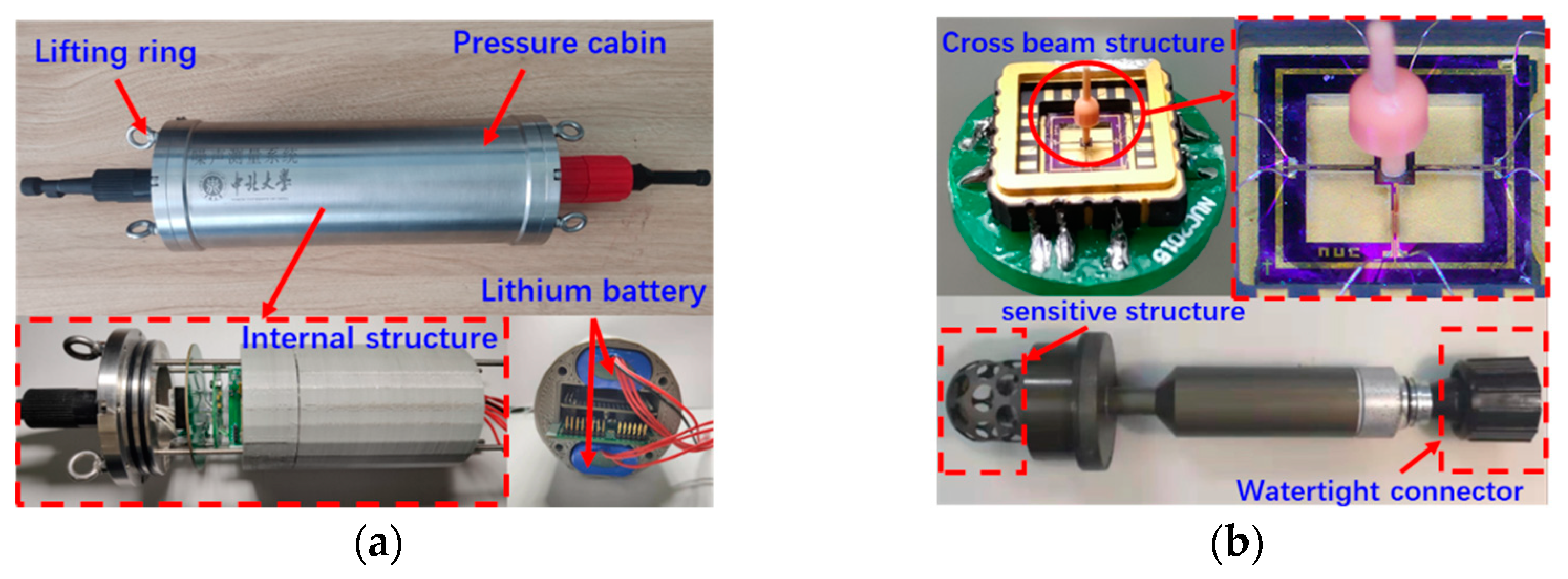
2.1. Composition of MEMS Noise Listener

The MEMS noise listener is mainly composed of a MEMS vector-sensitive probe and an electronic cabin. The overall structure of the listener is shown in Figure 1. The sensitive probe of MEMS vector sensor is connected to the electronic cabin through a watertight connector, and the circuit board and lithium battery are sealed in the electronic cabin. The electronic cabin communicates with the host computer via USB for user control before and after deployment. In order to accurately record oceanic noise, the sampling frequency of the listener is set to 40 k samples/s and the sampling depth is 24 bits. All channels are equipped with high-precision clocks to achieve synchronous sampling. The listener adopts a low-power design, and the equipped lithium battery can ensure that the listener can work continuously for more than 48 h underwater. The working sketch of the MEMS monitor is demonstrated in Figure 2. The listener is placed from the measuring ship to monitor the marine environmental noise. The radiated noise of ships, submarines, and underwater vehicles can be monitored. The monitored data can be transmitted to the aircraft or satellite after being processed on the measurement ship.

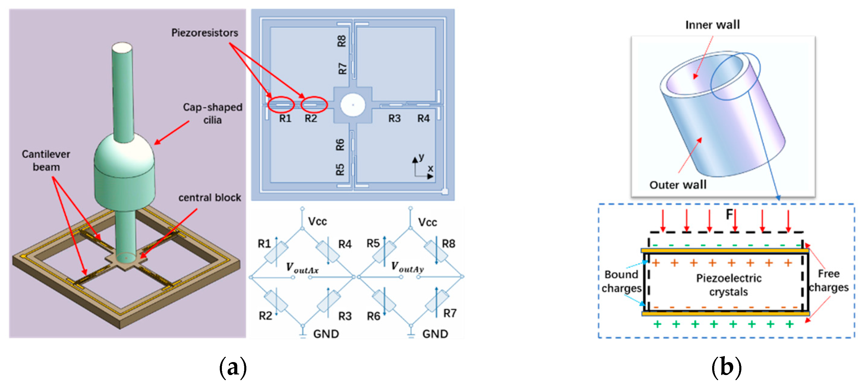
2.2. MEMS Vector-Sensitive Probe Sensing Principle

MEMS vector-sensitive probe contains two vector channels and one acoustic pressure channel. The sensitive structure of the vector channel is shown in Figure 3a. It mainly consists of a cantilever beam with a “cross” structure and a cap-shaped biomimetic cilia [15]. In the figure, the piezoresistive and Wheatstone bridge are enlarged and displayed, and the details are marked with red arrows. The sensitive principle is: when the cilia swing under the action of sound waves, the cantilever beam will deform due to the force. According to the piezoresistive effect, the resistance value of the varistor on the cantilever beam also changes. Finally, the variation of the varistor is converted into a voltage variation output through two Wheatstone bridges [11]. The sensitive structure of the acoustic pressure channel is shown in Figure 3b, which is made of a piezoelectric ceramic tube. The sensitive principle is: when the acoustic pressure acts on the ceramic tube, the inner and outer walls of the ceramic tube will generate charges of opposite polarities, and then output the voltage value through the circuit. After the standing wave tube calibration experiment, the vector channel sensitivity is −182 dB@1 kHz (0 dB~ 1   V / μ Pa ), and the scalar sensitivity is −181 dB (10–1000 Hz). (0 dB~ 1   V / μ Pa ) The sensitivity curve is shown in Figure 4a. The directivity diagram measured at 315 Hz is shown in Figure 4b. The calibration results show that the sensor has good low-frequency performance, the null depth of the “8”-shaped directivity diagram of the two vector channels is more than 30 dB, and the directionality and consistency are good.

3. Measurement Principle of Ship Radiated Noise

3.1. Sound Intensity Estimation Principle

The composite MEMS vector sensor is adopted as a receiving sensor, which can synchronize the acoustic pressure and vibration velocity information at the common measurement receiving points [20]. Through the processing of acoustic pressure and vibration velocity, the active sound intensity can be calculated, and then the isotropic noise can be used to cancel each other to improve the SNR [21,22]. Since the sensor used in this listener is a two-dimensional vector sensor, the following sound field analysis occurs in the case of two-dimensional plane incidence.
The acoustic pressure and vibration velocity signals measured by the composite MEMS vector sensor at the receiving point are Equation (1):
p t = x t v x t = v t c o s θ v y t = v t s i n θ
Among them, θ 0 , 2 π , is the horizontal azimuth angle of the received signal.
Assuming that the sound field satisfies the plane wave Ohm’s law, it can be expressed as Equation (2):
v t = 1 ρ c p t
Substituting Equation (2) into Equation (1) gives
p t = x t v x t = 1 ρ c x t c o s θ v y t = 1 ρ c x t s i n θ
When discussing signal processing problems, the acoustic impedance ρ c in Equation (3) is generally omitted and set to 1 (it cannot be omitted when discussing acoustic problems and physical dimensions are involved). So Equation (3) can be simplified to Equation (4):
p t = x t v x t = x t c o s θ v y t = x t s i n θ
Considering the actual reception situation, the collected signal generally contains a certain amount of noise. Generally, it is approximated as white Gaussian noise, and the actual acquired signal model is
p t = x t + n p t v x t = x t c o s θ + n x t v y t = x t s i n θ + n y t
where n i t i = p , x , y represents noise, which is not related to the signal x t .
Sound intensity is the average sound energy flow per unit area perpendicular to the sound propagation direction, also known as the average sound energy flow density. It can be expressed by the work done by the sound wave per unit time and unit area to the adjacent medium in the propagation direction, shown as Equation (6):
I = 1 T 0 T p t v t d t
For the traditional scalar hydrophone, the vibration velocity v t is calculated by Equation (2), and the noise is also calculated as a part of the signal during the acquisition process. The sound intensity is shown in Equation (7):
I = 1 T 0 T p t 1 ρ c p t d t = 1 T 0 T x t + n p t 2 d t = 1 T 0 T x 2 t + n p 2 t d t
For the vector hydrophone, v t is calculated by the vector sum of v x t and v y t . Assuming that its noise is n v t , uncorrelated with n p t and is uncorrelated with x(t), so it can effectively reduce the interference when calculating the sound intensity, as shown in Equation (8):
I = 1 T 0 T p t v t d t = 1 T 0 T x t + n p t x t + n v t d t = 1 T 0 T x 2 t d t
It can be seen from Equations (7) and (8) that the vector sensor can effectively reduce the interference when calculating the sound intensity. Considering the actual situation, it is less likely to completely eliminate the noise, but using the vector sensor to calculate the sound intensity is obviously effective for reducing isotropic noise.
The complex sound intensity is equivalent to the frequency spectrum of the sound intensity, which often has better applications in engineering. The complex sound intensity can be calculated from the cross-spectrum of sound pressure and vibration velocity. The formulas for calculating the complex sound intensity of the traditional hydrophone and the vector sensor are shown in Equations (9) and (10), respectively.
I p ω = R e 1 ρ c P ω P * ω = X ω 2 + N p ω 2
I v ω = R e P ω V * ω = X ω 2
Like the sound intensity in the time domain, the complex sound intensity calculated by the vector sensor can also effectively improve the SNR. It can be seen from Equations (9) and (10) that the complex sound intensity calculated from the acoustic pressure and vibration velocity output by the vector sensor does not contain noise energy [23]; that is, it has the ability to resist isotropic noise, which is advantageous for signal detection. Through this measurement, isotropic noise is cancelled, which will effectively improve the measurement SNR, so that the original weaker signal can be measured.

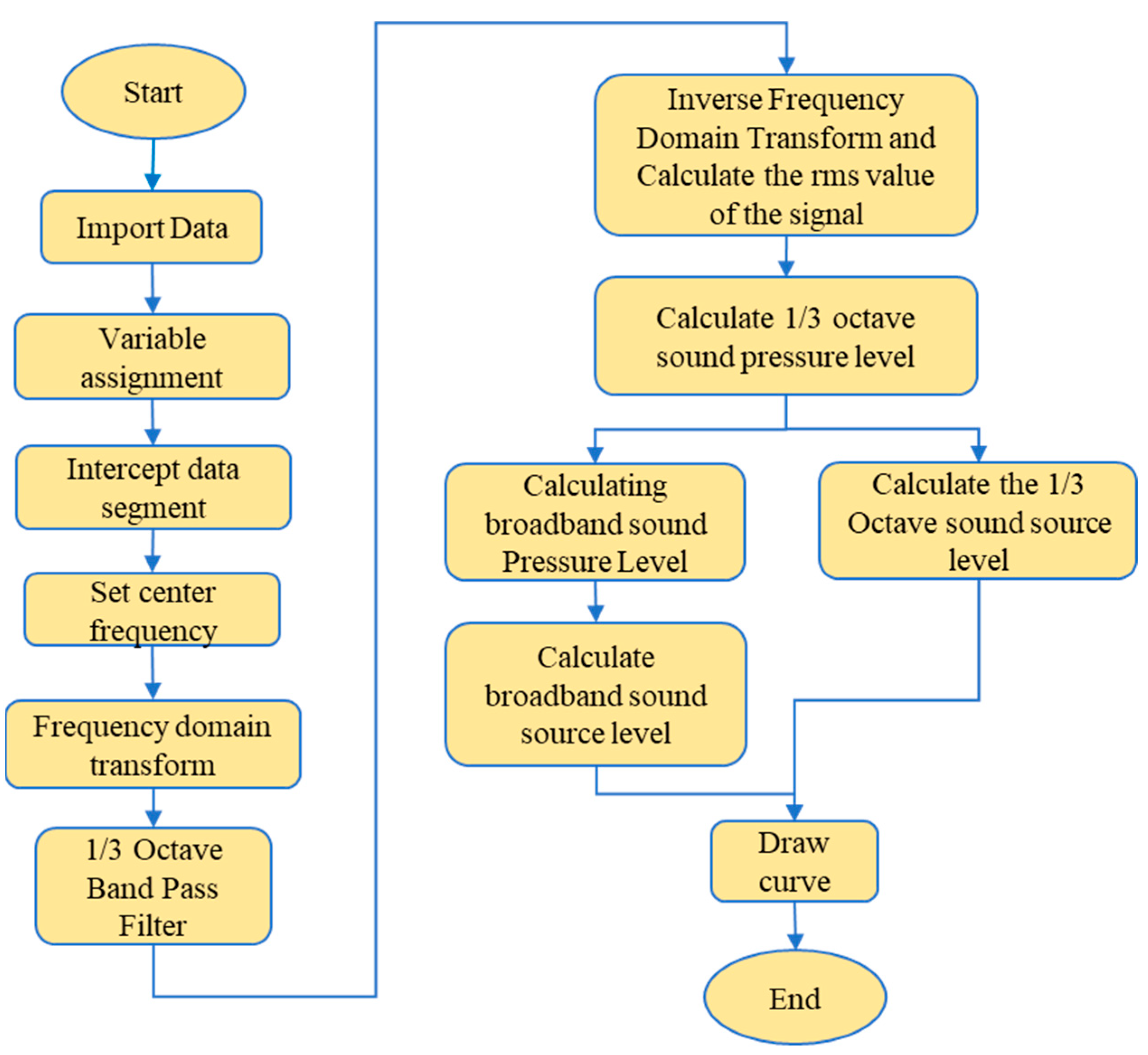
3.2. Radiated Noise Sound Source Level Calculation Method

In the quantitative analysis of target radiation noise, the analysis should focus on parameters such as the line spectrum signal radiated by the target and the acoustic pressure level and sound source level of the broadband signal. The analysis process is shown in Figure 5. First, the power spectrum of the radiated noise signal obtained by the listener at different times is calculated, and the frequency characteristics of the sound source are analyzed. Then, determine the sliding window length and the center frequency of the 1/3 octave bandpass filter. According to the recommendation of the International Organization for Standardization (ISO), select: (1.0, 1.25, 1.6, 2.0, 2.5, 3.15, 4.0, 5.0, 6.3, 8.0) × 10 m Hz , m = 0 , 1 , 2 , [24]. In this paper, according to the working frequency band of the MEMS vector sensor, all 1/3 octave points within 10 Hz-1000 Hz are selected for analysis. Next, the noise signal is frequency domain transformed and filtered using a 1/3 octave bandpass filter. Finally, the filter output is inversely transformed in the frequency domain to obtain the effective value of the signal, and the 1/3 octave band sound pressure level L p i of the radiated noise is calculated through sensitivity compensation. The reference standard of sound pressure is 0   dB ~ 1   μ Pa .
The 1/3 octave frequency band sound source level of ship radiated noise is defined as the frequency band sound pressure level at a distance of 1 m from the equivalent sound center in the direction of the ship’s target sound axis within the specified bandwidth, and can be calculated according to Equation (11):
L p 0 i = L p i + 20 l g d d 0
where L p 0 i is the sound source level in the 1/3 octave frequency band, in dB; L p i is the sound i pressure level of the frequency band in the direction of the sound axis of the output of the ith filter, and away from the sound equivalent center d , in dB; d is the distance of the vector sensor from the equivalent sound center, m; d 0 is the reference distance, d 0 = 1   m .
When analyzing the broadband noise signal in the direction of the target sound axis, the broadband sound pressure level from the equivalent sound center d can be obtained by Equation (12):
L p = 10 l g i = 1 n 10 0.1 L p i
where L p is the broadband sound pressure level, in dB, L p i is the 1/3 octave band sound pressure level, in dB, obtained by the 1/3 octave band-pass filter; n is the number of 1/3 octave filter included in the broadband.
Similarly, the broadband sound source level can be obtained by converting the broadband sound pressure level and distance, as shown in Equation (13):
L p 0 = L p + 20 l g d d 0
where L p 0 is the broadband sound source level, in dB, and L p is the broadband sound pressure level, in dB.
When measured with a 1/3 octave filter bank, the acoustic pressure spectrum level at the center frequency of the No. i filter can be calculated according to Equation (14):
L p s i = L p i 10 l g Δ f i Δ f 0
where L p s i is the acoustic pressure spectrum level of radiation noise, in dB; L p i is the acoustic pressure level of the 1/3 octave frequency band, in dB; Δ f i is i the effective bandwidth of the ith filter, Hz; Δ f 0 is the reference bandwidth, Δ f 0 = 1   Hz .
The acoustic pressure spectrum source level of radiated noise is defined as: in the direction of the sound axis, the acoustic pressure spectrum (density) level at a distance of 1 m from the equivalent sound center, the acoustic pressure spectrum source level can be calculated according to Equation (15):
L p s 0 i = L p s i + 20 l g d d 0
where, L p s 0 i is the acoustic pressure spectrum source level, in dB, and L p s i is the acoustic pressure spectrum level, in dB. where the 1/3 octave frequency band sound pressure level should be calculated according to Equation (16) in combination with the sensitivity of the sensor:
L p i = 20 l g V i V 0 M i K i
where i is the serial number of the 1/3 octave filter; V i is i the output voltage of the ith filter, V; V 0 is the reference voltage, V 0 = 1 V ; M i is the sensor sensitivity at the center frequency of the ith filter, dB, the reference is 1   V / μ Pa ; K i is the electronic system gain at the center frequency of ith filter, in dB.
Important parameters such as frequency band acoustic pressure level, frequency band sound source level, broadband sound pressure level, broadband sound source level and sound-pressure spectrum level of radiated noise can be obtained by Equations (11)–(16). Similarly, 1/3 octave spectrum analysis is performed on the background noise, and its acoustic pressure spectrum level is obtained according to Equation (14). According to the requirements of the national military standard GJB273-87 for the measurement of underwater radiated noise of ships, when the SNR is greater than 10 dB, it is considered that the intensity of ship radiated noise is much greater than the background noise, and the contribution of the background noise can be ignored. When the SNR is greater than 6 dB and less than 10 dB, the calculation results should be corrected according to Table 1, specifically by subtracting the corrected value from the calculated sound pressure level and sound source level. When the SNR is less than 6 dB, it means that the ship radiated noise received by the vector sensor is similar to the environmental noise, and the data is considered invalid and should be discarded.

4. Results

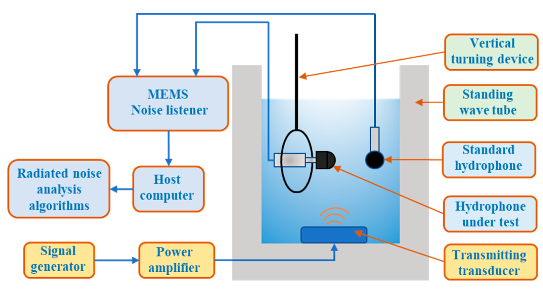
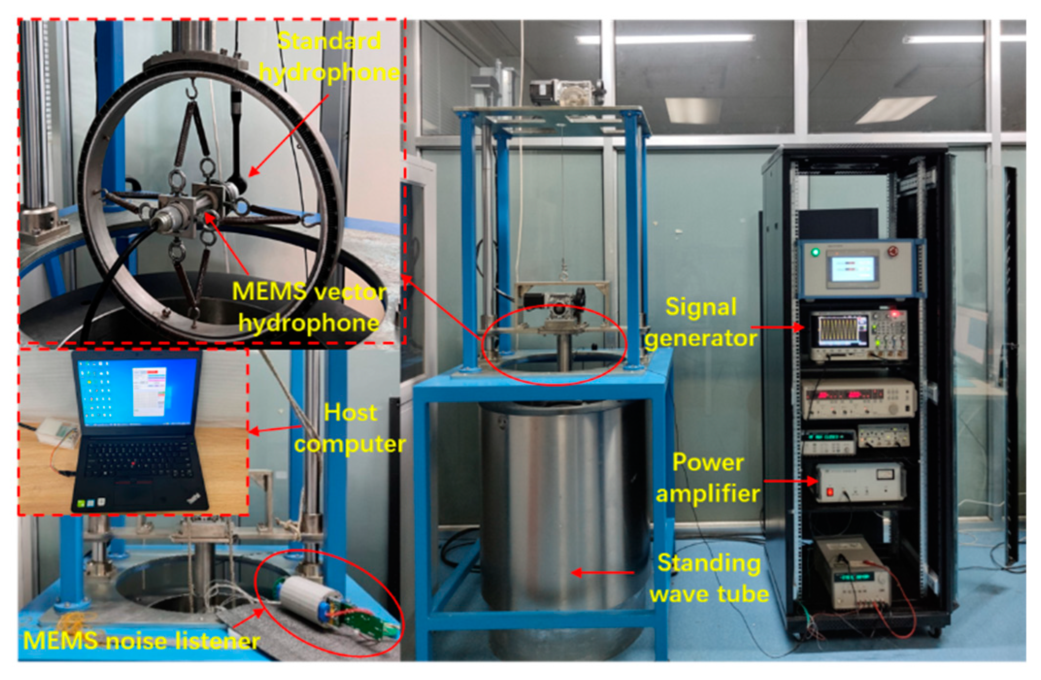
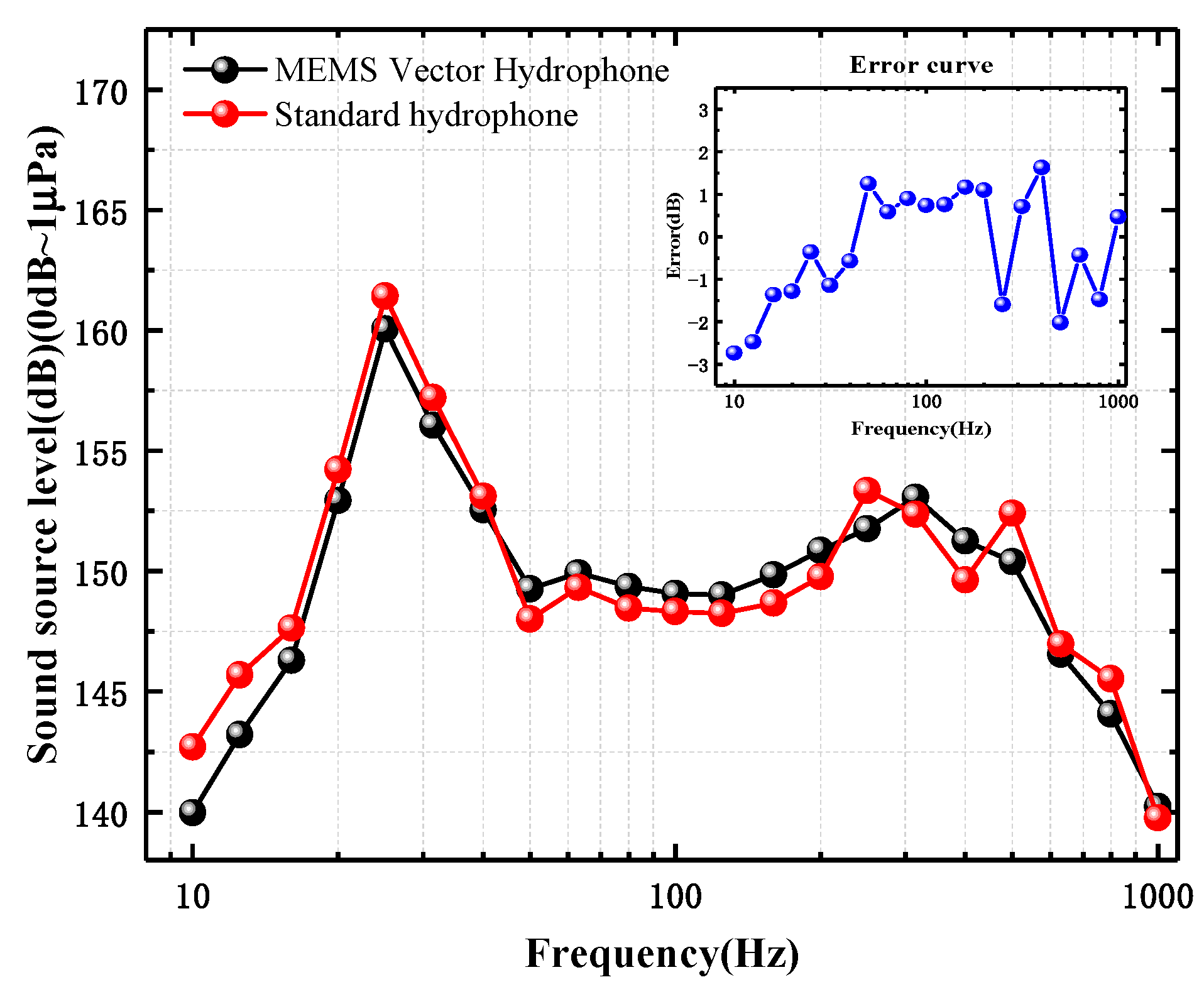
4.1. Error Calibration Experiment

The calibration experiment of the MEMS noise listener was completed in a standing wave tube. The experiment adopted the comparative method to test the error of the listener, using a standard hydrophone as a reference. The experimental equipment is marked with yellow arrows, and the test process is explained with blue arrows in Figure 6. The test process is as follows: First, hang the MEMS vector sensor and the standard hydrophone in the standing wave tube at the same time, and lower the sensors to a position 48 cm away from the sound source through the controller. Then, the 1/3 octave single-frequency signal in the frequency band of 10 Hz-1000 Hz is sequentially transmitted through the sound source at the bottom of the standing wave tube, and the sound signals picked up by the two sensors are collected by the listener at the sampling rate of 40 k samples/s. The test site is shown in Figure 7. The test equipment is marked with red arrows, and the sensor being tested is magnified in the red dotted frame. After the experiment, the radiation noise measurement algorithm is used to analyze and calculate the sound source level of the transmitted signal in turn. The experimental results are shown in Figure 8. The two curves in the figure are the sound source levels measured by the standard hydrophone and the MEMS vector sensor at different frequency points, and the upper right corner is the measurement error. The sound source level measured by the MEMS vector sensor is within 3 dB 0   dB ~ 1   μ Pa of the sound source level measured by the standard hydrophone. The listener is calibrated according to the calibration results in the standing wave tube to reduce the measurement error.

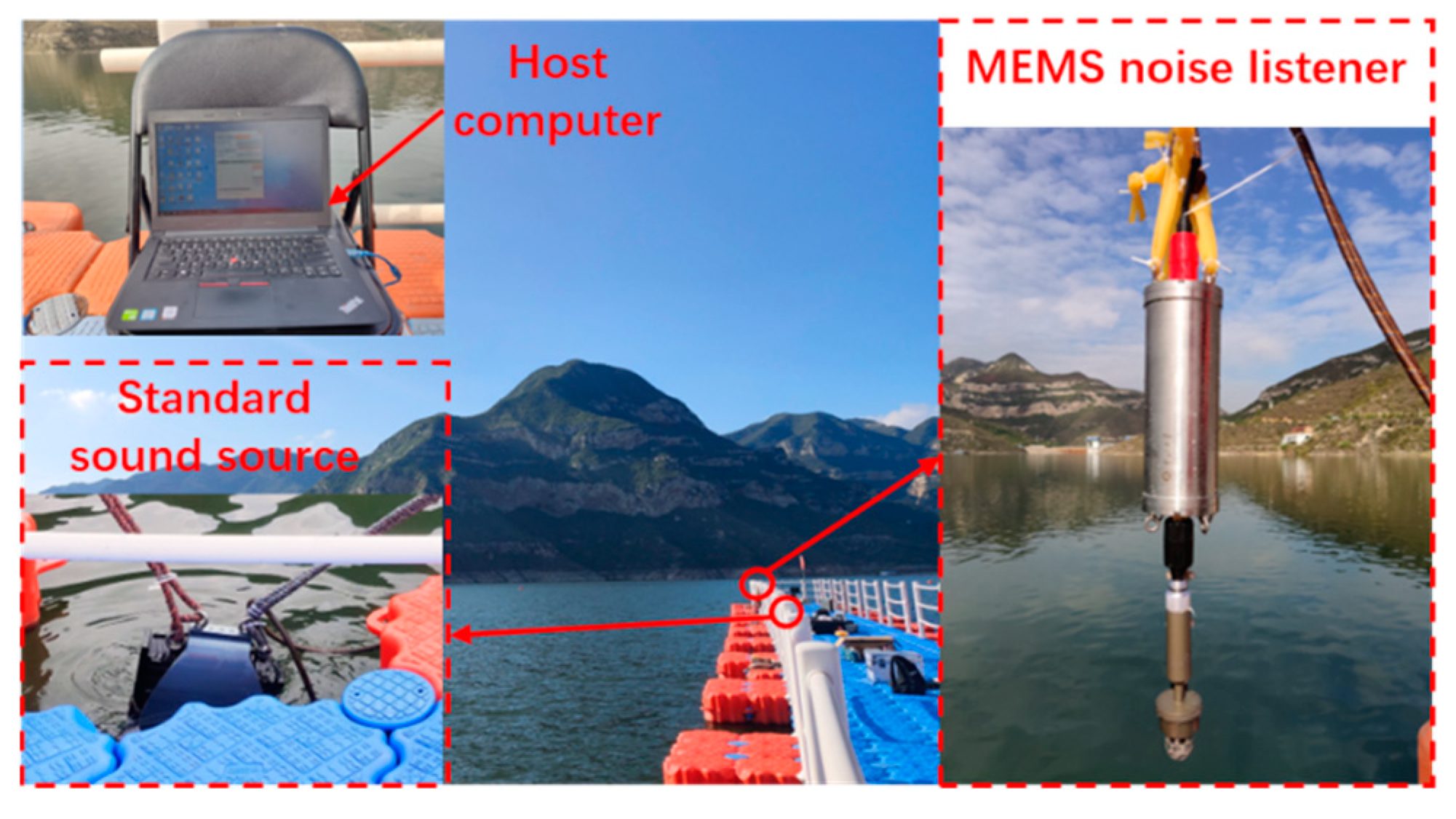
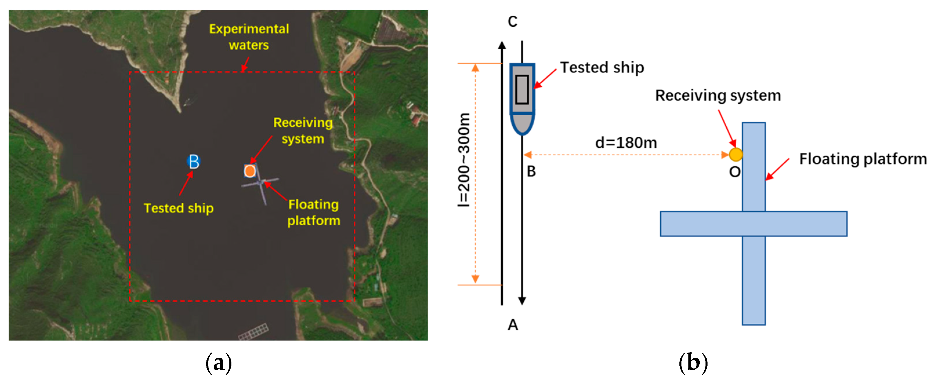
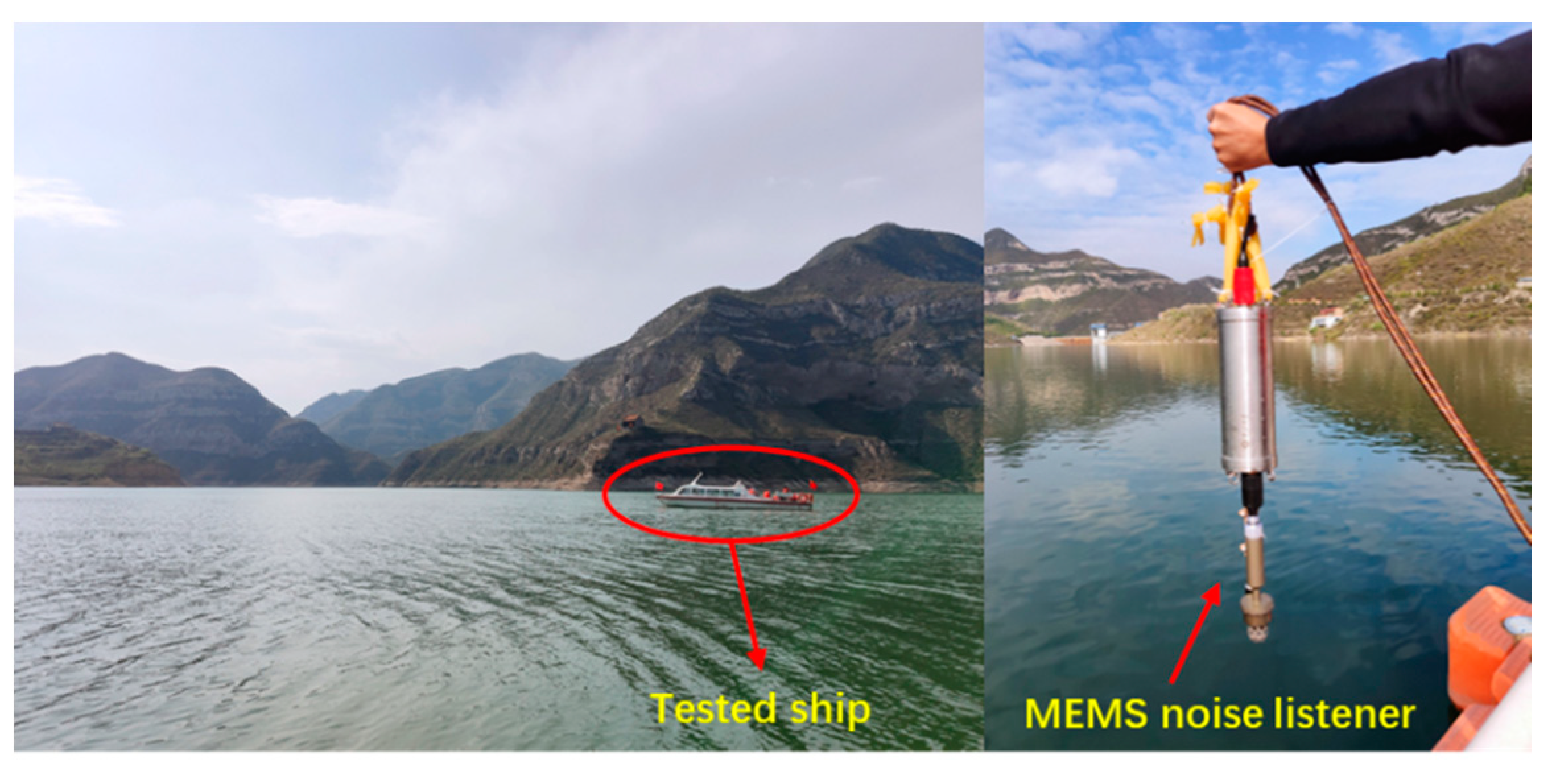
4.2. Outfield Experiment

In order to further verify the monitoring ability of the MEMS noise listener for ship noise, outfield experiments were carried out in the Fenhe No. 2 Reservoir in Taiyuan City. The average depth of the experimental waters is 35 m, and the open area is 1 km2. There is no interference from noise sources such as operating ships in the waters, and the experimental environment is ideal.

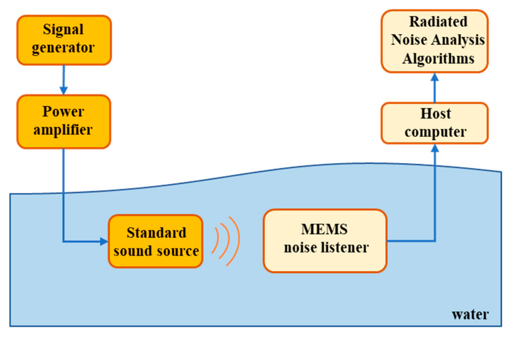
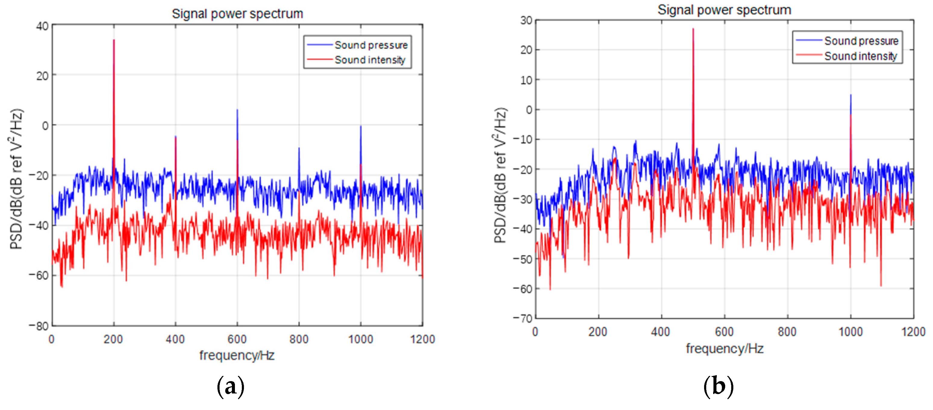
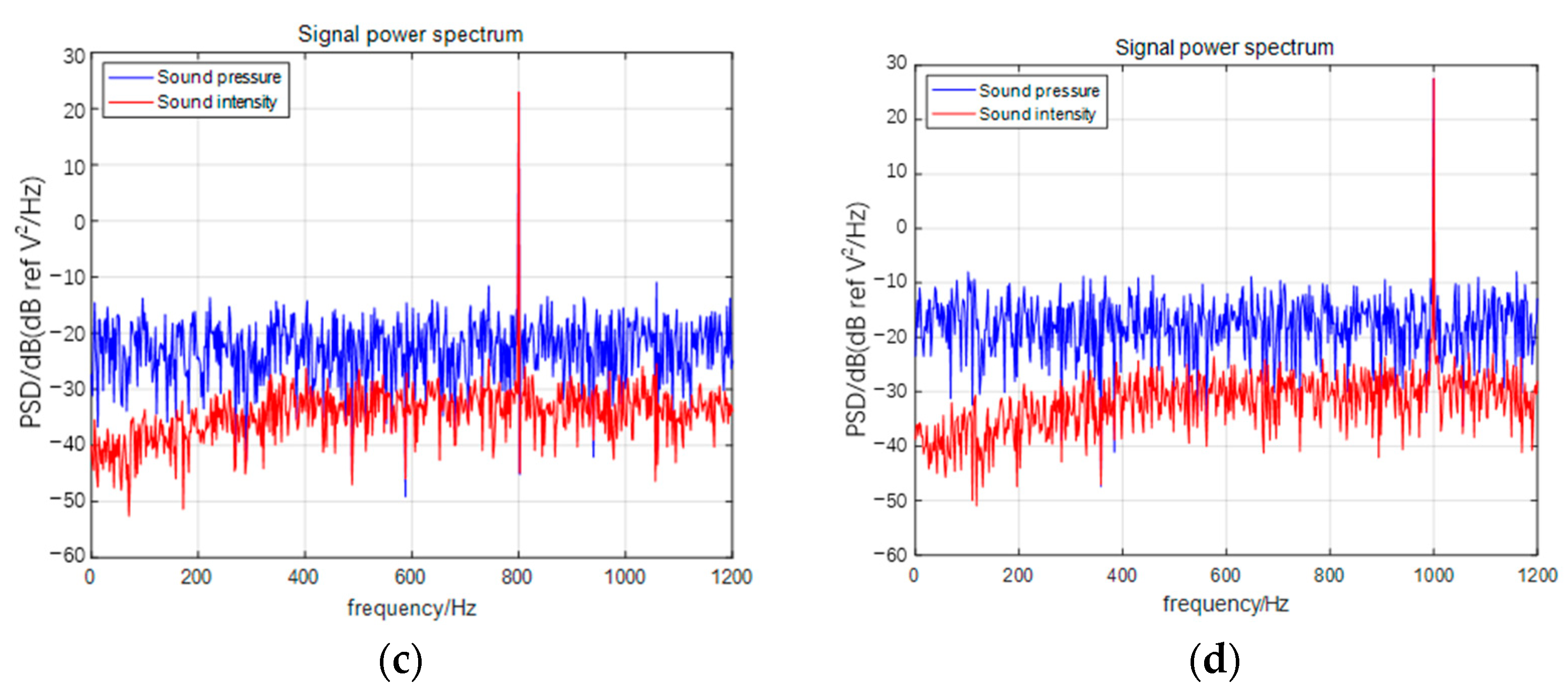
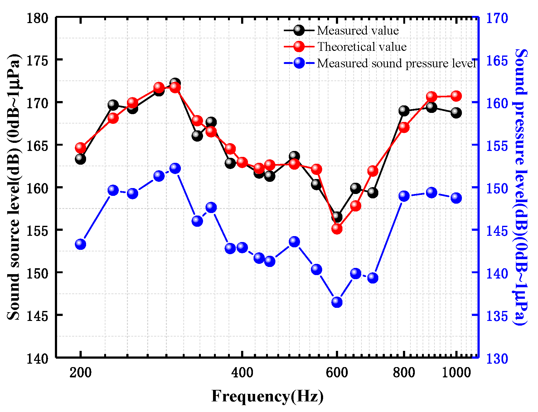
4.2.1. Standard Sound Source Emission Experiment

Standard sound source emission experiments were performed on a cross-shaped floating platform in the center of the reservoir. The transmitter equipment included: mobile power supply, signal generator, power amplifier, and fish-lip transducer. The receiver equipment included: a MEMS noise listener and a computer. Considering that the motion noise will be introduced when the vector sensor moves underwater, a flexible suspension method is used to isolate the motion noise of the system and the motion noise is further eliminated by the baseline drift removal algorithm later [25]. The experimental process is shown in Figure 9. In the picture, the orange box is the transmitting device, and the yellow box is the receiving device. Before the experiment, the listener was controlled by the host computer to start the work with a delay of 15 min, and then the listener was lowered at a depth of 15 m underwater. The transmitting system is built at a distance of 15 m from the receiving end, and the depth of the sound source is consistent with the listener. The experimental site is shown in Figure 10. The red circles in the figure are the location of the transmitting equipment and the receiving equipment respectively, and the details are shown in the red dotted frame. The sound source used in the experiment is an overflow cavity flextensional transducer (model: FM300-19#) driven by rare earth materials. During the experiment, according to the frequency points in the performance parameter table of the fish-lip transducer, the specific frequency points are (200, 230, 250, 280, 300, 330, 350, 380, 400, 430, 450, 500, 550, 600, 650, 700, 800, 900, 1000) Hz. After the experiment, the data were sent back to the computer for analysis and processing through the USB interface. As shown in Figure 11, the sound pressure and sound intensity power spectra of four frequencies of 200 Hz, 500 Hz, 800 Hz, and 1000 Hz are shown, respectively. The blue curves in the figure are acoustic pressure curves, and the red curves are all sound intensity curves. The power spectrum of sound pressure is calculated only by the sound pressure channel, while the sound intensity is calculated by the sound pressure channel and vibration velocity channel of vector sensor. Theoretically, the signal multiplication of multiple channels can suppress uncorrelated noise in each channel to improve the SNR. It can be seen from the figure that under the premise of the same target frequency amplitude, the noise of the sound intensity spectrum is obviously lower than the noise of the sound-pressure power spectrum, and the sound intensity of each frequency point has a gain of at least 10 dB relative to the sound pressure. Figure 12 shows the sound source level test results of the fish-lip transducer. The blue curve in the figure is the sound pressure level at the position of the vector sensor, the black curve is the sound source level restored by the listener according to the test distance, and the red curve is the theoretical sound source level in the fish-lip performance parameter table. The experimental results show that the MEMS noise listener has high SNR gain and can accurately monitor the sound source level of the standard transducer. The maximum measurement error is 2.6 dB.

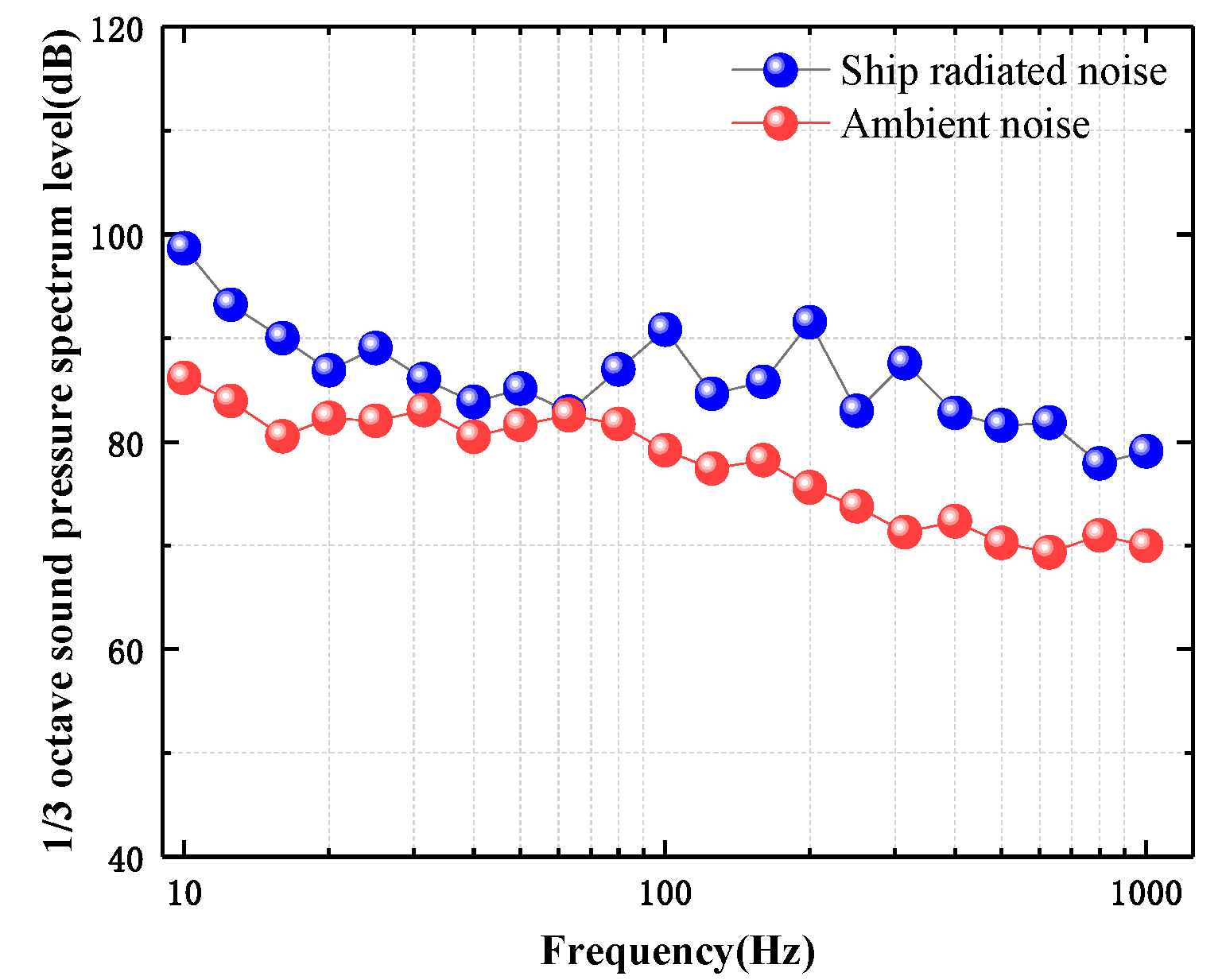
4.2.2. Traffic Ship Radiation Noise Monitoring Experiment

The radiated noise of a small traffic ship in the reservoir is detected by an MEMS noise listener. The red dotted frame in Figure 13a are the experimental waters, and the test site and equipment are marked with red arrows. The monitoring system is again being built on a cross-shaped floating platform. The experimental process is as follows: the listener is started after a delay of 20 min and then lowered at a depth of 5 m underwater. The traffic ship starts to travel back and forth from point A to point C according to the set trajectory in Figure 13b when it reaches a position about 180 m away from the receiving equipment. During the experiment, the precise distance between the transportation ship and the listener was obtained by converting the position information recorded by two GPS locators. The experimental site is shown in Figure 14. The collected radiated noise is analyzed and processed, and a data segment with a length of 20 s near point B, where the target ship is closest to the listener during the voyage, is selected for analysis. Figure 15 shows the acoustic pressure and sound intensity power spectrum of the traffic ship. It can be seen that the sound intensity spectrum obtained by the joint processing of the acoustic pressure and the vibration velocity has a gain of about 4 dB in the low frequency band relative to the sound pressure spectrum. The SNR is about 10.38 dB. Then the background noise before and after the test is analyzed, and the calculated 1/3 octave acoustic pressure spectrum level curves of the background noise and the radiated noise of the traffic ship are shown in Figure 16. According to the correction method in Section 3.2, when the SNR is greater than 10 dB, it is not necessary to correct the sound source level of the target. However, if the sound source level of the monitoring object is too low, or the sound intensity propagated to the location of the listener is too low due to the distance between the monitoring object and the listener, then the ship noise will be submerged in the environmental noise. When the measured SNR is less than 6 dB, the test results are considered invalid. The histogram of the 1/3 octave acoustic pressure level of the traffic ship is shown in Figure 17, and the broadband sound pressure level of the radiated noise of the traffic ship is calculated to be 114.91 dB ( 0   dB ~ 1   μ Pa ). The GPS recording results show that the closest distance between the traffic ship and the listener is 173.6 m, and the restored sound source level is 159.71 dB ( 0   dB ~ 1   μ Pa ). The results show that the MEMS noise listener can monitor underwater targets for a long time, and test results are reliable.

5. Conclusions

This paper presents a high-SNR MEMS noise listener for ship noise detection. A MEMS vector sensor is applied to ocean noise detection for the first time, which makes the listener have the ability to suppress isotropic noise. A higher SNR is obtained by joint processing of sound pressure and vibration velocity. Then, the error caused by the equivalent sound center is effectively reduced by increasing the monitoring distance. The standard sound source experiment obtained a gain of 10 dB higher than the sound-pressure detection method, and the measurement error is within 2.6 dB. The traffic vessel monitoring experiment verifies the ability of the listener to detect ship noise, which is of great significance to ocean noise monitoring. In conclusion, the MEMS ocean noise listener proposed in this paper has the advantages of high SNR, high spatial gain, and small size, which has broad application prospects in the field of low-noise ship monitoring.

Author Contributions

Conceptualization, S.Z.; methodology, D.W.; software, S.Z.; validation, S.Z. and Y.Z.; formal analysis, W.R.; resources, G.Z.; data curation, Y.L.; writing—original draft preparation, S.Z.; writing—review and editing, Y.G. and S.Z.; visualization, L.J.; supervision, W.Z. All authors have read and agreed to the published version of the manuscript.

Funding

This work was supported by National Key Research and Development Project (Grant No. 2019YFC0119800), National Natural Science Foundation of China as National Major Scientific Instruments Development Project (Grant No. 61927807), National Natural Science Foundation of China (Grant No. 52175553), Shanxi Province Basic Research Project (Grant No. 202103021224203), and The Fund for Shanxi ‘1331 Project’ Key Subject Construction and Innovation Special Zone Project.

Data Availability Statement

The data presented in this study are available on request from the corresponding author. The data are not publicly available due to all the research results involved in the data have not yet been published.

Conflicts of Interest

The authors declare no conflict of interest.

References

  1. Fillinger, L.; Sutin, A.; Sedunov, A. Acoustic ship signature measurements by cross-correlation method. J. Acoust. Soc. Am. 2011, 129, 774–778. [Google Scholar] [CrossRef] [PubMed]
  2. Wenz, G.M. Acoustic Ambient Noise in the Ocean: Spectra and Sources. J. Acoust. Soc. Am. 1962, 34, 1936–1956. [Google Scholar] [CrossRef]
  3. Arveson, P.T.; Vendittis, D.J. Radiated noise characteristics of a modern cargo ship. J. Acoust. Soc. Am. 2000, 107, 118–129. [Google Scholar] [CrossRef] [PubMed]
  4. Wenz, G.M. Low-frequency deep-water ambient noise along the Pacific Coast of the United States. US Navy J. Underw. Acoust. 1969, 19, 423–444. [Google Scholar]
  5. Ross, D. Mechanics of underwater noise. J. Acoust. Soc. Am. 1989, 86, 1626. [Google Scholar] [CrossRef]
  6. Colosi, J.A.; Cornuelle, B.D.; Dushaw, B.D.; Dzieciuch, M.A.; Howe, B.M.; Mercer, J.A.; Spindel, R.C.; Worcester, P.F.; NPAL Group. The North Pacific Acoustic Laboratory (NPAL) Experiment. J. Acoust. Soc. Am. 2001, 107, 2384. [Google Scholar] [CrossRef]
  7. Curtis, K.R.; Howe, B.M.; Mercer, J.A. Low-frequency ambient sound in the North Pacific: Long time series observations. J. Acoust. Soc. Am. 1999, 100, 2733. [Google Scholar] [CrossRef]
  8. Chapman, N.R.; Price, A. Low frequency deep ocean ambient noise trend in the Northeast Pacific Ocean. Acoust. Soc. Am. 2011, 129, EL161–EL165. [Google Scholar] [CrossRef]
  9. Brooker, A.; Humphrey, V. Measurement of radiated underwater noise from a small research vessel in shallow water. Ocean. Eng. 2016, 120, 182–189. [Google Scholar] [CrossRef] [Green Version]
  10. Xue, C.; Chen, S.; Zhang, W.; Zhang, B.; Zhang, G.; Qiao, H. Design, fabrication, and preliminary characterization of a novel MEMS bionic vector hydrophone. Microelectron. J. 2007, 38, 1021–1026. [Google Scholar] [CrossRef]
  11. Shang, C.; Xue, C.; Zhang, B.; Xie, B.; Hui, Q. A Novel MEMS Based Piezoresistive Vector Hydrophone for Low Frequency Detection. In Proceedings of the International Conference on Mechatronics & Automation, Harbin, China, 5–9 August 2007. [Google Scholar]
  12. Ji, S.; Zhang, L.; Zhang, W.; Zhang, G.; Wang, R.; Song, J.; Zhang, X.; Lian, Y.; Shang, Z. Design and realization of dumbbell-shaped ciliary MEMS vector hydrophone. Sens. Actuators A Phys. 2020, 311, 112019. [Google Scholar] [CrossRef]
  13. Liu, Y.; Wang, R.; Zhang, G.; Du, J.; Zhao, L.; Xue, C.; Zhang, W.; Liu, J. “Lollipop-shaped” high-sensitivity Microelectromechanical Systems vector hydrophone based on Parylene encapsulation. J. Appl. Phys. 2015, 118, 044501. [Google Scholar] [CrossRef]
  14. Xu, Q.; Zhang, G.; Ding, J.; Wang, R.; Pei, Y.; Ren, Z.; Shang, Z.; Xue, C.; Zhang, W. Design and implementation of two-component cilia cylinder MEMS vector hydrophone. Sens. Actuators A Phys. 2018, 277, 142–149. [Google Scholar] [CrossRef]
  15. Zhu, S.; Zhang, G.J.; Shang, Z.Z.; Yang, X.; Lv, T.; Liang, X.Q.; Zhang, X.Y.; Chen, P.; Zhang, W.D. Design and realization of cap-shaped cilia MEMS vector hydrophone. Measurement 2021, 183, 109818. [Google Scholar] [CrossRef]
  16. Wang, R.; Shen, W.; Zhang, W.; Song, J.; Li, N.; Liu, M.; Zhang, G.; Xue, C.; Zhang, W. Design and implementation of a jellyfish otolith-inspired MEMS vector hydrophone for low-frequency detection. Microsyst. Nanoeng. 2021, 7, 1. [Google Scholar] [CrossRef]
  17. Zhu, S.; Zhang, G.J.; Wu, D.Y.; Liang, X.Q.; Zhang, Y.F.; Lv, T.; Liu, Y.; Chen, P.; Zhang, W.D. Research on Direction of Arrival Estimation Based on Self-Contained MEMS Vector Hydrophone. Micromachines 2022, 13, 236. [Google Scholar] [CrossRef] [PubMed]
  18. Shang, Z.; Zhang, W.; Zhang, G.; Zhang, X.; Ji, S.; Wang, R. Mixed near field and far field sources localization algorithm based on MEMS vector hydrophone array. Measurement 2019, 151, 107109. [Google Scholar] [CrossRef]
  19. Zhang, X.; Zhang, G.; Shang, Z.; Zhu, S.; Zhang, W. Research on DOA Estimation Based on Acoustic Energy Flux Detection Using a Single MEMS Vector Hydrophone. Micromachines 2021, 12, 168. [Google Scholar] [CrossRef]
  20. Zhang, G.; Zhang, L.; Ji, S.; Yang, X.; Wang, R.; Zhang, W.; Yang, S. Design and Implementation of a Composite Hydrophone of Sound Pressure and Sound Pressure Gradient. Micromachines 2021, 12, 939. [Google Scholar] [CrossRef]
  21. Hutt, D.; Hines, P.C.; Rosenfeld, A. Measurement of underwater sound intensity vector. Can. Acoust. 1999, 23, 16–17. [Google Scholar]
  22. Jinglin, D.U.; Zhongcheng, M.A.; Ran, L.I.; Chen, J. Measurement of Background Noise of the South China Sea Based on Vector Hydrophone. J. Test Meas. Technol. 2014, 126, 299–304. [Google Scholar]
  23. Xiao, Y.; Han, Y.; Liu, X. Measurement Technique of Noise Acoustic Intensity Based on Vector Hydrophone. Sci. Technol. Inf. 2009, 3, 45–46. [Google Scholar]
  24. Feng, C.; Zhou, B.K.; Cheng, L.Q.; Huang, J.D.; Weng, H.L. Design of third-octave band FIR digital filters based on MATLAB. J. Fuzhou Univ. 2003, 10, 101–104. [Google Scholar]
  25. Wu, D.Y.; Zhang, G.J.; Zhu, S. A baseline drift removal algorithm based on cumulative sum and downsampling for hydroacoustic signal. Measurement 2023, 207, 112344. [Google Scholar] [CrossRef]
Figure 1. Overall structure diagram of the listener. (a) Electronic cabin structure; (b) MEMS vector sensor package structure.
Remotesensing 15 00777 g001
Figure 2. Working sketch of noise listener.
Remotesensing 15 00777 g002
Figure 3. Sensor sensitivity schematic diagram. (a) Vector channel sensitive structure; (b) Scalar channel sensitive structure.
Remotesensing 15 00777 g003
Figure 4. Calibration result of sensor. (a) Sensitivity curve of sensor; (b) Directivity diagrams of sensor.
Remotesensing 15 00777 g004
Figure 5. Radiated noise analysis process.
Remotesensing 15 00777 g005
Figure 6. Test process diagram of error calibration experiment.
Remotesensing 15 00777 g006
Figure 7. MEMS noise listener calibration site.
Remotesensing 15 00777 g007
Figure 8. Error calibration result diagram.
Remotesensing 15 00777 g008
Figure 9. Schematic diagram of the experimental process.
Remotesensing 15 00777 g009
Figure 10. Experimental site diagram.
Remotesensing 15 00777 g010
Figure 11. Single frequency signal power spectrum. (a) 200 Hz; (b) 500 Hz; (c) 800 Hz; (d) 1000 Hz.
Remotesensing 15 00777 g011aRemotesensing 15 00777 g011b
Figure 12. Standard sound transducer output sound source level.
Remotesensing 15 00777 g012
Figure 13. (a) Experimental water area map; (b) Schematic diagram of the experimental process.
Remotesensing 15 00777 g013
Figure 14. Monitoring site of radiated noise from traffic ship.
Remotesensing 15 00777 g014
Figure 15. Power spectrum of radiated noise from traffic ship.
Remotesensing 15 00777 g015
Figure 16. 1/3 Octave sound pressure spectrum level curve.
Remotesensing 15 00777 g016
Figure 17. 1/3 Octave sound pressure level histogram of traffic ship.
Remotesensing 15 00777 g017
Table 1. Noise level correction table.
SNR (dB)Radiation Noise Level Correction (dB)
100.5
90.5
81.0
71.0
61.0
<6Invalid
Disclaimer/Publisher’s Note: The statements, opinions and data contained in all publications are solely those of the individual author(s) and contributor(s) and not of MDPI and/or the editor(s). MDPI and/or the editor(s) disclaim responsibility for any injury to people or property resulting from any ideas, methods, instructions or products referred to in the content.

