

Global Leaf Chlorophyll Content Dataset (GLCC) from 2003–2012 to 2018–2020 Derived from MERIS and OLCI Satellite Data: Algorithm and Validation


Abstract
:1. Introduction
2. Data and Methods
2.1. Satellite Data
2.1.1. MERIS and OLCI Surface Reflectance Data
2.1.2. MODIS Land Cover Map
2.1.3. The Croft MERIS LCC Dataset
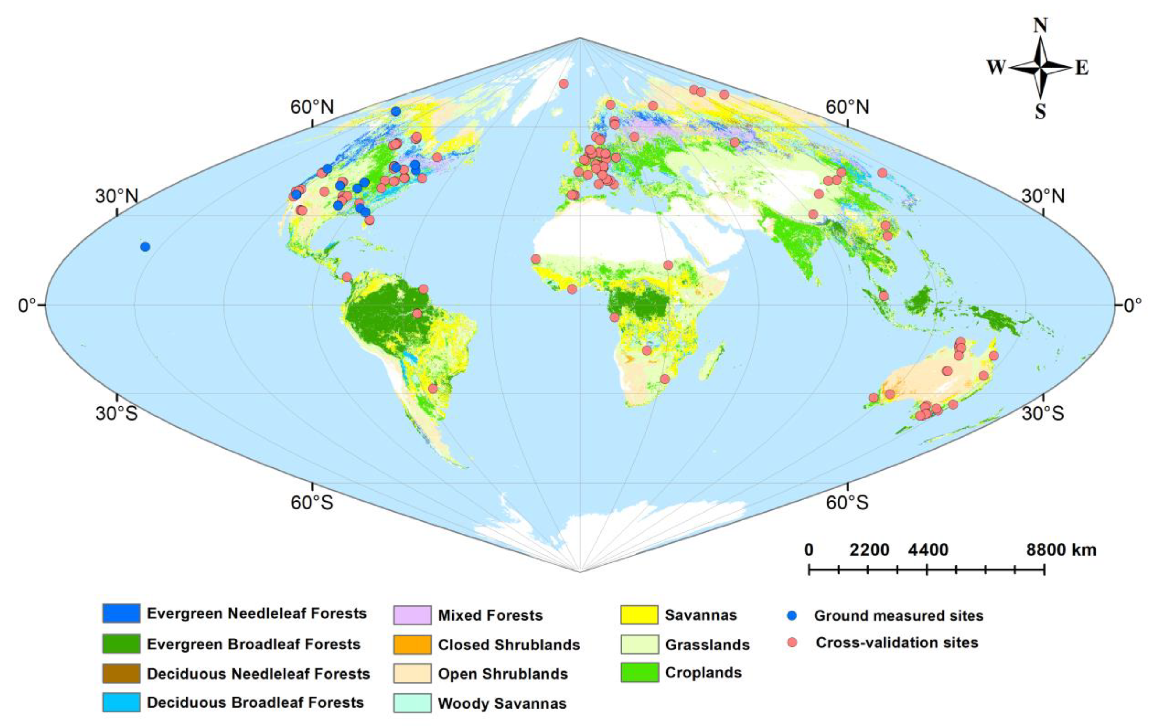
2.2. LCC Field Measurements
2.3. The Cross-Validation Sites
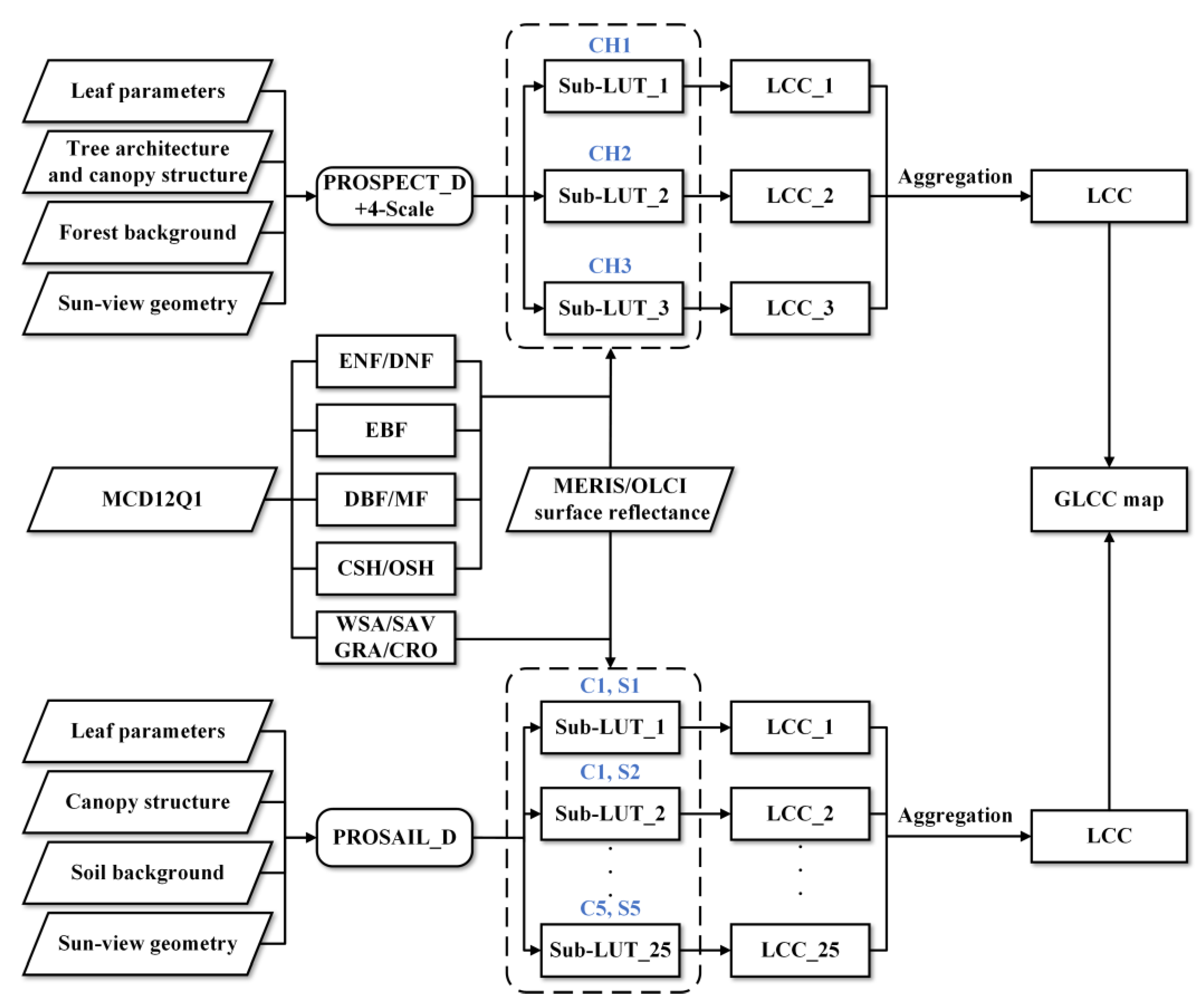
2.4. Algorithm Development
2.4.1. Canopy Reflectance Modeling—PROSAIL_D Model
2.4.2. Canopy Reflectance Modeling—PROSPECT-D and 4-Scale Models
2.4.3. Deriving Leaf Chlorophyll Content
2.5. Validation and Evaluation of the GLCC Dataset
3. Results
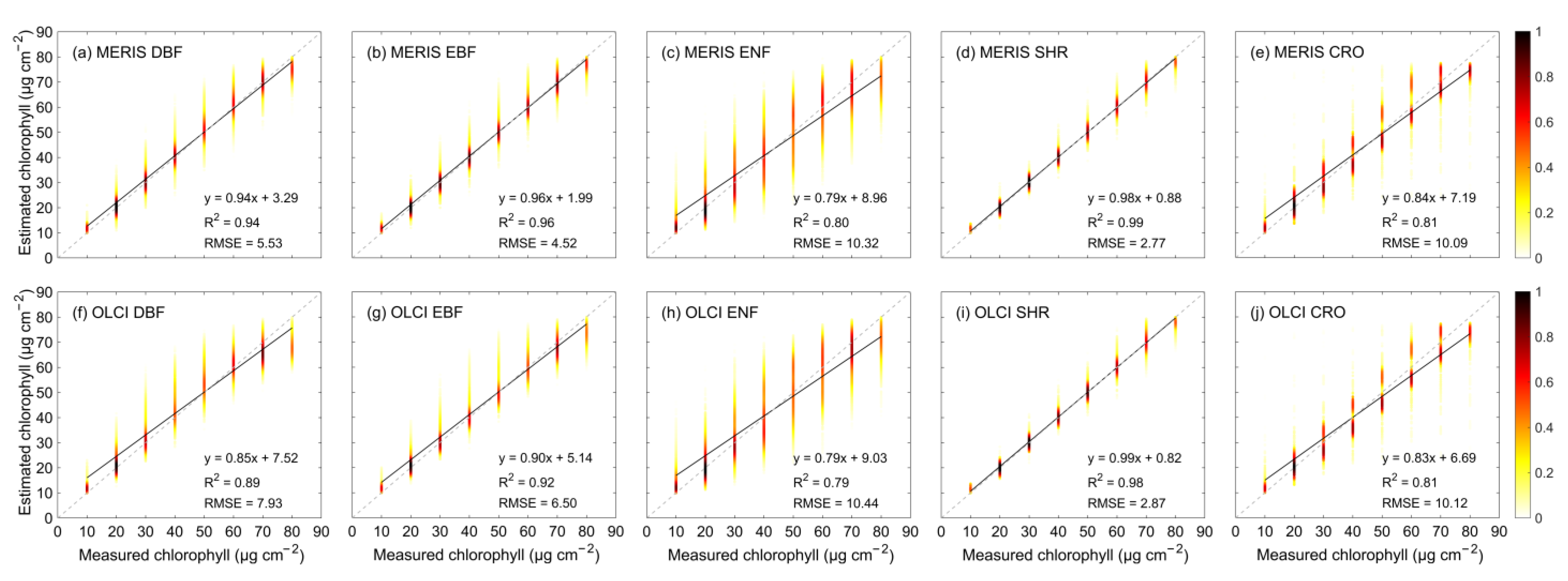
3.1. Validation of LUT Algorithms for LCC Inversion Using the Synthetic Dataset
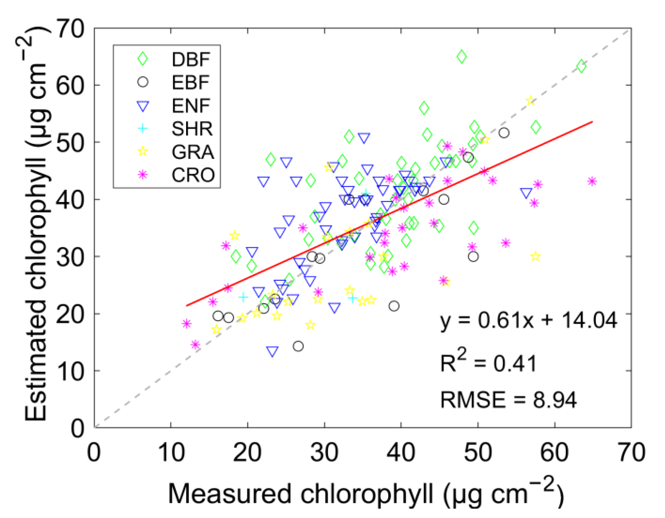
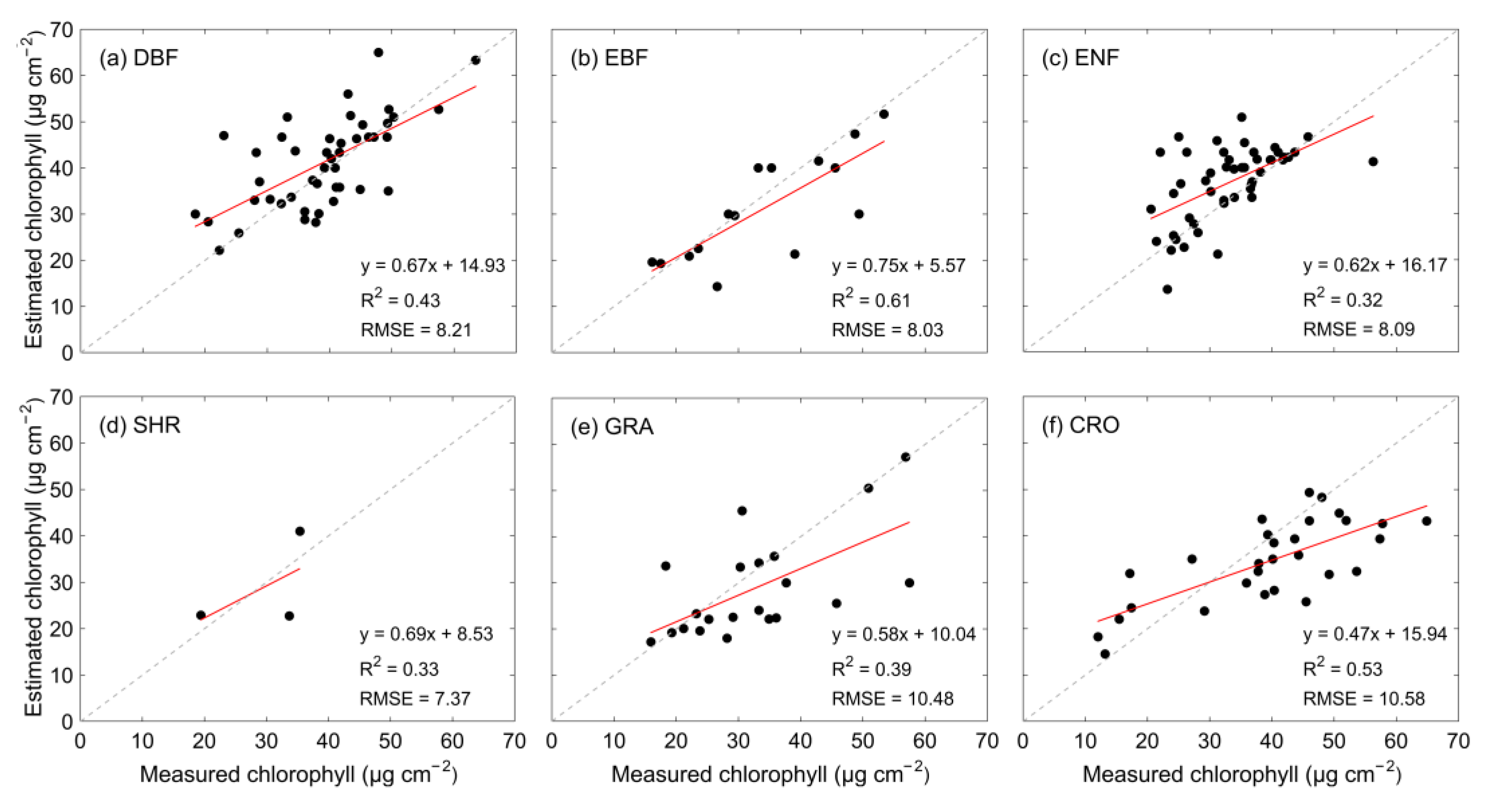
3.2. Validation of the GLCC Dataset Using Field Measurements
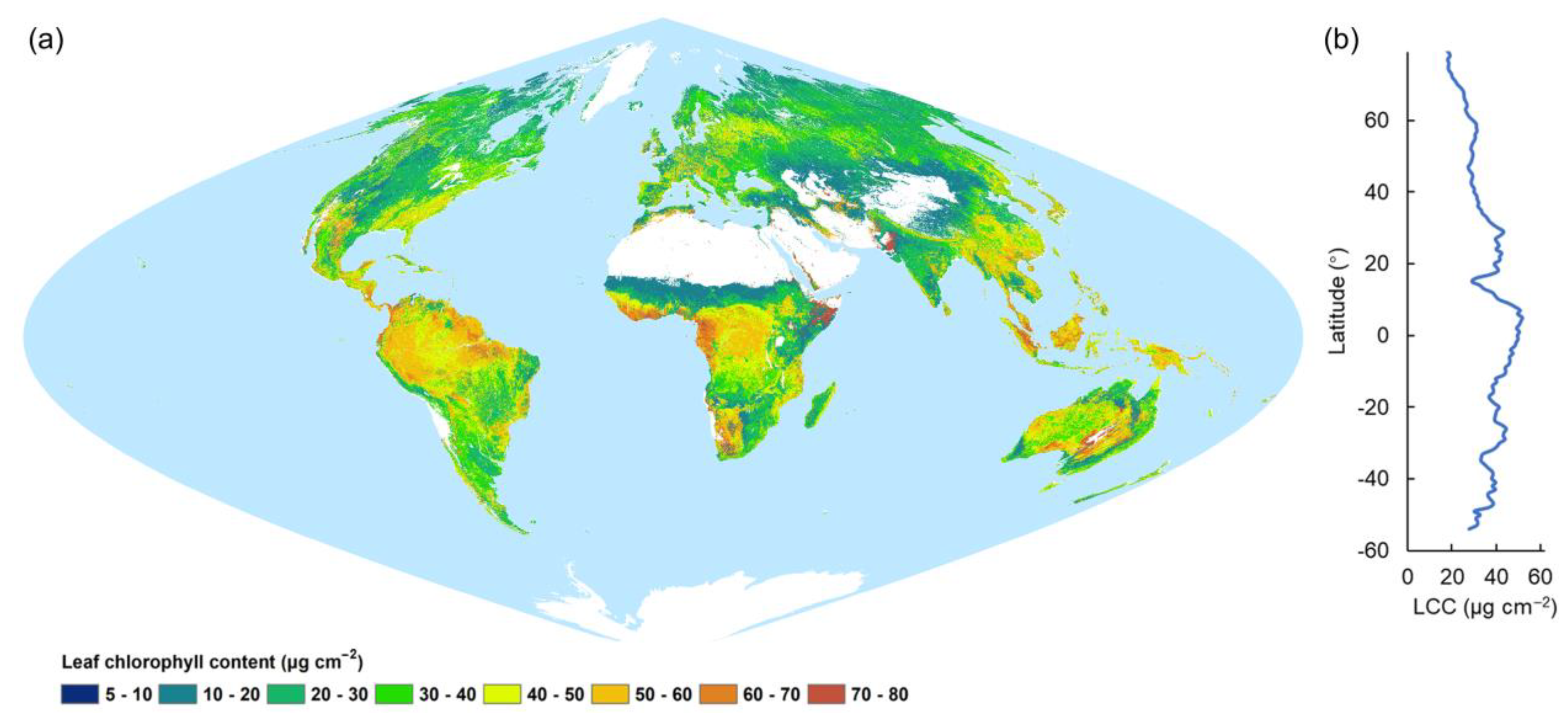
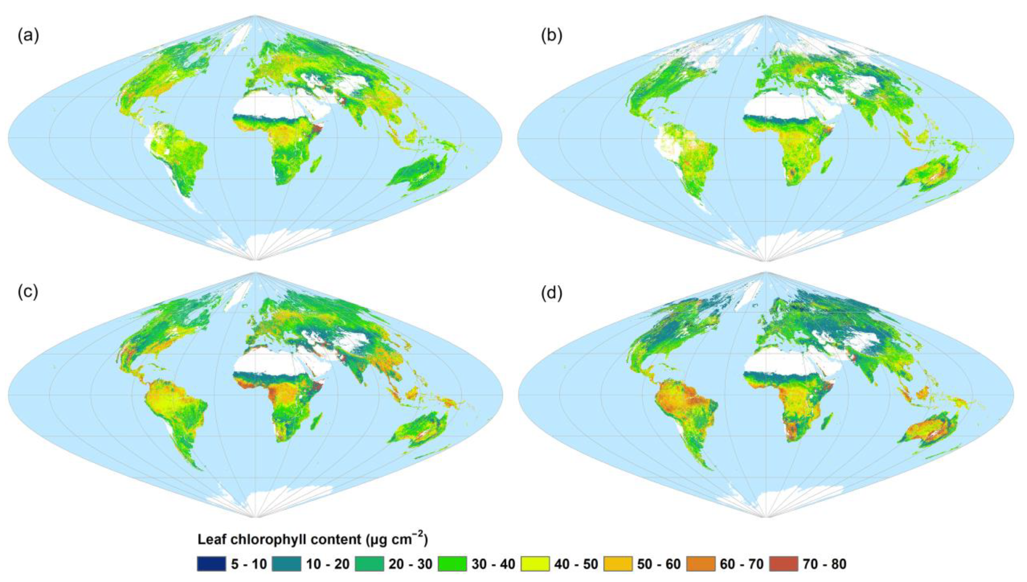
3.3. Spatial and Temporal Trends in Global Leaf Chlorophyll Content
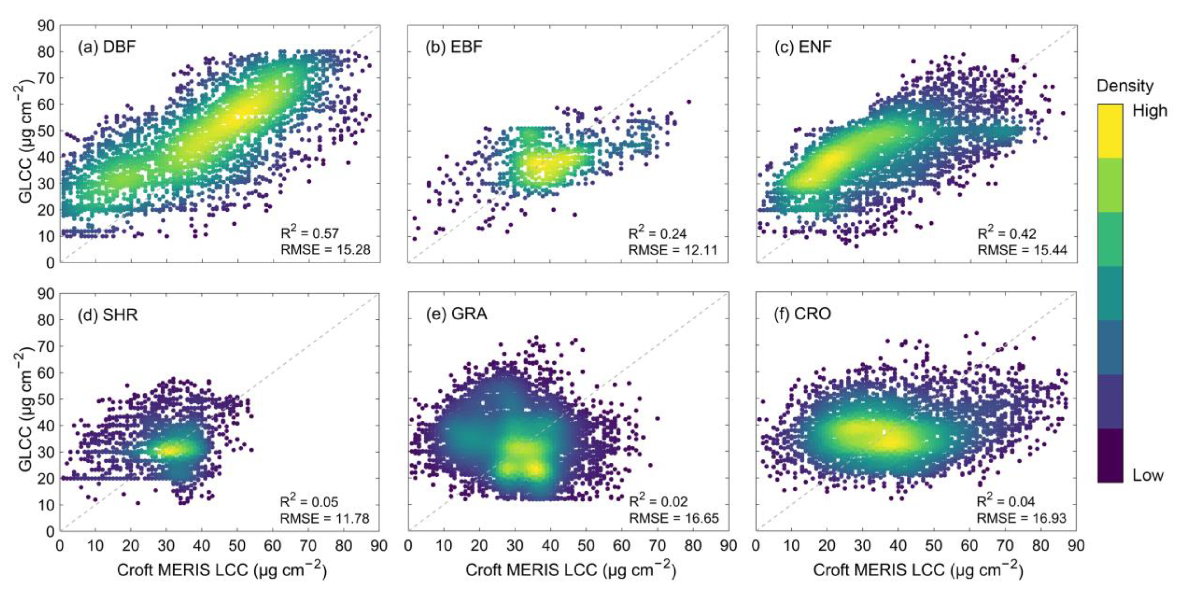
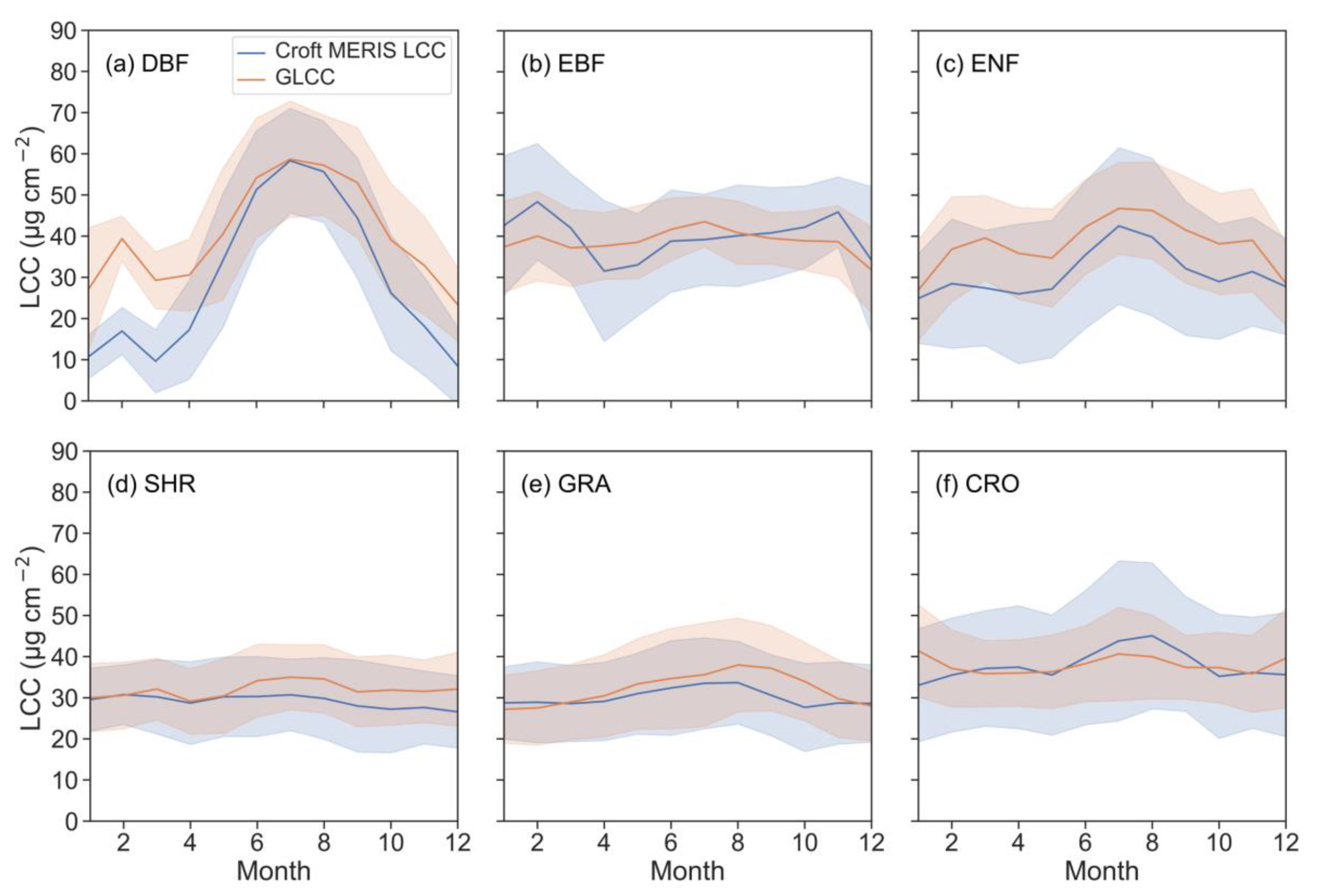
3.4. Comparisons of the GLCC Dataset and Croft MERIS LCC Dataset
4. Discussion
4.1. Advance in the GLCC Dataset
4.2. Uncertainty in the GLCC Dataset
5. Conclusions
Author Contributions
Funding
Institutional Review Board Statement
Informed Consent Statement
Data Availability Statement
Acknowledgments
Conflicts of Interest
References
- Badgley, G.; Field, C.B.; Berry, J.A. Canopy near-infrared reflectance and terrestrial photosynthesis. Sci. Adv. 2017, 3, e1602244. [Google Scholar] [CrossRef] [Green Version]
- Xiao, J.; Chevallier, F.; Gomez, C.; Guanter, L.; Hicke, J.A.; Huete, A.R.; Ichii, K.; Ni, W.; Pang, Y.; Rahman, A.F.; et al. Remote sensing of the terrestrial carbon cycle: A review of advances over 50 years. Remote Sens. Environ. 2019, 233, 111383. [Google Scholar] [CrossRef]
- Ryu, Y.; Berry, J.A.; Baldocchi, D.D. What is global photosynthesis? History, uncertainties and opportunities. Remote Sens. Environ. 2019, 223, 95–114. [Google Scholar] [CrossRef]
- Gitelson, A.; Gritz, Y.; Merzlyak, M.N. Relationships between leaf chlorophyll content and spectral reflectance and algorithms for non-destructive chlorophyll assessment in higher plant leaves. J. Plant Physiol. 2003, 160, 271–282. [Google Scholar] [CrossRef] [PubMed]
- Li, Y.; Ma, Q.; Chen, J.M.; Croft, H.; Luo, X.; Zheng, T.; Rogers, C.; Liu, J. Fine-scale leaf chlorophyll distribution across a deciduous forest through two-step model inversion from Sentinel-2 data. Remote Sens. Environ. 2021, 264, 112618. [Google Scholar] [CrossRef]
- Croft, H.; Chen, J.; Luo, X.; Bartlett, P.; Chen, B.; Staebler, R.M. Leaf chlorophyll content as a proxy for leaf photosynthetic capacity. Glob. Change Biol. 2017, 23, 3513–3524. [Google Scholar] [CrossRef] [PubMed] [Green Version]
- Qian, X.; Liu, L.; Croft, H.; Chen, J.M. Relationship between leaf maximum carboxylation rate and chlorophyll content preserved across 13 species. J. Geophys. Res. Biogeosci. 2021, 126, e2020JG006076. [Google Scholar] [CrossRef]
- Wang, S.; Li, Y.; Ju, W.; Chen, B.; Chen, J.; Croft, H.; Mickler, R.A.; Yang, F. Estimation of leaf photosynthetic capacity from leaf chlorophyll content and leaf age in a subtropical evergreen coniferous plantation. J. Geophys. Res. Biogeosci. 2020, 125, e2019JG005020. [Google Scholar] [CrossRef]
- Lu, X.; Ju, W.; Li, J.; Croft, H.; Chen, J.M.; Luo, Y.; Yu, H.; Hu, H. Maximum carboxylation rate estimation with chlorophyll content as a proxy of rubisco content. J. Geophys. Res. Biogeosci. 2020, 125, e2020JG005748. [Google Scholar] [CrossRef]
- Li, J.; Lu, X.; Ju, W.; Li, J.; Zhu, S.; Zhou, Y. Seasonal changes of leaf chlorophyll content as a proxy of photosynthetic capacity in winter wheat and paddy rice. Ecol. Indic. 2022, 140, 109018. [Google Scholar] [CrossRef]
- Jay, S.; Maupas, F.; Bendoula, R.; Gorretta, N. Retrieving LAI, chlorophyll and nitrogen contents in sugar beet crops from multi-angular optical remote sensing: Comparison of vegetation indices and PROSAIL inversion for field phenotyping. Field Crops Res. 2017, 210, 33–46. [Google Scholar] [CrossRef] [Green Version]
- Kira, O.; Linker, R.; Gitelson, A. Non-destructive estimation of foliar chlorophyll and carotenoid contents: Focus on informative spectral bands. Int. J. Appl. Earth Obs. Geoinf. 2015, 38, 251–260. [Google Scholar] [CrossRef]
- Qian, B.; Ye, H.; Huang, W.; Xie, Q.; Pan, Y.; Xing, N.; Ren, Y.; Guo, A.; Jiao, Q.; Lan, Y. A sentinel-2-based triangular vegetation index for chlorophyll content estimation. Agric. For. Meteorol. 2022, 322, 109000. [Google Scholar] [CrossRef]
- Zhang, Y.; Hui, J.; Qin, Q.; Sun, Y.; Zhang, T.; Sun, H.; Li, M. Transfer-learning-based approach for leaf chlorophyll content estimation of winter wheat from hyperspectral data. Remote Sens. Environ. 2021, 267, 112724. [Google Scholar] [CrossRef]
- Jiang, X.; Zhen, J.; Miao, J.; Zhao, D.; Shen, Z.; Jiang, J.; Gao, C.; Wu, G.; Wang, J. Newly-developed three-band hyperspectral vegetation index for estimating leaf relative chlorophyll content of mangrove under different severities of pest and disease. Ecol. Indic. 2022, 140, 108978. [Google Scholar] [CrossRef]
- Houborg, R.; Anderson, M.C.; Daughtry, C.S.T.; Kustas, W.P.; Rodell, M. Using leaf chlorophyll to parameterize light-use-efficiency within a thermal-based carbon, water and energy exchange model. Remote Sens. Environ. 2011, 115, 1694–1705. [Google Scholar] [CrossRef]
- Luo, X.; Croft, H.; Chen, J.M.; He, L.; Keenan, T.F. Improved estimates of global terrestrial photosynthesis using information on leaf chlorophyll content. Glob. Change Biol. 2019, 25, 2499–2514. [Google Scholar] [CrossRef] [Green Version]
- Piao, S.; Wang, X.; Park, T.; Chen, C.; Lian, X.; He, Y.; Bjerke, J.W.; Chen, A.; Ciais, P.; Tømmervik, H. Characteristics, drivers and feedbacks of global greening. Nat. Rev. Earth Environ. 2020, 1, 14–27. [Google Scholar] [CrossRef] [Green Version]
- Croft, H.; Chen, J.M.; Zhang, Y.; Simic, A. Modelling leaf chlorophyll content in broadleaf and needle leaf canopies from ground, CASI, Landsat TM 5 and MERIS reflectance data. Remote Sens. Environ. 2013, 133, 128–140. [Google Scholar] [CrossRef]
- Darvishzadeh, R.; Skidmore, A.; Abdullah, H.; Cherenet, E.; Ali, A.; Wang, T.; Nieuwenhuis, W.; Heurich, M.; Vrieling, A.; O’Connor, B. Mapping leaf chlorophyll content from Sentinel-2 and RapidEye data in spruce stands using the invertible forest reflectance model. Int. J. Appl. Earth Obs. Geoinf. 2019, 79, 58–70. [Google Scholar] [CrossRef] [Green Version]
- Croft, H.; Chen, J.M.; Wang, R.; Mo, G.; Luo, S.; Luo, X.; He, L.; Gonsamo, A.; Arabian, J.; Zhang, Y. The global distribution of leaf chlorophyll content. Remote Sens. Environ. 2020, 236, 111479. [Google Scholar] [CrossRef]
- Xu, M.; Liu, R.; Chen, J.M.; Shang, R.; Liu, Y.; Qi, L.; Croft, H.; Ju, W.; Zhang, Y.; He, Y. Retrieving global leaf chlorophyll content from MERIS data using a neural network method. ISPRS J. Photogramm. Remote Sens. 2022, 192, 66–82. [Google Scholar] [CrossRef]
- Xu, M.; Liu, R.; Chen, J.M.; Liu, Y.; Wolanin, A.; Croft, H.; He, L.; Shang, R.; Ju, W.; Zhang, Y. A 21-Year Time Series of Global Leaf Chlorophyll Content Maps from MODIS Imagery. IEEE Trans. Geosci. Remote Sens. 2022, 60, 4413513. [Google Scholar] [CrossRef]
- Jay, S.; Gorretta, N.; Morel, J.; Maupas, F.; Bendoula, R.; Rabatel, G.; Dutartre, D.; Comar, A.; Baret, F. Estimating leaf chlorophyll content in sugar beet canopies using millimeter- to centimeter-scale reflectance imagery. Remote Sens. Environ. 2017, 198, 173–186. [Google Scholar] [CrossRef]
- Li, D.; Chen, J.M.; Zhang, X.; Yan, Y.; Zhu, J.; Zheng, H.; Zhou, K.; Yao, X.; Tian, Y.; Zhu, Y. Improved estimation of leaf chlorophyll content of row crops from canopy reflectance spectra through minimizing canopy structural effects and optimizing off-noon observation time. Remote Sens. Environ. 2020, 248, 111985. [Google Scholar] [CrossRef]
- Xu, M.; Liu, R.; Chen, J.M.; Liu, Y.; Shang, R.; Ju, W.; Wu, C.; Huang, W. Retrieving leaf chlorophyll content using a matrix-based vegetation index combination approach. Remote Sens. Environ. 2019, 224, 60–73. [Google Scholar] [CrossRef]
- Houborg, R.; Anderson, M.; Daughtry, C. Utility of an image-based canopy reflectance modeling tool for remote estimation of LAI and leaf chlorophyll content at the field scale. Remote Sens. Environ. 2009, 113, 259–274. [Google Scholar] [CrossRef]
- Zarco-Tejada, P.J.; Berjón, A.; López-Lozano, R.; Miller, J.R.; Martín, P.; Cachorro, V.; González, M.R.; De Frutos, A. Assessing vineyard condition with hyperspectral indices: Leaf and canopy reflectance simulation in a row-structured discontinuous canopy. Remote Sens. Environ. 2005, 99, 271–287. [Google Scholar] [CrossRef]
- Zhang, Y.; Chen, J.M.; Miller, J.R.; Noland, T.L. Leaf chlorophyll content retrieval from airborne hyperspectral remote sensing imagery. Remote Sens. Environ. 2008, 112, 3234–3247. [Google Scholar] [CrossRef]
- Verrelst, J.; Camps-Valls, G.; Muñoz-Marí, J.; Rivera, J.P.; Veroustraete, F.; Clevers, J.G.P.W.; Moreno, J. Optical remote sensing and the retrieval of terrestrial vegetation bio-geophysical properties–A review. ISPRS J. Photogramm. Remote Sens. 2015, 108, 273–290. [Google Scholar] [CrossRef]
- Haboudane, D.; Miller, J.R.; Tremblay, N.; Zarco-Tejada, P.J.; Dextraze, L. Integrated narrow-band vegetation indices for prediction of crop chlorophyll content for application to precision agriculture. Remote Sens. Environ. 2002, 81, 416–426. [Google Scholar] [CrossRef]
- Wu, C.; Niu, Z.; Tang, Q.; Huang, W. Estimating chlorophyll content from hyperspectral vegetation indices: Modeling and validation. Agric. For. Meteorol. 2008, 148, 1230–1241. [Google Scholar] [CrossRef]
- Croft, H.; Chen, J.M.; Zhang, Y. The applicability of empirical vegetation indices for determining leaf chlorophyll content over different leaf and canopy structures. Ecol. Complex. 2014, 17, 119–130. [Google Scholar] [CrossRef]
- Sims, D.A.; Gamon, J.A. Relationships between leaf pigment content and spectral reflectance across a wide range of species, leaf structures and developmental stages. Remote Sens. Environ. 2002, 81, 337–354. [Google Scholar] [CrossRef]
- Daughtry, C.S.T.; Walthall, C.L.; Kim, M.S.; De Colstoun, E.B.; McMurtrey Iii, J.E. Estimating corn leaf chlorophyll concentration from leaf and canopy reflectance. Remote Sens. Environ. 2000, 74, 229–239. [Google Scholar] [CrossRef]
- Yin, G.; Verger, A.; Descals, A.; Filella, I.; Peñuelas, J. A broadband green-red vegetation index for monitoring gross primary production phenology. J. Remote Sens. 2022, 2022, 9764982. [Google Scholar] [CrossRef]
- Croft, H.; Chen, J.M. Leaf pigment content. In Comprehensive Remote Sensing; Elsevier: Amsterdam, The Netherlands, 2017; pp. 117–142. [Google Scholar]
- Sun, J.; Shi, S.; Yang, J.; Du, L.; Gong, W.; Chen, B.; Song, S. Analyzing the performance of PROSPECT model inversion based on different spectral information for leaf biochemical properties retrieval. ISPRS J. Photogramm. Remote Sens. 2018, 135, 74–83. [Google Scholar] [CrossRef]
- Qian, X.; Liu, L. Retrieving crop leaf chlorophyll content using an improved look-up-table approach by combining multiple canopy structures and soil backgrounds. Remote Sens. 2020, 12, 2139. [Google Scholar] [CrossRef]
- Curran, P.J.; Steele, C.M. MERIS: The re-branding of an ocean sensor. Int. J. Remote Sens. 2005, 26, 1781–1798. [Google Scholar] [CrossRef]
- Keller, M.; Schimel, D.S.; Hargrove, W.W.; Hoffman, F.M. A continental strategy for the National Ecological Observatory Network. Ecol. Soc. Am. 2008, 6, 282–284. [Google Scholar] [CrossRef]
- Scholl, V.M.; Cattau, M.E.; Joseph, M.B.; Balch, J.K. Integrating National Ecological Observatory Network (NEON) airborne remote sensing and in-situ data for optimal tree species classification. Remote Sens. 2020, 12, 1414. [Google Scholar] [CrossRef]
- Simic, A.; Chen, J.M.; Noland, T.L. Retrieval of forest chlorophyll content using canopy structure parameters derived from multi-angle data: The measurement concept of combining nadir hyperspectral and off-nadir multispectral data. Int. J. Remote Sens. 2011, 32, 5621–5644. [Google Scholar] [CrossRef]
- Zhang, Y.; Chen, J.M.; Thomas, S.C. Retrieving seasonal variation in chlorophyll content of overstory and understory sugar maple leaves from leaf-level hyperspectral data. Can. J. Remote Sens. 2007, 33, 406–415. [Google Scholar] [CrossRef]
- NEON (National Ecological Observatory Network). Plant Foliar Traits (DP1.10026.001); NEON (National Ecological Observatory Network): Fitchburg, MA, USA, 2022. [Google Scholar] [CrossRef]
- Verhoef, W.; Jia, L.; Xiao, Q.; Su, Z. Unified optical-thermal four-stream radiative transfer theory for homogeneous vegetation canopies. IEEE Trans. Geosci. Remote Sens. 2007, 45, 1808–1822. [Google Scholar] [CrossRef]
- Chen, J.M.; Leblanc, S.G. A four-scale bidirectional reflectance model based on canopy architecture. IEEE Trans. Geosci. Remote Sens. 1997, 35, 1316–1337. [Google Scholar] [CrossRef]
- Féret, J.B.; Gitelson, A.A.; Noble, S.D.; Jacquemoud, S. PROSPECT-D: Towards modeling leaf optical properties through a complete lifecycle. Remote Sens. Environ. 2017, 193, 204–215. [Google Scholar] [CrossRef] [Green Version]
- Chen, J.M.; Leblanc, S.G. Multiple-scattering scheme useful for geometric optical modeling. IEEE Trans. Geosci. Remote Sens. 2001, 39, 1061–1071. [Google Scholar] [CrossRef]
- Sun, Q.; Jiao, Q.; Liu, L.; Liu, X.; Qian, X.; Zhang, X.; Zhang, B. Improving the retrieval of forest canopy chlorophyll content from MERIS dataset by introducing the vegetation clumping Index. IEEE J. Sel. Top. Appl. Earth Obs. Remote Sens. 2021, 14, 5515–5528. [Google Scholar] [CrossRef]
- Chen, J.M.; Menges, C.H.; Leblanc, S.G. Global mapping of foliage clumping index using multi-angular satellite data. Remote Sens. Environ. 2005, 97, 447–457. [Google Scholar] [CrossRef]
- Si, Y.; Schlerf, M.; Zurita-Milla, R.; Skidmore, A.; Wang, T. Mapping spatio-temporal variation of grassland quantity and quality using MERIS data and the PROSAIL model. Remote Sens. Environ. 2012, 121, 415–425. [Google Scholar] [CrossRef]
- Sun, J.; Shi, S.; Wang, L.; Li, H.; Wang, S.; Gong, W.; Tagesson, T. Optimizing LUT-based inversion of leaf chlorophyll from hyperspectral lidar data: Role of cost functions and regulation strategies. Int. J. Appl. Earth Obs. Geoinf. 2021, 105, 102602. [Google Scholar] [CrossRef]
- Gastellu-Etchegorry, J.; Gascon, F.; Esteve, P. An interpolation procedure for generalizing a look-up table inversion method. Remote Sens. Environ. 2003, 87, 55–71. [Google Scholar] [CrossRef]
- Verhoef, W. Light scattering by leaf layers with application to canopy reflectance modeling: The SAIL model. Remote Sens. Environ. 1984, 16, 125–141. [Google Scholar] [CrossRef] [Green Version]
- Atzberger, C. Object-based retrieval of biophysical canopy variables using artificial neural nets and radiative transfer models. Remote Sens. Environ. 2004, 93, 53–67. [Google Scholar] [CrossRef]
- Combal, B.; Baret, F.; Weiss, M.; Trubuil, A.; Mace, D.; Pragnere, A.; Myneni, R.; Knyazikhin, Y.; Wang, L. Retrieval of canopy biophysical variables from bidirectional reflectance—Using prior information to solve the ill-posed inverse problem. Remote Sens. Environ. 2003, 84, 1–15. [Google Scholar] [CrossRef]
- Atzberger, C.; Darvishzadeh, R.; Immitzer, M.; Schlerf, M.; Skidmore, A.; Le Maire, G. Comparative analysis of different retrieval methods for mapping grassland leaf area index using airborne imaging spectroscopy. Int. J. Appl. Earth Obs. Geoinf. 2015, 43, 19–31. [Google Scholar] [CrossRef] [Green Version]
- Zhang, H.; Li, J.; Liu, Q.; Lin, S.; Huete, A.; Liu, L.; Croft, H.; Clevers, J.G.P.W.; Zeng, Y.; Wang, X.; et al. A novel red-edge spectral index for retrieving the leaf chlorophyll content. Methods Ecol. Evol. 2022, 13, 2771–2787. [Google Scholar] [CrossRef]
- Roosjen, P.P.J.; Brede, B.; Suomalainen, J.M.; Bartholomeus, H.M.; Kooistra, L.; Clevers, J.G.P.W. Improved estimation of leaf area index and leaf chlorophyll content of a potato crop using multi-angle spectral data–potential of unmanned aerial vehicle imagery. Int. J. Appl. Earth Obs. Geoinf. 2018, 66, 14–26. [Google Scholar] [CrossRef]
- Atzberger, C.; Darvishzadeh, R.; Schlerf, M.; Le Maire, G. Suitability and adaptation of PROSAIL radiative transfer model for hyperspectral grassland studies. Remote Sens. Lett. 2013, 4, 55–64. [Google Scholar] [CrossRef]
- Darvishzadeh, R.; Matkan, A.A.; Ahangar, A.D. Inversion of a radiative transfer model for estimation of rice canopy chlorophyll content using a lookup-table approach. IEEE J. Sel. Top. Appl. Earth Obs. Remote Sens. 2012, 5, 1222–1230. [Google Scholar] [CrossRef]
- Darvishzadeh, R.; Skidmore, A.; Schlerf, M.; Atzberger, C. Inversion of a radiative transfer model for estimating vegetation LAI and chlorophyll in a heterogeneous grassland. Remote Sens. Environ. 2008, 112, 2592–2604. [Google Scholar] [CrossRef]
- Darvishzadeh, R.; Atzberger, C.; Skidmore, A.; Schlerf, M. Mapping grassland leaf area index with airborne hyperspectral imagery: A comparison study of statistical approaches and inversion of radiative transfer models. ISPRS J. Photogramm. Remote Sens. 2011, 66, 894–906. [Google Scholar] [CrossRef]
- Garrigues, S.; Lacaze, R.; Baret, F.J.T.M.; Morisette, J.T.; Weiss, M.; Nickeson, J.E.; Fernandes, R.; Plummer, S.; Shabanov, N.V.; Myneni, R.B. Validation and intercomparison of global Leaf Area Index products derived from remote sensing data. J. Geophys. Res. Biogeosci. 2008, 113, 2–9. [Google Scholar] [CrossRef]
- Tang, H.; Dubayah, R.; Brolly, M.; Ganguly, S.; Zhang, G. Large-scale retrieval of leaf area index and vertical foliage profile from the spaceborne waveform lidar (GLAS/ICESat). Remote Sens. Environ. 2014, 154, 8–18. [Google Scholar] [CrossRef]
- Zarco-Tejada, P.J.; Hornero, A.; Beck, P.S.A.; Kattenborn, T.; Kempeneers, P.; Hernández-Clemente, R. Chlorophyll content estimation in an open-canopy conifer forest with Sentinel-2A and hyperspectral imagery in the context of forest decline. Remote Sens. Environ. 2019, 223, 320–335. [Google Scholar] [CrossRef] [PubMed]
- Li, D.; Chen, J.M.; Yu, W.; Zheng, H.; Yao, X.; Cao, W.; Wei, D.; Xiao, C.; Zhu, Y.; Cheng, T. Assessing a soil-removed semi-empirical model for estimating leaf chlorophyll content. Remote Sens. Environ. 2022, 282, 113284. [Google Scholar] [CrossRef]
- Reyes-Muñoz, P.; Pipia, L.; Salinero-Delgado, M.; Belda, S.; Berger, K.; Estévez, J.; Morata, M.; Rivera-Caicedo, J.P.; Verrelst, J. Quantifying Fundamental Vegetation Traits over Europe Using the Sentinel-3 OLCI Catalogue in Google Earth Engine. Remote Sens. 2022, 14, 1347. [Google Scholar] [CrossRef] [PubMed]
- Brown, L.A.; Dash, J.; Lidón, A.L.; Lopez-Baeza, E.; Dransfeld, S. Synergetic exploitation of the Sentinel-2 missions for validating the Sentinel-3 ocean and land color instrument terrestrial chlorophyll index over a vineyard dominated mediterranean environment. IEEE J. Sel. Top. Appl. Earth Obs. Remote Sens. 2019, 12, 2244–2251. [Google Scholar] [CrossRef] [Green Version]


| MERIS Channel | Center (nm) | Width (nm) | OLCI Channel | Center (nm) | Width (nm) |
|---|---|---|---|---|---|
| Oa1 | 400 | 15 | |||
| 1 | 412.5 | 10 | Oa2 | 412.5 | 10 |
| 2 | 442.5 | 10 | Oa3 | 442.5 | 10 |
| 3 | 490 | 10 | Oa4 | 490 | 10 |
| 4 | 510 | 10 | Oa5 | 510 | 10 |
| 5 | 560 | 10 | Oa6 | 560 | 10 |
| 6 | 620 | 10 | Oa7 | 620 | 10 |
| 7 | 665 | 10 | Oa8 | 665 | 10 |
| Oa9 | 673.75 | 7.5 | |||
| 8 | 681.25 | 7.5 | Oa10 | 681.25 | 7.5 |
| 9 | 708.75 | 10 | Oa11 | 708.75 | 10 |
| 10 | 753.75 | 7.5 | Oa12 | 753.75 | 7.5 |
| 11 | 760.625 | 3.75 | Oa13 | 761.25 | 2.5 |
| Oa14 | 764.375 | 3.75 | |||
| Oa15 | 767.5 | 2.5 | |||
| 12 | 778.75 | 15 | Oa16 | 778.75 | 15 |
| 13 | 865 | 20 | Oa17 | 865 | 20 |
| 14 | 885 | 10 | Oa18 | 885 | 10 |
| 15 | 900 | 10 | Oa19 | 900 | 10 |
| Oa20 | 940 | 20 | |||
| Oa21 | 1020 | 40 |
| Site Name | Latitude | Longitude | PFT | Dominant Species | Sampling Date | Samples | Reference/Source |
|---|---|---|---|---|---|---|---|
| Sudbury_DBF | 47.16 | −81.71 | DBF | Trembling aspen | Summer 2007 | 2 | Simic, et al. [43] |
| Haliburton | 45.24 | −78.54 | DBF | Sugar maple | May–September 2004 | 8 | Zhang, et al. [44] |
| JERC_DBF | 31.19 | −84.47 | DBF | Southern red oak | September 2019 | 7 | National Ecological Observatory [45] |
| UNDE | 46.23 | −89.54 | DBF | Red and sugar maple, aspen, paper birch | June 2019 | 8 | |
| DELA | 32.54 | −87.81 | DBF | Oak, hickory | April–May 2019 | 4 | |
| CLBJ_DBF | 33.40 | −97.59 | DBF | Post oak, blackjack oak | April–May 2019 | 13 | |
| BONA | 65.16 | −147.54 | DBF | — | July–August 2019 | 3 | |
| SJER_EBF | 37.11 | −119.73 | EBF | Evergreen oak | March–April 2019 | 8 | |
| PUUM | 19.56 | −155.30 | EBF | ‘Ohi’a lehua | January 2019 | 7 | |
| Sudbury_Simic | 47.18 | −81.74 | ENF | Black spruce | Summer 2007 | 5 | Simic, et al. [43] |
| Sudbury_Zhang | 47.16 | −81.74 | ENF | Black spruce | Summer 2003–2004 | 16 | Zhang, et al. [29] |
| JERC_ENF | 31.20 | −84.46 | ENF | Longleaf pine | September 2019 | 9 | National Ecological Observatory [45] |
| NIWO_ENF | 40.04 | −105.56 | ENF | lodgepole pine | August 2019 | 6 | |
| WREF | 45.83 | −121.97 | ENF | Douglas fir, western hemlock, pacific silver fir | July 2019 | 12 | |
| CLBJ_GRA | 33.37 | −97.58 | GRA | Bluestem | April–May 2019 | 6 | |
| NIWO_GRA | 40.05 | −105.58 | GRA | Curly sedge | August 2019 | 3 | |
| SJER_GRA | 37.10 | −119.73 | GRA | Bromus | March–April 2019 | 12 | |
| US-Ne2 | 41.17 | −96.47 | CRO | Soybean | June–September 2004 | 21 | University of Nebraska–Lincoln |
| KONA | 39.13 | −96.63 | CRO | Wheat, corn | July 2019 | 8 | National Ecological Observatory [45] |
| NIWO_SHR | 40.05 | −105.59 | SHR | — | August 2019 | 1 | |
| SJER_SHR | 37.11 | −119.75 | SHR | Manzanita, whitethorn shrub | March–April 2019 | 2 |
| PFT | Min | Max | Mean | SD | CV |
|---|---|---|---|---|---|
| DBF | 18.44 | 63.46 | 38.94 | 9.39 | 0.24 |
| EBF | 16.14 | 53.38 | 34.08 | 11.60 | 0.34 |
| ENF | 20.57 | 56.28 | 33.04 | 7.35 | 0.22 |
| GRA | 15.94 | 57.49 | 32.73 | 11.59 | 0.35 |
| CRO | 12.06 | 64.88 | 39.30 | 13.64 | 0.35 |
| SHR | 19.43 | 35.40 | 29.51 | 7.16 | 0.24 |
| PROSAIL_D | PROSPECT_D+4-Scale | ||||
|---|---|---|---|---|---|
| Parameter | CRO/GRA | DBF | EBF | ENF | SHR |
| Leaf structural parameter (N) | 1.5 | 1.2 | 1.8 | 2.5 | 1.8 |
| Leaf chlorophyll content (LCC, μg cm−2) | 10–80, step 10 | 10–80, step 10 | 10–80, step 10 | 10–80, step 10 | 10–80, step 10 |
| Leaf carotenoid content (Cxc, μg cm−2) | LCC/4 | LCC/7 | LCC/7 | LCC/7 | LCC/7 |
| Equivalent water thickness (Cw, cm) | 0.02 | 0.01 | 0.01 | 0.048 | 0.01 |
| Dry matter content (Cm, g cm−2) | 0.004 | 0.005 | 0.005 | 0.035 | 0.005 |
| Leaf anthocyanin content (Canth, μg cm−2) | 2 | 1 | 1 | 1 | 1 |
| Leaf brown pigment content (Cbp) | 0 | 0 | 0 | 0 | 0 |
| leaf inclination distribution function* | [1,0], [0,−1], [0,1], [−0.35,0.15], [0,0] | — | — | — | — |
| Leaf area index (LAI, m2 m−2) | 0.25, 0.5, 0.75, 1, 1.25, 1.5, 1.75, 2, 3, 4, 5, 6, 7, 8 | 0.5, 1, 2, 4, 6, 8 | 0.5, 1, 2, 4, 6, 8 | 0.5, 1, 2, 4, 6, 8 | 0.5, 1, 2, 4, 6, 8 |
| Hot spot parameter (SL) | 0.05 | — | — | — | — |
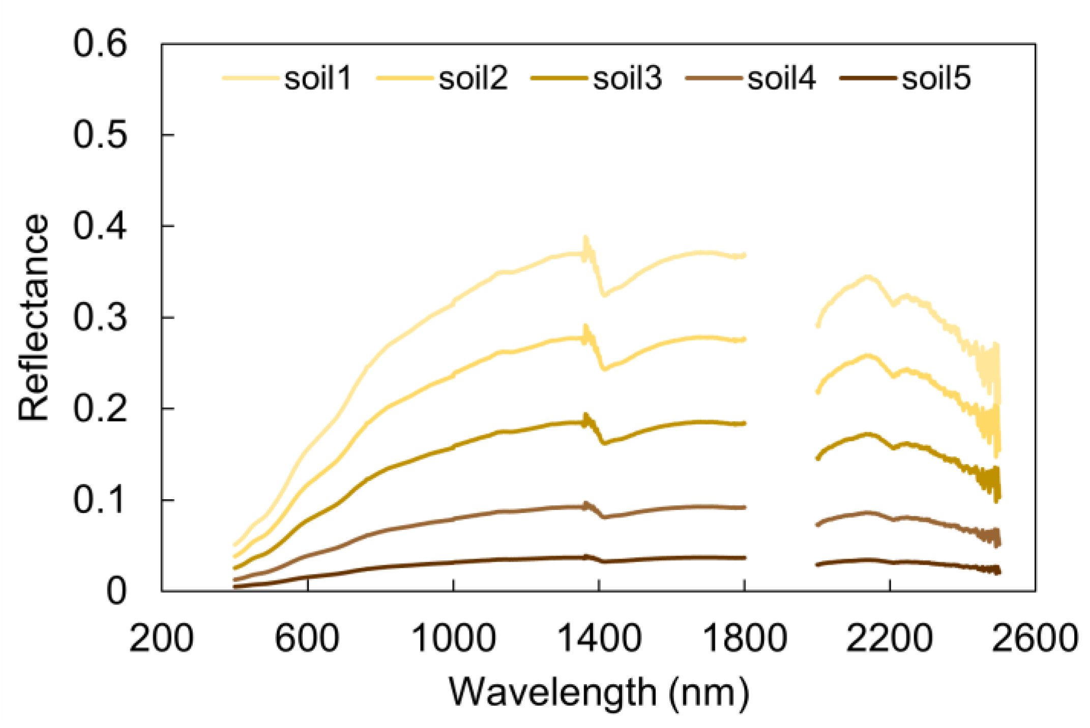
| Soil reflectance (ρs) | As shown in Figure 2 | — | — | — | — |
| Solar zenith angle (θs, °) | 0–60, step 10 | 10–70, step 10 | 10–70, step 10 | 10–70, step 10 | 10–70, step 10 |
| View zenith angle (θv, °) | 0 | 0 | 0 | 0 | 0 |
| Relative azimuth angle (φ, °) | 0 | 0 | 0 | 0 | 0 |
| Stand density (trees/ha) | — | 1000, 2000, 3000, 4000 | 1000, 2000, 3000, 4000 | 1000, 2000, 3000, 4000, 6000, 8000, 12,000 | 1000, 2000, 3000, 4000 |
| Stick height (m) | — | 1, 5, 10 | 1, 5, 10 | 1, 5, 10 | 1, 2, 3 |
| Crown height (m) | — | 5, 10, 20 | 5, 10, 20 | 5, 10, 20 | 1, 2, 3 |
| Crown radius (m) | — | 0.75, 1, 1.25, 1.5 | 0.75, 1, 1.25, 1.5 | 0.5, 0.75, 1, 1.25 | 0.75, 1, 1.25, 1.5 |
| Crown shape | — | Spheroid | Spheroid | Cone & cylinder | Spheroid |
| Clumping index (ΩE) | — | 0.6, 0.9 | 0.6, 0.9 | 0.5, 0.8 | 0.6, 0.9 |
| Neyman grouping | — | 1, 2, 3 | 1, 2, 3 | 1, 2, 3 | 1, 2, 3 |
| Needle to shoot ratio (γE) | — | 1 | 1 | 1.41 | 1 |
| Background composition | — | Green vegetation and soil | Green vegetation and soil | Green vegetation and soil | Dry grasses and soil |
Disclaimer/Publisher’s Note: The statements, opinions and data contained in all publications are solely those of the individual author(s) and contributor(s) and not of MDPI and/or the editor(s). MDPI and/or the editor(s) disclaim responsibility for any injury to people or property resulting from any ideas, methods, instructions or products referred to in the content. |
© 2023 by the authors. Licensee MDPI, Basel, Switzerland. This article is an open access article distributed under the terms and conditions of the Creative Commons Attribution (CC BY) license (https://creativecommons.org/licenses/by/4.0/).
Share and Cite
Qian, X.; Liu, L.; Chen, X.; Zhang, X.; Chen, S.; Sun, Q. Global Leaf Chlorophyll Content Dataset (GLCC) from 2003–2012 to 2018–2020 Derived from MERIS and OLCI Satellite Data: Algorithm and Validation. Remote Sens. 2023, 15, 700. https://doi.org/10.3390/rs15030700
Qian X, Liu L, Chen X, Zhang X, Chen S, Sun Q. Global Leaf Chlorophyll Content Dataset (GLCC) from 2003–2012 to 2018–2020 Derived from MERIS and OLCI Satellite Data: Algorithm and Validation. Remote Sensing. 2023; 15(3):700. https://doi.org/10.3390/rs15030700
Chicago/Turabian StyleQian, Xiaojin, Liangyun Liu, Xidong Chen, Xiao Zhang, Siyuan Chen, and Qi Sun. 2023. "Global Leaf Chlorophyll Content Dataset (GLCC) from 2003–2012 to 2018–2020 Derived from MERIS and OLCI Satellite Data: Algorithm and Validation" Remote Sensing 15, no. 3: 700. https://doi.org/10.3390/rs15030700