Article

A Spectral–Spatial Method for Mapping Fire Severity Using Morphological Attribute Profiles

1
School of Geophysics and Geomatics, China University of Geosciences, Wuhan 430074, China
2
Hubei Subsurface Multi-Scale Imaging Key Laboratory, China University of Geosciences, Wuhan 430074, China
*
Author to whom correspondence should be addressed.
Remote Sens. 2023, 15(3), 699; https://doi.org/10.3390/rs15030699
Submission received: 15 December 2022 / Revised: 20 January 2023 / Accepted: 22 January 2023 / Published: 24 January 2023
(This article belongs to the Section Earth Observation for Emergency Management)

Abstract

:
Fast and accurate fire severity mapping can provide an essential resource for fire management and studying fire-related ecological and climate change. Currently, mainstream fire severity mapping approaches are based only on pixel-wise spectral features. However, the landscape pattern of fire severity originates from variations in spatial dependence, which should be described by spatial features combined with spectral features. In this paper, we propose a morphological attribute profiles-based spectral–spatial approach, named Burn Attribute Profiles (BAP), to improve fire severity classification and mapping accuracy. Specifically, the BAP method uses principal component transformation and attributes with automatically determined thresholds to extract spatial features, which are integrated with spectral features to form spectral–spatial features for fire severity. We systematically tested and compared the BAP-based spectral–spatial features and spectral index features in the extremely randomized trees machine learning framework. Sentinel-2 imagery was used for seven fires in the Mediterranean region, while Landsat-8 imagery was used for another seven fires in the northwestern continental United States region. The results showed that, except for 2 fires (overall accuracy (OA) for EMSR213_P: 59.6%, EL: 59.5%), BAP performed well for the other 12 fires (OA for the 2 fires: 60–70%, 6 fires: 70–80%, 4 fires: >80%). Furthermore, compared with the spectral indices-based method, the BAP method showed OA improvement in all 14 fires (OA improvement in Mediterranean: 0.2–14.3%, US: 4.7–12.9%). Recall and Precision were also improved for each fire severity level in most fire events. Moreover, the BAP method improved the “salt-and-pepper” phenomenon in the homogeneous area, where the results are visually closest to the reference data. The above results suggest that the spectral–spatial method based on morphological attribute profiles can map fire severity more accurately.

1. Introduction

Forest fires are a vital disturbance affecting forest ecosystems [1,2] and are also widely recognized as a significant factor in global carbon emissions [3,4]. Additionally, fires can affect humans in many ways, including property damage, crop loss, infrastructure damage, and life loss [5]. Fire severity, usually defined as the loss or decomposition of organic material above and below ground, including partial or total plant mortality [6], correlates with fire intensity within the plant community. Fire severity can be used to describe fire conditions and as a standardized indicator of environmental changes in post-fire areas [7], which can reflect the succession of plant and animal communities and changes in surface materials. Accurate fire severity mapping helps land managers and researchers to provide practical information on post-fire areas for scientific post-fire ecological restoration [8], fire management strategies, and insight into the effects of fire on biota and ecosystem processes [9]. Currently, fire severity mapping is mainly studied using remote sensing data. The impact of fire on vegetation and soil can be characterized by remote sensing images [10] as changes in the spectral features of ground objects. The bands of near-infrared, short-wave infrared, and thermal infrared are the most sensitive to the intensity of forest fires [11,12,13].
While many methods have been developed to predict and map fire severity using remote sensing imagery, most have focused on remote sensed spectral indices methods [11]. Spectral indices (SI) [14], such as the Normalized Difference Vegetation Index (NDVI) [15] and Normalized Burn Ratio (NBR) [16], are often used to extract spectral features of severity. Epting and Verbyla used Landsat to evaluate the classification performance of many spectral indices for forest fire severity. They tested in four forest fire zones within Alaska using 13 spectral indices in dense coniferous and broadleaf forest environments. They showed that the NBR, which contains near- and mid-infrared bands, had the highest correlation with the Composite Burn Index (CBI) and was most suitable for forest fire severity classification [11]. Escuin and Navarro [17] analyzed the ability of NBR, NDVI, differenced NBR (dNBR), and differenced NDVI (dNDVI) extracted from Landsat imagery for fire severity assessment. They studied three fires in southern Spain and found that dNBR was optimal for discriminating between different fire severities.
More research into the direct estimation of biophysical measures would reduce current overreliance on burn severity indices. Physical-based models, such as Radiative Transfer Models, which take advantage of specific physical reflectance properties of the surface to simulate spectral signatures for vegetation, are appealing approaches for predicting burn severity from satellite imagery [18,19]. Others have estimated severity from post-fire satellite imagery based on spectral mixture analysis [18,20,21], which estimates the fractional cover of biographical variables at the subpixel level.
Another approach is to use machine learning (ML) classifiers to predict the degree of fire severity [22,23,24]. ML classifier methods outperform simple empirical statistical models in handling complex interactions among multiple scenes, scales, and aggregation degrees [25,26]. They can improve the classification accuracy of strongly heterogeneous surface regions commonly occurring in remote sensing [24,27]. Collins et al. [25] investigated the application of random forest (RF) in fire severity classification, evaluated the performance of RF, and demonstrated RF’s great superiority over the traditional single-index empirical model method. Syifa et al. [28] proposed a Support Vector Machine algorithm optimized with an Imperialist Competitive Algorithm for fire severity mapping using Landsat-8 and Sentinel-2 imagery and obtained high classification accuracy.
All of the aforementioned remote sensed spectral indices-based, direct estimation of biophysical measures-based, and ML classifier-based mapping methods are based only on pixel-related spectral features. However, there are limitations to purely spectral features regarding the classification and mapping of fire severity. The classification results show a salt-and-pepper effect, with individual pixels classified differently from their neighbors in homogeneous areas [25,29,30]. The landscape pattern of fire severity originates from variations in spatial dependence, which arise when the value of a pixel recorded at a location is highly related to the values in surrounding locations [18,31,32]. Therefore, the spectral and spatial features, i.e., spectral–spatial features, should be integrated to improve the accuracy of fire severity classification and mapping.
The significant number of contributions in the literature that address the application of the spectral–spatial method to many tasks (e.g., classification [33], segmentation [34], super-resolution mapping [35], etc.) prove how the spectral–spatial method is an effective and modern tool. In recent years, mathematical morphology-based spectral–spatial methods have attracted more attention [33,36]. The Extended Multi-Attribute Profiles method (EMAPs) is one of the main morphological spectral–spatial feature extraction methods [36]. EMAPs is an extension of morphological attribute profiles (APs) [37,38], which filter one base image using attribute filters with different thresholds to obtain multi-scale and multi-level filtering results. The base images can be obtained using dimensionality reduction methods, such as principal component analysis, independent component analysis, and target-constrained interference-minimized band selection [39]. EMAPs was proposed for spatial feature extraction of high-resolution hyperspectral imagery for land cover classification [40]. In addition to land cover and land use, EMAPs has been widely used in other fields. Licciardi et al. used EMAPs and moment of inertia to invert the heights of buildings in Worldview-2 multi-angle images, and the inversion results were closer to the actual data [41]. Falco et al. used EMAPs to extract the geometric features of multi-temporal images and then compared the temporal variations in the study area; the experiments obtained the desired results [42]. It has been proven that EMAPs is an effective spatial feature extraction method that allows the selection of attributes in spatial features flexibly to suit the actual situation [43], and it can also combine spatial features with spectral ones [44], which significantly enriches the decision information for image classification. Although EMAPs has shown better classification results in several domains, its overly flexible scalability makes attribute and threshold selection a critical issue when applied to new domains [45].
This study aims to propose a mathematical morphology-based spectral–spatial method for fire severity mapping. Specifically, we aim to answer the following questions: (1) How effective is the performance of the EMAPs-based spectral–spatial model, named the Burn Attribute Profiles (BAP), for fire severity mapping in different regions with different remote sensed imageries? (2) Is the inclusion of spatial features beneficial for classification (comparing BAP and SI methods)? and (3) Can the BAP method improve the salt-and-pepper phenomenon in homogeneous regions in fire severity mapping results?
The primary contributions of this work can be summarized as follows. To the best of our knowledge, this paper describes the first time the spectral–spatial method has been used for fire severity mapping. We explore the powerful prediction capability of EMAPs-based spectral–spatial features to classify fire severity according to the actual fire situation. Specifically, this study selected two study areas (the Mediterranean region and the northwestern continental United States region), each containing seven fire events. The classification assessment and mapping of the two areas are independent of each other and are not compared with each other. We used different remote sensing imageries (Sentinel-2, Landsat-8) in the two study areas. The two study areas applied different data types to show that the BAP model still has good applicability with different data types. Then, we extracted spatial information from post-fire images using the BAP method with automatically determined thresholds for respective attributes and integrated spatial features with spectral ones. We finally used the extremely randomized trees (ERT) [41] classifier to generate fire severity mapping products. Moreover, the BAP method is compared with the traditional SI-based method, which extracts spectral indices using pre- and post-fire images.
Section 2 first describes the study area and the data collected. The proposed fire severity mapping approach is described in Section 3. Section 4 reports the experiments that validate the performance of the method. Section 5 discusses the experimental results and highlights the proposed method’s merits and limitations. The paper is concluded in Section 6.

2. Study Area and Data Description
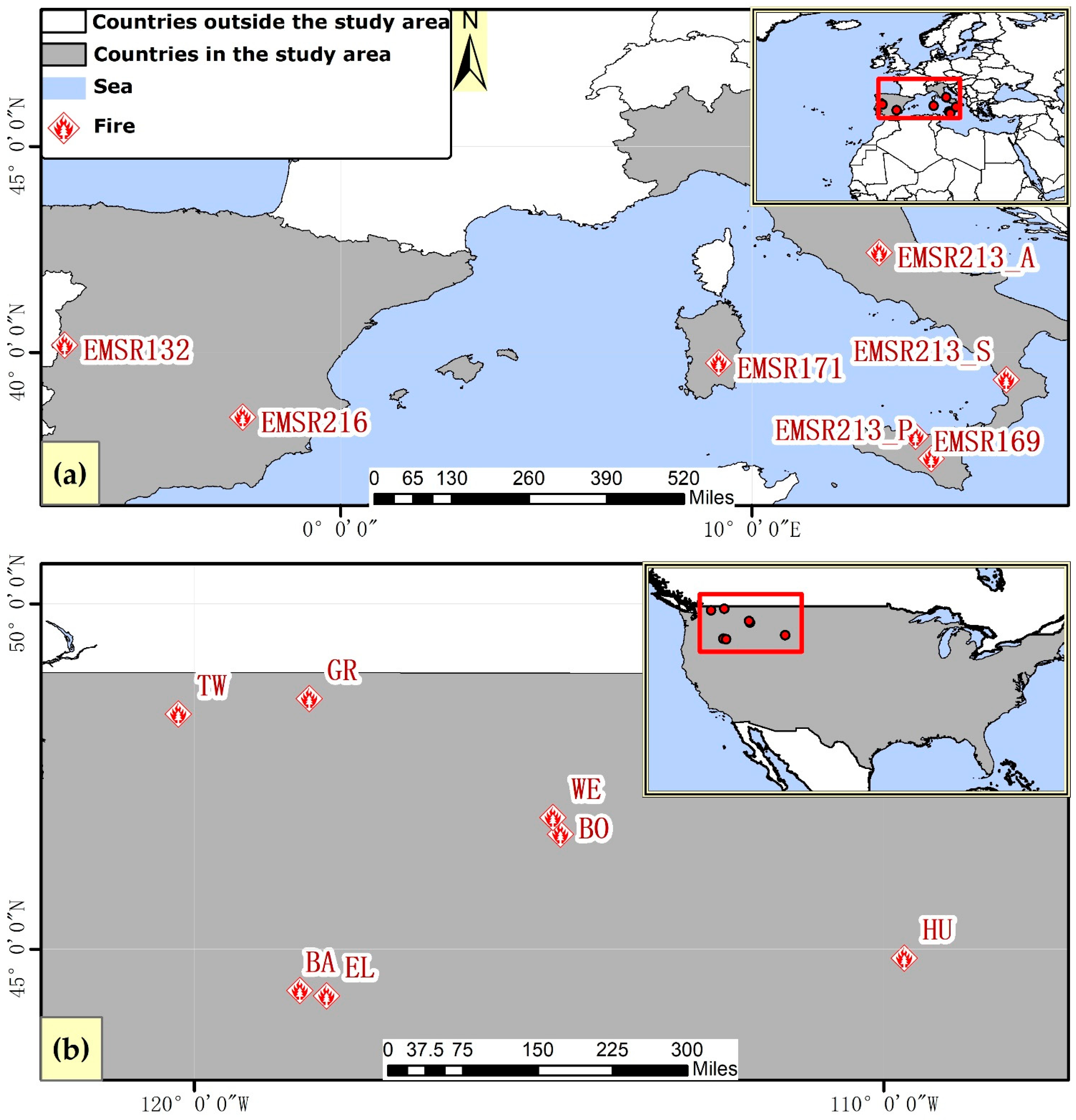
2.1. Study Area

The study area is divided into two large regions: the Mediterranean region of Europe and the northwestern continental United States region (Figure 1). Seven fires are present in each area.
Two of the seven fires in the Mediterranean region are located in Spain, and the other five are in Italy. The fire areas range from 219 to 8178 hectares. Fires are frequent in Spain, with an average of 184 fires per year in the last 15 years (http://effis.jrc.ec.europa.eu/apps/effis.statistics/estimates (accessed on 15 June 2022)) and an average annual fire area of 65,257 hectares. Most of these fires occur between July and September, when the Spanish region is often associated with high temperatures, little rain, and a dry climate, making it highly susceptible to fires. The main land cover types burned in the Spanish region are cropland and woodland, with a combined share of around 80% of monthly average statistics. Of the two fires in Spain, EMSR132 (identified according to the Copernicus Emergency Management Services grading map) burned a vast area of 8178 hectares, including 5482.4 hectares of scrub and woodland (Dominated by Pinus pinaster Ait. and Quercus pyrenaica Wild.); the affected region varies in altitude from 300 to 1400 m, with acidic soils and a climate typical of the Mediterranean. The EMSR216 fire has the smallest size at 219 hectares. The site has a large dense pine forest—approximately 84% forest.
The fires in the Italian region are more frequent than those in Spain. In the past 15 years, an average of 259 fires occurred annually, with an average annual fire area of 47,829 hectares. Italy has an extremely high proportion of farmland within the burn zone, with monthly average statistics exceeding 80%. The five fires in Italy were spread across the Apennines, Sicily, and Sardinia. The EMSR171 fire burned an area of 1632.1 hectares, most of which was artificial plantations, natural grasslands, and woodlands dominated by broadleaf and cork oak forests. Elevation ranges from 380 m to 720 m. According to the 2008 lithological map of Sardinia (http://www.sardegnageoportale.it/ (accessed on 15 June 2022)), the burn area is rich in rock types, including basalt, basaltic andesitic, sandstone, conglomerates, and sandstone. In the east, there are some mica schists and quartzites. The EMSR169 fire, which occurred in Sicily, burned an area of 4057 hectares, with 59% cropland and many olive groves, vineyards, and vegetable gardens. The region has a typical Mediterranean climate with hot, dry summers. Temperatures of 40 degrees Celsius and solid southerly winds exacerbated the wildfires. The remaining three fires were from the same fire record. Still, they were analyzed independently because they were far apart, their land cover types differed significantly, and their extinguishment times varied. The EMSR213_A fire has a total burned area of 890 hectares with undulating terrain, ranging in elevation from 500 m to 1900 m, with approximately 60% forested land and 30% grassland. EMSR213_P has a large area of impact, with a total burned area of 3706.3 hectares, with forest land accounting for about 60% and cropland and shrubs for about 32%. EMSR213_S has a total burned area of 582.1 hectares. The area’s topography is gentle, with elevations ranging from 400 m to 500 m. Cropland accounts for about 60% of the site, and forest land accounts for about 35%.
There are seven fires in the northwestern continental US region, distributed in different states, as shown in Figure 1, where the fires TW and GR are located in Washington State. The area burned by the TW fire is 4558 hectares in total. The burned area is mainly forest and grassland, with apparent zoning. There are large areas of ponderosa pine in the northwestern part of the TW fire area (data on land cover type sourced from the 2011 Native American National Land Cover Database) and extensive grasslands in the central and southeastern parts of the site, with a general topographic relief ranging from 490 to 1337 m in elevation (from NASADEM 30m data). The GR fire covers 3464 hectares, and the study area is located in the northern Rocky Mountains with an altitude of about 1000 m. Most of the interior is covered by dry mesic–montane mixed-conifer forest. Only deciduous shrubs are scattered in the south–central and the northeast. Fires BA and EL are located in Oregon. The BA fire covers 1498 hectares, with a large area of limber–bristlecone pine woodland in the fire area and some grassland and scrub in the southeast. The EL is the largest of all fires at 8483 hectares. Except for its western region, the study area is a basin with a large grassland area. Woodlands are concentrated in the west-facing Rocky Mountains, with large patches of ponderosa pine. Fire WE is located in Montana and has a fire area of 5866 hectares, with multiple woodlands (dry mesic–montane mixed-conifer forest and mesic–montane mixed-conifer forest, among others) in the northern and southern portions of the study area. Fire HU is located in Wyoming and has a burned area of 1498 hectares, with woodland interspersed with grassland within the burn area, ranging in elevation from 2044 m to 2747 m.

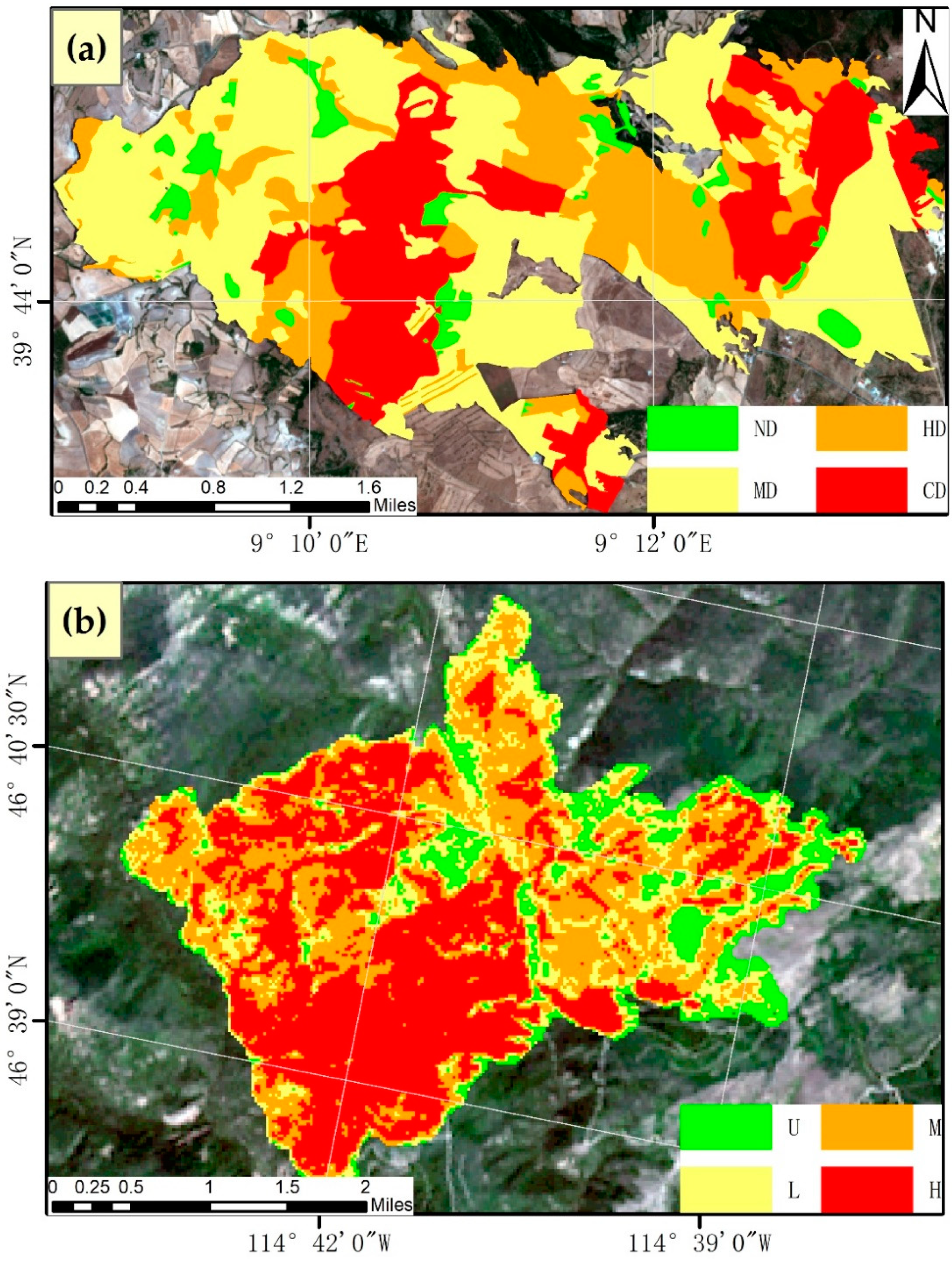
2.2. Fire Severity Data

Fire severity grading maps for use in European wildfire events were obtained from Copernicus Emergency Management Services (CEMS, https://emergency.copernicus.eu (accessed on 21 June 2022)). As part of the EU’s Copernicus program, CEMS uses satellite imagery and other geospatial data to provide free map services when natural disasters, man-made emergencies, and humanitarian crises occur worldwide.
One of CEMS’ services is to provide information on wildfire boundaries, forest fire severity grading maps, and other information used to prevent the loss of life and property and to restore the environment after the fire. The fire severity grading data describe four levels of fire severity: (1) Negligible to Slight Damage (ND); (2) Moderately Damaged (MD); (3) Highly Damaged (HD); (4) Completely Destroyed (CD). The forest fire severity products have been visually interpreted with high-resolution imagery (Pléiades-1A, WorldView-2, etc.) and field-validated, with the overall accuracy of products exceeding 85%. Figure 2a shows the distribution of fire severity reference grading for EMSR171.
Forest fire severity grading maps for use in the continental United States were obtained from the Monitoring Trends in Burn Severity (MTBS, https://www.mtbs.gov/ (accessed on 22 June 2022)) project. The MTBS project was jointly implemented by the United States Geological Survey Center for Earth Resources Observation and Science (EROS) and the USDA Forest Service Geospatial Technology and Applications Center (GTAC) to map fire severity and burn extent for all land in the United States from 1984 to the present, recording fires with areas of 1000 acres and larger in the western United States and those with areas of 500 acres and larger in the eastern United States. The project covers the continental United States, Alaska, Hawaii, and Puerto Rico. The data used in this study uniformly contain the following four classes of forest fire severity: (1) Unburned to Low (U); (2) Low (L); (3) Moderate (M); (4) High (H). Trained image analysts create severity maps based on experience and interpretation of dNBR and RdNBR (Relativized Differenced Normalized Burn Ratio) with manually selected selection thresholds. In this study, we used dNBR offsets to adjust the value of each pixel according to the recommendations of [46] and, thus, obtained a more accurate severity map. Figure 2b shows the distribution of the fire severity reference grading of the BO fire.
It is worth noting that the European CEMS system is more concerned with tree canopy and biomass depletion. In contrast, the US MTBS system focuses on a broader range of criteria while dividing trees, shrubs, grasses, and soils. In the CEMS system, ND stands for unburnt surface with green canopy or burnt surface with unburnt canopy, usually representing 0~10% canopy and reverse burn; MD stands for partial canopy scorch, usually 10–90% canopy score; HD stands for full canopy scorch (±partial canopy consumption), which generally means >90% canopy scorched and <50% canopy biomass consumed; and the CD class represents full canopy consumption, which usually means >50% canopy biomass consumption. For the MTBS system, Unburned to Low represents unburned areas and areas that recover quickly after the fire, such as grasslands, lightly burned surfaces, etc.; Low represents low vegetation (<1 m) and shrubs or trees (1–5 m) that may show significant above-ground scorching. Vegetation density or cover may change significantly, woody debris and newly exposed mineral soils typically exhibit some variability, and canopy tree mortality generally is around 25%. Moderate includes areas that show a uniform transition within low and high burn severity levels. High represents cases where vegetation is almost completely consumed, mostly ash and charcoal remain, and mortality in canopy trees is usually over 75%.

2.3. Remote Sensing Data
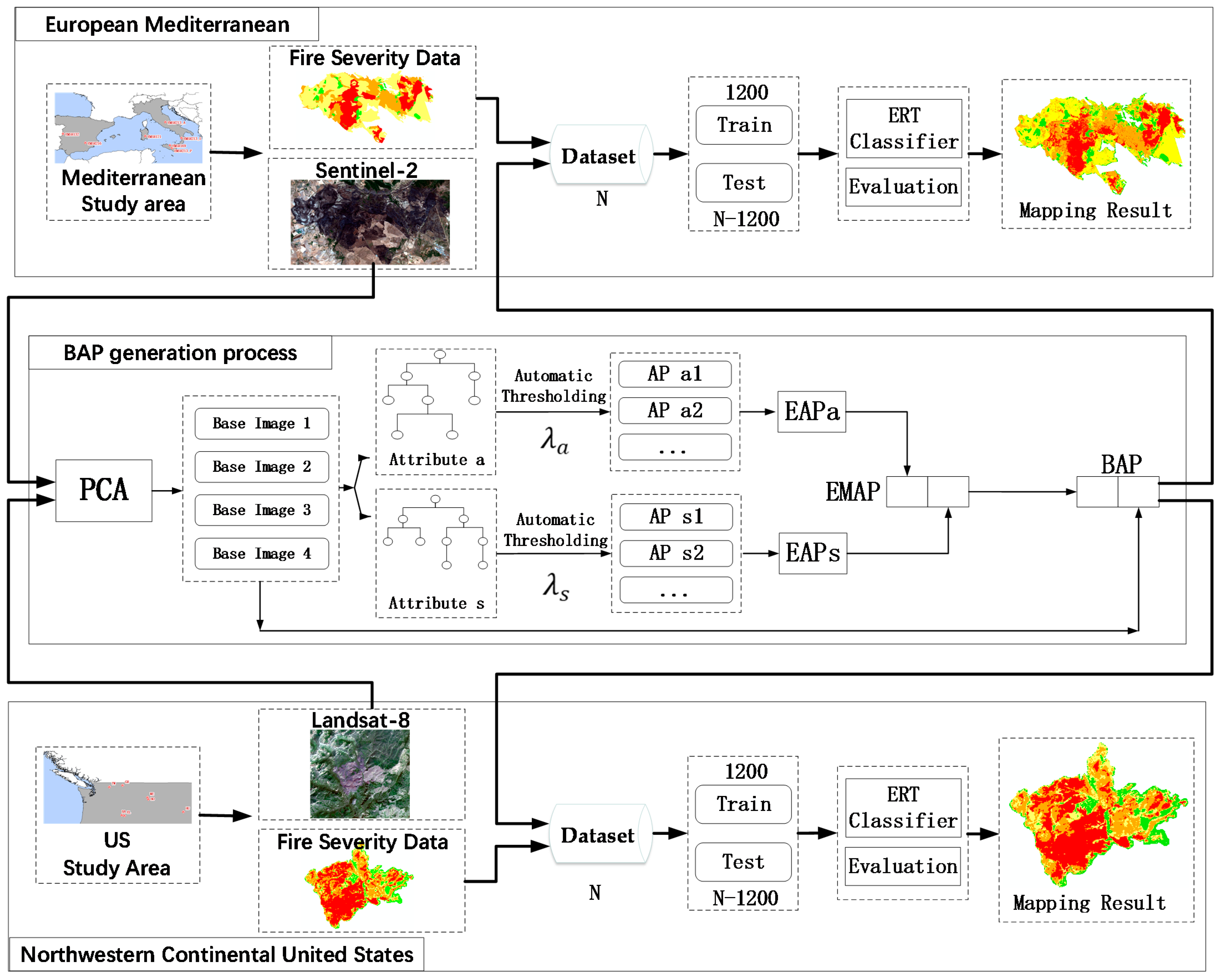
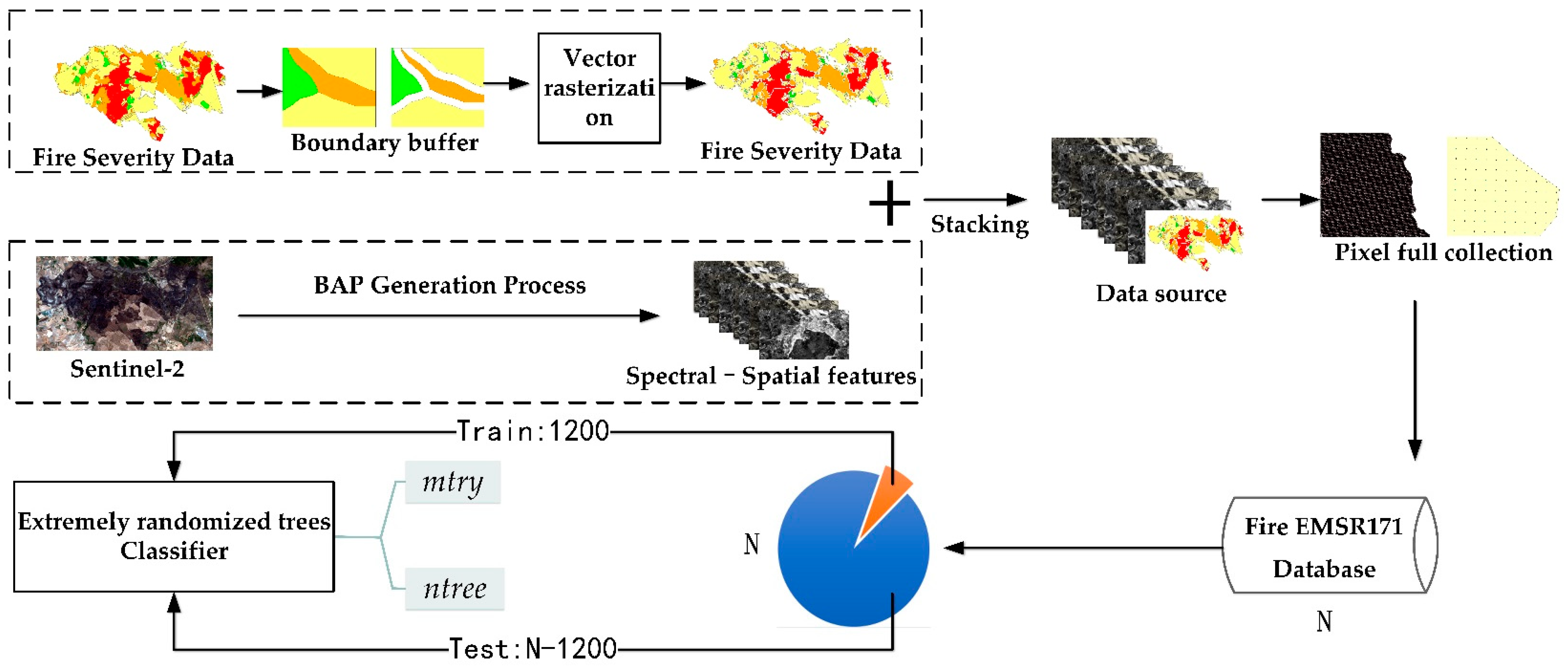
In this paper, two types of remote sensing images (Sentinel-2 and Landsat-8) were used and applied to the corresponding study areas. Sentinel-2 and Landsat-8 provide high-resolution remotely sensed images that can be obtained free of charge and have been used frequently in previous fire severity studies. Specifically, Sentinel-2 images are often used in recent studies because they contain red-edge bands that can describe chlorophyll content and can be used to monitor the health of vegetation.
Sentinel-2 images were used for fire severity mapping in the Mediterranean region of Europe. The BAP method proposed uses only post-fire images as original data, and the acquisition time of post-fire images is shown in Table 1. The start and end times of the European fires are taken from the official document provided by Copernicus (layered
Geospatial document). For the Sentinel-2 data, since some of the fires (e.g., EMSR132) occurred earlier than the production time of the surface reflectivity images (Class 2A products), we selected the top-of-atmosphere reflectivity products (1C products) as the raw images and used the 6S (Second Simulation of the Satellite Signal in the Solar Spectrum) model (https://github.com/samsammurphy/gee-atmcorr-S2 (accessed on 2 July 2022)) for atmospheric correction. Sentinel-2 imagery has multispectral bands with resolutions of 10, 20, and 60 m. In this study, only 10 and 20 m imageries were used, and 20 m imageries were upsampled (interpolated using bilinear interpolation) to 10 m ones. Then, all imageries were combined into one image as the input of the BAP model. The selection of fire images should consider the seasonal discrepancy between the fire environment and the post-fire environment [25]. In this paper, the acquisition time of the European post-fire remote sensing images is no greater than 70 days from the end of the fire, and images taken as close to the fire time as possible are selected. Cloudy conditions in the burn area were also considered when selecting the post-fire remote sensing images, and cloud-free images were selected whenever possible.
Landsat-8 images were used for the fires in the northwestern continental United States region. The acquisition times for post-fire imagery are shown in Table 1, and the fire start times are from the official file, whereas the post-fire imagery was acquired by viewing and comparing the traces in Landsat and related imagery ourselves due to the lack of fire end times in the official file. For the Landsat-8 images, we selected the surface reflectance products and used all seven 30 m resolution bands as the original images for BAP. The post-fire images of Landsat-8 were also selected considering the seasonal differences within the fire environment; post-fire image times similar to those used for the actual severity products and cloud-free images were selected as much as possible.
The remote sensing data used in the study were all sourced from the Google Earth Engine (GEE) platform. The corresponding atmospheric corrections, cropping, and other pre-processing methodologies were also performed in GEE. GEE is a free cloud computing platform that allows for online visualization and computational analysis of large amounts of global-scale geoscience data (especially satellite data). GEE also has an extensive publicly available geospatial database that includes optical and non-optical imagery from various satellite and aerial imaging systems, as well as a variety of other data.

3. Methodology

The graphical overview of the article is shown in Figure 3, which demonstrates the process of classification and mapping using the BAP method for the two study areas in the paper, which can be divided into the following three main processes: (1) using the BAP method to obtain the spatial–spectral features of remote sensing images in the study areas; (2) obtaining the training and test sets from the spatial–spectral feature images and the reference data; (3) using the ERT classifier for classification and mapping of fire severity.

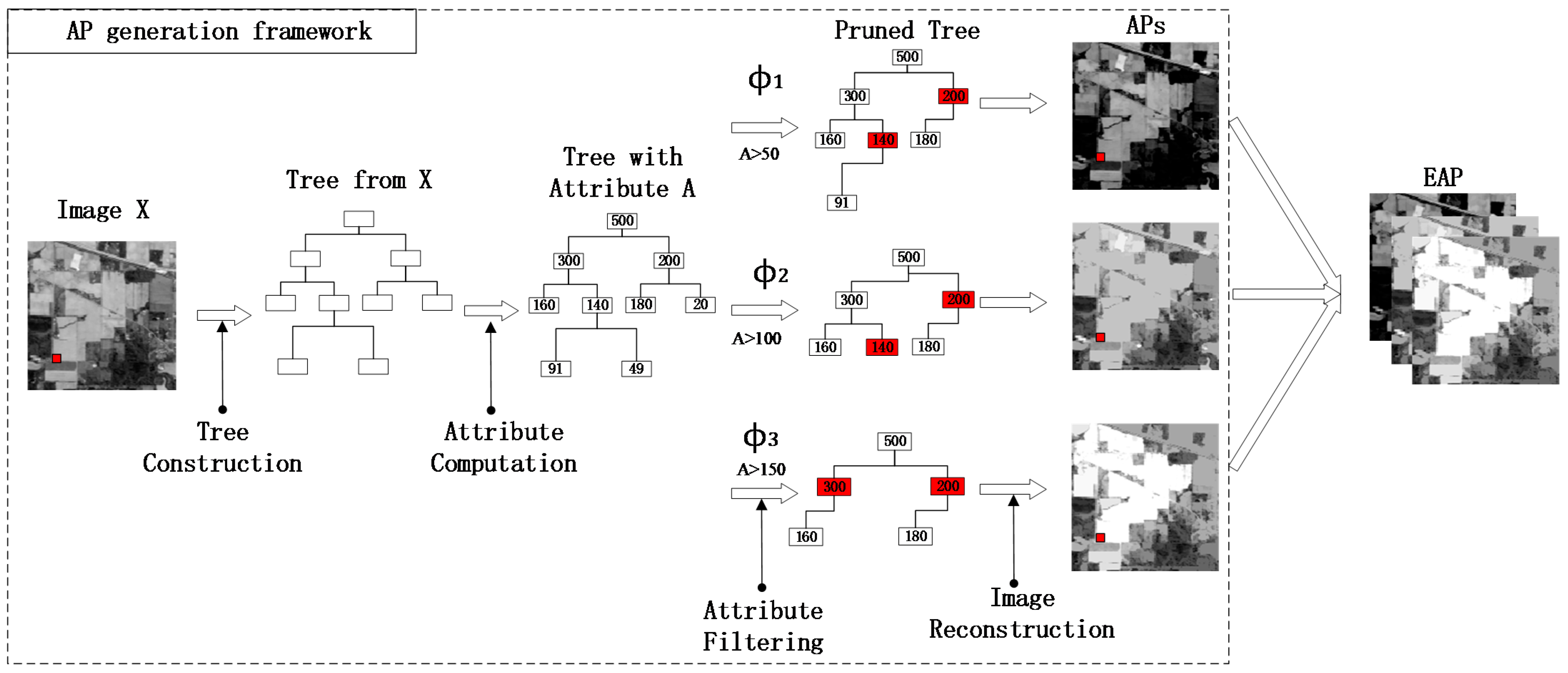
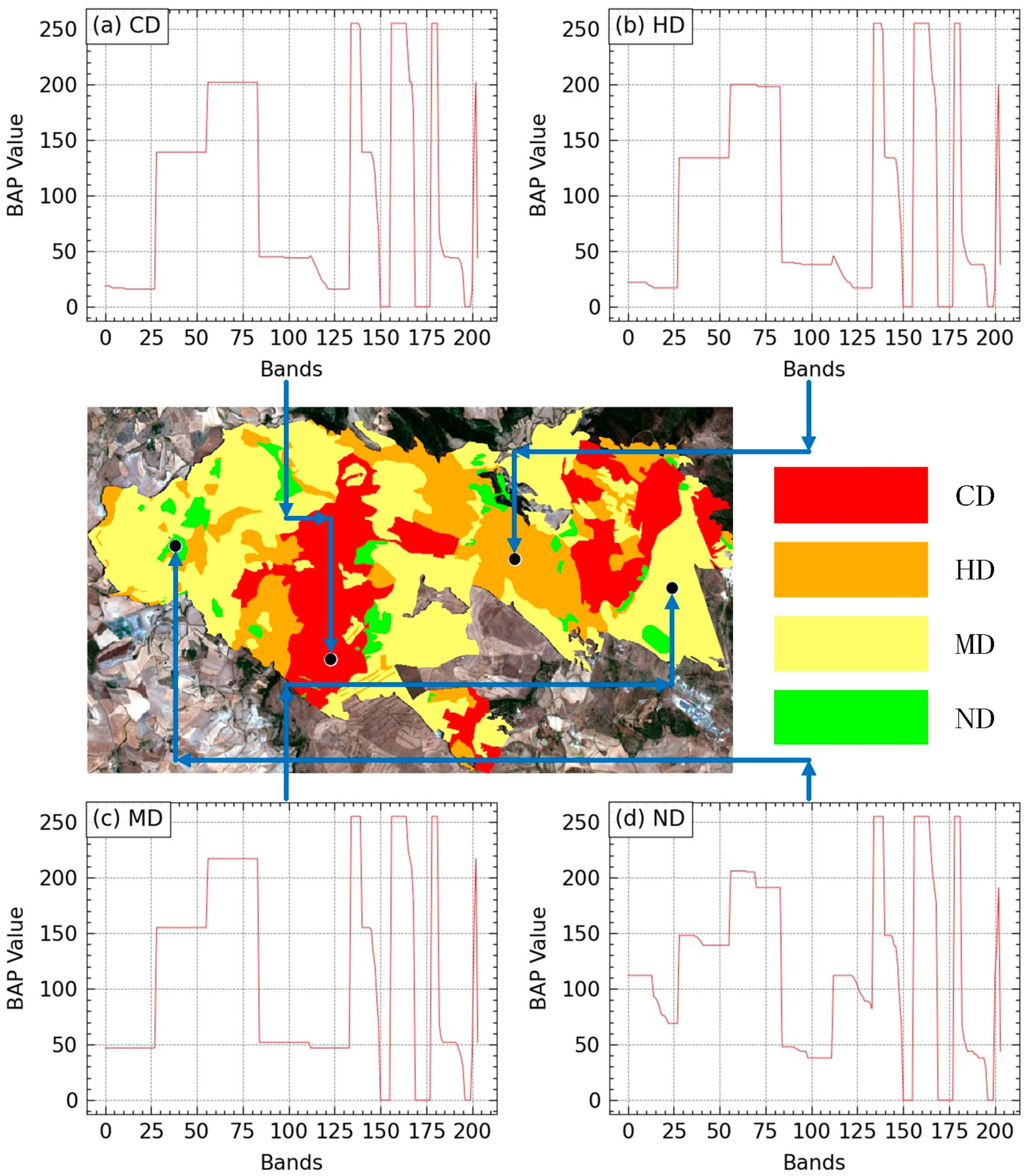
3.1. Burn Attribute Profiles

This paper proposes the BAP method for fire severity feature extraction. BAP is based on the Extended Multi-Attribute Profiles (EMAPs) proposed by Dalla Mura et al. [37,40] and is adapted to the actual situation of the fire.
EMAPs is an extension of the morphological attribute profiles (APs) algorithm. As shown in Figure 4, the process of generating APs can be divided into the following four steps: (1) constructing a tree from grayscale images; (2) calculating the attributes of each node on the tree; (3) filtering (retaining or merging) the attributes of the nodes according to a predefined threshold; (4) reconstructing the image based on the filtered tree to obtain the APs under a certain threshold of attributes. APs provide a multiscale description of an image by applying a series of morphological attribute filters (AFs) based on the max tree (i.e., refinement operation, γ ) and the min tree (i.e., coarsening operation, ϕ ). Unlike image filtering operations that are usually performed directly at the pixel level, AFs operate on each concatenated component. For a grayscale image X, given a series of ordered thresholds { λ 1 , λ 2 , , λ n } , the APs can be expressed as:
APs ( X ) = { ϕ λ n ( X ) , , ϕ λ 1 ( X ) , γ λ 1 ( X ) γ λ n ( X ) }  
where ϕ and γ represent the refinement operation and coarsening one, respectively.
The above is the process for single-band images. For multi-band images, if fewer bands exist, APs can be acquired directly on each band. However, feature extraction is needed to obtain the base image if the input data have more bands. The principal component analysis (PCA) method is commonly used, retaining the first few principal components containing most of the information and then performing morphological attribute profile operations on each principal component to obtain APs. The extended attribute profiles (EAPs) are obtained by superimposing APs of different base images for one attribute, and the EAPs are defined as shown in Equation (2) below:
EAPs ( X ) = { AP ( X 1 ) , AP ( X 2 ) , , AP ( X m ) }
EMAPs are EAPs of multiple attributes for direct stacking, which can extract feature vectors from multiple aspects and describe the fire area’s complex feature characteristics more comprehensively. Specifically, EAPs are stacks of different thresholds for a single attribute, while EMAPs are stacks of different thresholds for multiple attributes. EMAPs can be expressed as follows:
EMAPs ( X ) = { EAPs a 1 ( X 1 ) , EAPs a 2 ( X 2 ) , , EAPs a m ( X m ) }  
EMAPs are very flexible regarding the choice of attributes and can use any defined attribute to measure the connectivity component. For example, they can include attributes related to the region’s shape, such as area, external moments, and moments of inertia, and attributes related to grayscale variation, such as grayscale mean, entropy, and standard deviation.
In this study, we proposed a BAP feature extraction method for fire severity classification by improving EMAPs. Specifically, we improved the EMAPs generation process by adapting three important processes to fire severity classification: (1) base image extraction method, (2) attribute selection, and (3) threshold selection for attributes.
Firstly, to extract base images, we tested three methods: (1) PCA; (2) fast independent component analysis (Fast-ICA); and (3) Joint approximation diagonalization of eigenmatrices ICA (JADE-ICA). These three methods have been used in several studies to extract base images [47,48]. In this study, we tested these three methods’ base image extraction capabilities in seven fires within the European region. The testing results proved that PCA and JADE-ICA performed the best (Table S1 in the supplementary material), and both had advantages and disadvantages in different fire situations. Still, in general, the classification accuracy was similar. In the subsequent experiments of this paper, PCA is used consistently to obtain the base images to ensure uniformity. We retained the first four principal components (PCs), which explained most of the variance in the considered dataset. We retained the four principal component images as features of the spectral information in the BAP method.
Secondly, four common attributes were considered: (1) area of the region (“a”); (2) diagonal of the box bounding the region (“d”); (3) moments of inertia (“i”); and (4) standard deviation of the grayscale values of the pixels in the regions (“s”). We tested the permutations of the four common attributes. We found that the best classification combination was often a combination of all four attributes (“a-i-d-s”) (Table S2 in the supplementary material). Still, the difference in classification accuracy between the combinations of “a-s” and “a-i-d-s” was smaller, while the operation time of “a, s” was much shorter than that of “a-i-d-s”. We can automatically adjust the threshold values of “a” and “s” according to the post-fire image, which is more practical for actual work. Considering all of this, the combination of “a-s” attributes was finally chosen to extract the spatial features of fire severity. These two attributes are clearly correlated with the object level in the image, where “a” can be used to extract information about the object’s scale, and “s” is related to the uniformity of the pixel intensity values.
Finally, for selecting the thresholds of attributes “a” and “s”, we obtained them automatically based on the resolution of the post-fire image and the mean value of the base image’s pixel values, respectively. The threshold selection formula for “a” is as follows:
λ a ( X ) = 1000 ρ { a m i n , a m i n + δ a ,   a m i n + 2 δ a , , a m a x }  
where ρ is the spatial resolution of the image. In this paper, the values of a m i n , a m a x , and δ a were taken as 1, 14, and 1, respectively.
The threshold selection formula for “s” is as follows:
λ s ( X ) = μ i 100 { σ m i n , σ m i n + δ s ,   σ m i n + 2 δ s , , σ m a x }  
where μ i is the mean value of the i-th feature (base image). In this paper, the values of σ m i n , σ m a x , and δ s were taken as 2.5%, 27.5%, and 2.5%, respectively.
In summary, the specific process of the BAP method shown as the “BAP generation process” in Figure 3 contains three parts. Firstly, the PCA method is used to reduce the dimensionality of the pre-processed multispectral images to obtain four base images. Secondly, attributes “a” and “s” are selected to form EMAPs for each base image. Finally, the automatic threshold-selecting method is used in APs for each selected attribute. Specifically, the BAP method extracts a 204-dimension feature image containing 112 feature bands for attribute “a”, 88 feature bands for attribute “s”, and four principal components of the spectral bands. Figure 5 shows the BAP feature curves for the four severity classes within the EMSR171 fire. The code for calculating APs was obtained from [37].

3.2. Extremely Randomized Trees Classification

This paper uses the extremely randomized trees (ERT) model for classification. Similar to the random forest (RF) algorithm, the ERT model is a decision tree-based ensemble classifier that uses a classical top–down process to construct a decision tree. However, unlike RF, it partitions the nodes of the decision tree with completely randomly selected cut points and uses a bootstrap resampling strategy to grow the tree, using the entire learning sample to minimize bias. These strategies allow the algorithm to improve computational efficiency compared to RF while better reducing bias and variance in the model [49]. The basic process of growing an extremely randomized tree can be divided into the following parts: (1) for a given tree node, randomly select a subset of predictor variables from the set of all predictor variables; (2) for each predictor variable in the subset, pick a random cut point ac if the stopping segmentation condition is not satisfied; (3) for the set of all segments derived from the random cut point ac, use the scoring function to score (usually the score is calculated based on information gain) and obtain the set of segments with the largest score; (4) in the next node, a different set of variables is randomly selected from all the predictor variables, then steps (1)~(3) are repeated. When all extremely randomized trees are generated, the predictions of the tree are aggregated by majority voting to arrive at the final prediction. The effectiveness of the ERT classifier has been demonstrated in several studies [50,51]. The ERT classifier parameters are the same as those belonging to RF, focusing on the parameters mtry (a randomly selected subset of model predictor variables) and ntree (the number of decision trees). The implementation of the ERT classifier in the study was obtained from sklearn (https://scikit-learn.org/ (accessed on 5 July 2022)).
Figure 6 shows the collection process for the total dataset from which the training and test sets for the ERT classifier classification need to be sampled. The data sources for total dataset acquisition are the spectral–spatial feature images obtained by the BAP method in the previous section. After obtaining the spatial vector maps of fire severity levels for all fires from CEMS, boundary buffering was applied to them. The data acquired by MTBS are raster images, and we have further made internal buffers after converting the raster images to vectors. We set different buffer distances according to the image cell sizes of different images. Finally, we set the buffer distance to 15 m for Sentinel-2 images and 43 m for Landsat-8 images, which roughly corresponds to the hypotenuse length of each pixel in Sentinel-2 and Landsat-8. Applying an internal buffer to each class of polygon of the fire can prevent sampling points from falling on the boundary between two classes and can also prevent interference between different classes. After that, all pixels within this vector region of the feature image are acquired, and all data are acquired at the center of the pixel. This avoids a single pixel being acquired multiple times and ensures spatial heterogeneity. Each fire in the experiment was collected separately, so each fire had a separate dataset. For subsequent evaluation experiments, each sampling from the dataset is equivalent to sampling from the entire image, which avoids limiting the sample to a certain area and allows the data to be fully utilized.
The acquisition of data points in the total dataset is shown in Table 1, which shows that the amount of data in each fire severity class is unbalanced. Still, the data of each class are sufficient for sampling in the subsequent experiments.

3.3. Experimental Setup
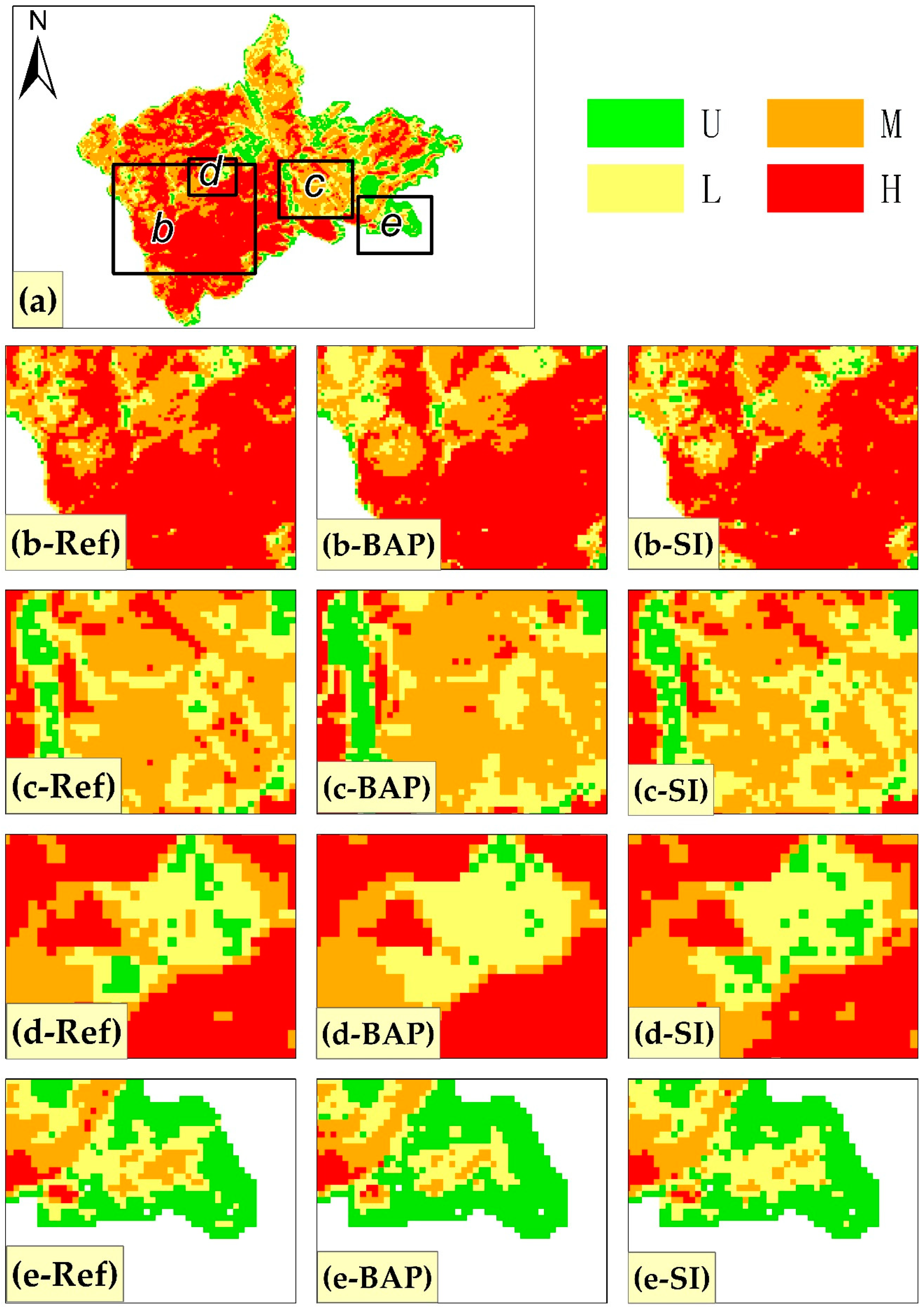
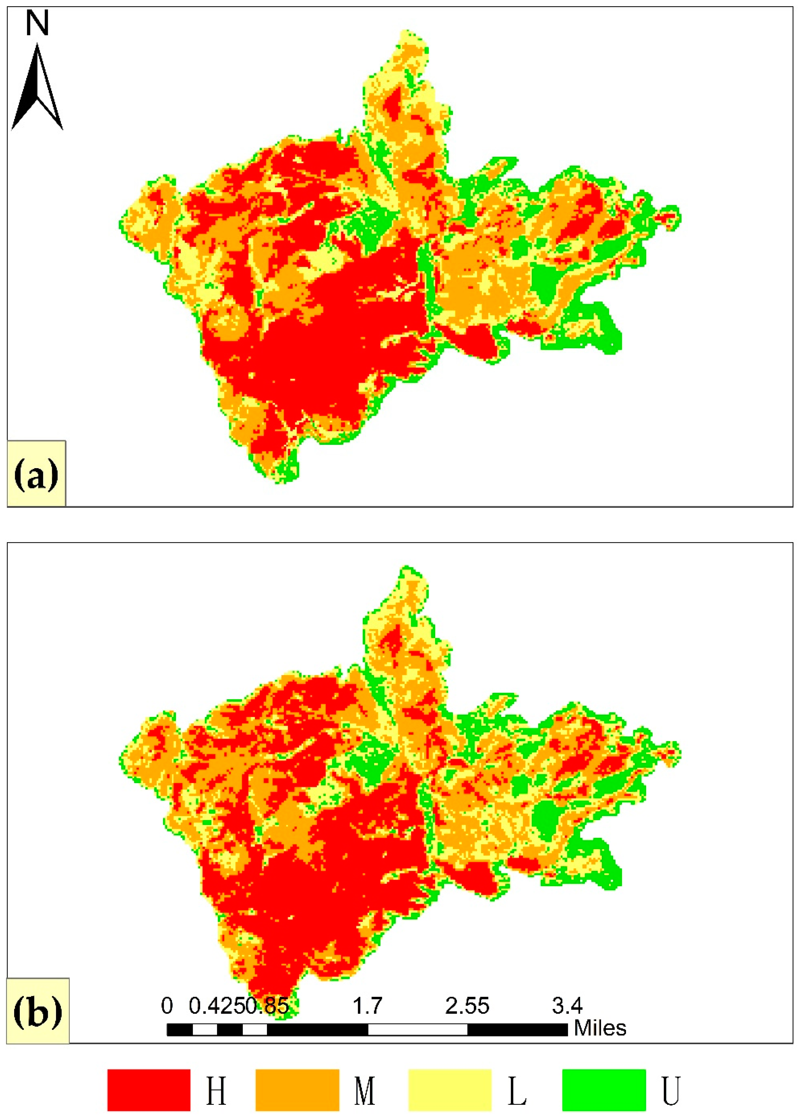
In this paper, the experiments were conducted separately according to the study area (European Mediterranean region; northwestern continental US). Data sources from different remote sensors were used in the two regions, which can further explore the applicability of the BAP method under different sensors in different regions. Each fire in the study area was classified separately for fire severity, without interfering with each other.
The training set and the test set required for classifying individual fires in the experiment were drawn randomly from the total dataset of corresponding fires. In this paper, according to the principle that the number of samples for each severity level is fixed, we drew the training set from the total dataset, with 300 samples for each level. Meanwhile, all the remaining data points in the total dataset were used as the validation set. The same sample size for each class in the training set avoids the imbalance between samples and conforms to the idea of collecting as many balanced samples as possible in practical work. We used the ERT classifier in our experiments to fit and classify the training and test sets.
For the classifier parameters mtry and ntree, after several tests, we found that the value of ntree did not improve the classification accuracy much after increasing up to 100, so the ntree parameter was fixed to 100. mtry is the quadratic root of the number of variables in the dataset. The above process of random sampling and classification was repeated 500 times.
The paper mainly uses Recall, Precision, F1-Score, OA (overall accuracy), and Kappa to evaluate the classification results of fire severity. Recall refers to, for all samples of a certain class, how many samples the classifier can find; Precision refers to, for a certain class of samples predicted by the classifier, how many samples belong to that class; F1-Score is a composite metric that reconciles Recall and Precision. OA and Kappa were used to evaluate the overall classification performance of fire severity. All indicators in the experiments were calculated based on the confusion matrix.
In this paper, we compared the BAP method with the conventional spectral indices-based method, which we refer to as the SI method. Firstly, in the SI method, different spectral indices are calculated using pre- or post-fire remote sensing images to form index images. Then, the direct superposition of all index images is involved in composing the fire severity feature images. Finally, the spectral index features are input into the ERT classifier to obtain classification and mapping results, similar to the process shown in Figure 6. A total of 10 spectral indices and their related variants (including the pre-fire, post-fire, and difference indices) were used in this paper, where the Burn Area Index (BAI) contains only the post-fire index. All used spectral indices are as follows: (1) The following indices use only the visible, near-infrared, or short-wave infrared bands: Normalized Burn Ratio (NBR) [16], Normalized Difference Vegetation Index (NDVI) [15], Normalized Difference Water Index (NDWI) [52], Visible Atmospherically Resistant Index (VARI) [53], Burn Area Index (BAI) [54]; (2) The following indices use red-edge bands: Chlorophyll Index red-edge (CIre) [55], Normalized Difference red-edge 1 (NDVIre1) [56], Normalized Difference red-edge 2 (NDVIre2) [57], Modified Simple Ratio red-edge (MSRre) [58], Modified Simple Ratio red-edge narrow (MSRren) [57].
The SI method for the Mediterranean region utilizing Sentinel-2 imagery uses 28 spectral index features (see Table 2). Whereas the Landsat-8 image used for the US region does not have a red-edge band, the SI method for this region uses only 13 spectral index features (See the first five lines of Table 2). The sample collection method, training and test set extraction method, and classifier parameter settings of the SI method were all consistent with those in the BAP method detailed in Section 3.2. It is worth noting that remote sensing data used in the SI method included both pre-fire and post-fire data (Table S3 in Supplementary Material for pre-fire image times).
We used the BAP and SI methods for fire severity mapping, and compared their processing results with real reference data to obtain visual differences. The feature extraction and classification processes were implemented using Python and MATLAB programming languages. ArcGIS was the cartographic tool used in this paper.

4. Results

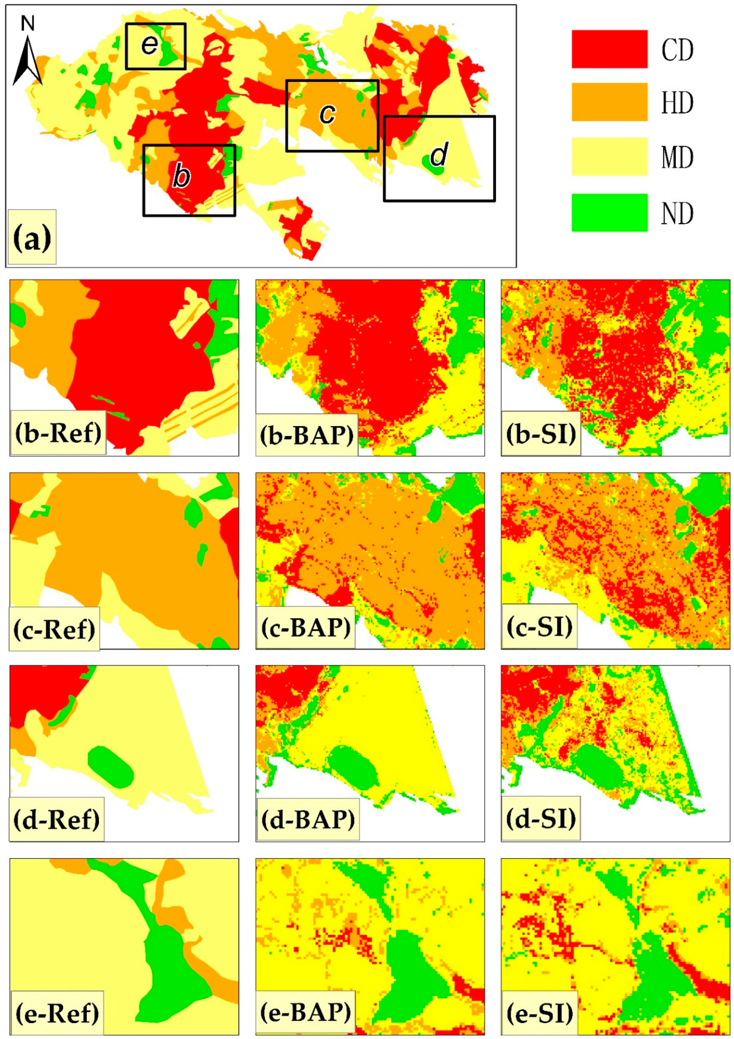
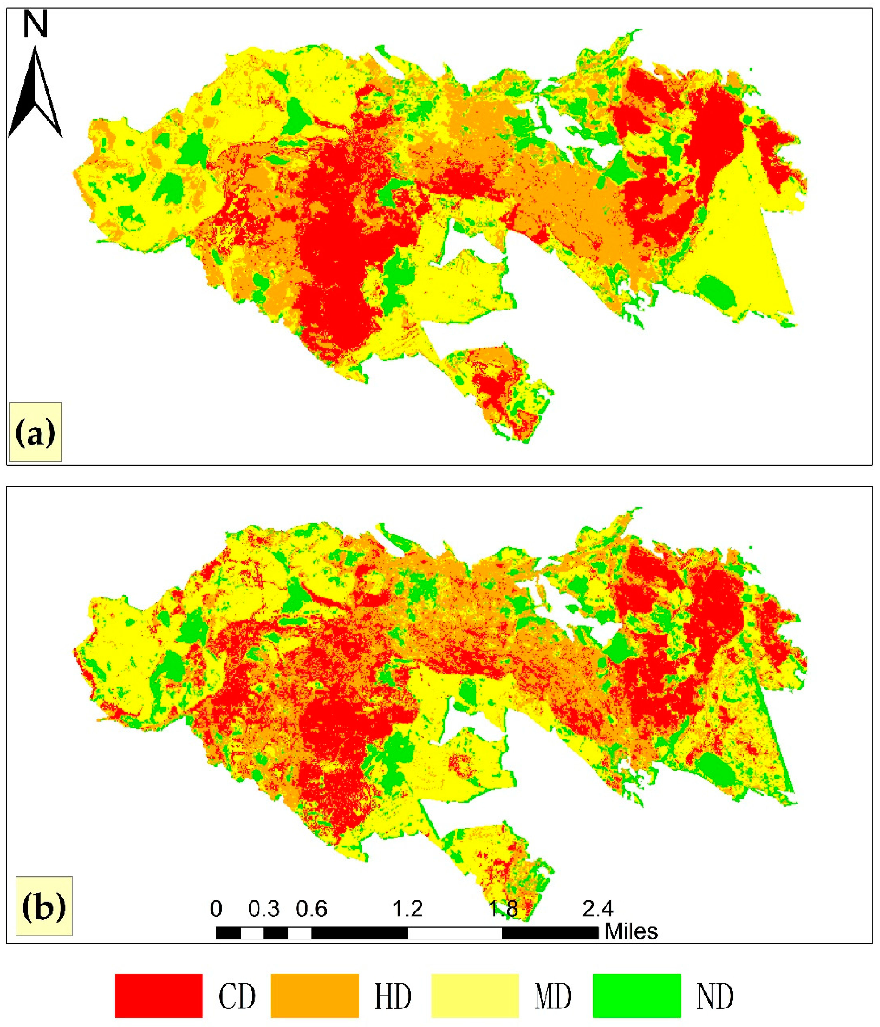
4.1. European Mediterranean Region

In this paper, the BAP and SI methods were used for feature extraction, and then the ERT classifier was used for classification, and the results are shown in Table 3. The values in Table 3 were the means of 500 randomized experiments (with 95% confidence intervals).
As can be seen from Table 3, for all fires in the Mediterranean region, the BAP method obtained better classifications than the SI method in terms of overall performance (OA improvement ranging from 0.2% to 14.3% (Difference Value) and Kappa improvement ranging from 0.3% to 19.5% (Difference Value)). It is worth noting that in these fires (e.g., EMSR213_A, EMSR213_S, EMSR216), there was a small improvement in the OA values of the BAP method compared to those of the SI method, while the OA values in the SI method were all very high.
For the Recall evaluation indicator, HD and MD were poorly classified among all fire severity levels, while CD and ND were the best. However, the HD and MD classes often greatly improve the comparisons of BAP vs. SI, and this should be related to these two classes’ relatively low Recall values. Still, it further illustrates that the BAP method can provide the classifier with more decision-making information about the classes where the SI method is relatively weak. However, on the other hand, the Recall values of HD and CD classes were high (0.894 to 0.999) in fires EMSR213_A, EMSR213_S, and EMSR216, and a negative boost in BAP was observed in these classes instead, which shows that the spectral information is more sensitive in these classes and the spectral information gives the classifier enough information for decision making.
For Precision, the most obvious difference from Recall is that the ND class performed the worst among multiple fires, which indicates that the classifier has a large misclassification error when classifying ND. HD and MD values were also low, and only the CD class had high precision values (0.808 to 0.996) in all fires. The F1 value per fire event was compared to that of Precision. It is worth noting that the fire EMSR213_P performs poorly in the ND, MD, and HD classes in all indicators, especially the Precision value for ND (0.182 for BAP and 0.140 for SI), but the BAP method shows better performance than the SI method in all fire events.
This paper produced the fire severity mapping results using Python and ArcGIS tools. The EMSR171 fire event result is described and illustrated in detail, as shown in Figure 7 and Figure 8. It can be seen that the BAP method can significantly improve the “salt-and-pepper” phenomenon seen in the traditional SI method, and the resulting severity level polygons were more regular and closer to the reference data (Figure 7b). In the mapping results of the SI method with many fragmented points, the CD class is mainly wrongly divided into CD and HD classes. In contrast, the BAP method labeled the entire region as a single CD class, close to the results on the reference map. The BAP method outperformed the SI method in the cases of other classes (Figure 7c–e).

4.2. Northwestern Continental United States Region

The BAP and SI methods were used for feature extraction, and then the ERT classifier was used for classification. The results are shown in Table 4, in which the values are the means of 500 randomized experiments (with 95% confidence intervals). As can be seen from Table 4, the BAP method was better than the SI method again (OA improvement ranged from 4.7% to 12.9% (Difference Value)). None of the OA values for the fire severity classification in the northwestern continental United States region are high (up to 0.793 for the region; up to 0.994 for the Mediterranean region), which should be related to reference data used in this study area. However, the Kappa values for all fires in the region were high (minimum value: 0.801 for the region; 0.419 for the Mediterranean region), and the variations were small.
According to the Recall classification evaluation indicator, U and H classes have the lowest values among all the fire severity levels. In contrast, the maximum value usually comes from the M class. The three BO, EL, and TW fires were consistent with those in the
Mediterranean region, and the BAP method showed the largest improvement over the SI method, which had smaller Recall values in U and H classes. In all severity levels of the three fires BA, HU, and WE, comparing the BAP method with the SI method, it was found that the Recall values were greatly improved. Only in the GR fire event was the Recall value decreased in the H class, while it was greatly improved in the M class.
Based on assessment via the Precision evaluation indicator, compared with the SI method, it can be seen that the BAP method had largely improved values in all fire severity levels in all fire events and only had smaller values in some M and H classes of several fire events (EL: M, GR: H, WE: H). At the same time, in the L class of fires BA and HU, BAP greatly improved compared to SI (BA: +0.171, HU: +0.224). It is worth noting that the Precision value of class L is the smallest among all fire severity levels of fires BA and HU. This further proves that the BAP method can provide more decision-making information for the classifier regarding fire severity levels than the SI method and, thus, produces better classification and mapping results.
In Figure 9 and Figure 10, taking the BO fire as an example, the results of fire severity mapping in the northwestern continental United States region are shown, including fire severity maps and detailed information for each severity level. Since there are some scattered points in the reference data itself, and the overall severity polygon is not very regular, the difference between the mapping results of the BAP and SI methods was not too large in terms of the overall visual effects. However, regarding all severity levels (Figure 9b–e), compared with the SI method, it can be found that the BAP method can obtain more regular severity regions with fewer internal fragmentation points.

5. Discussion

In this paper, we proposed a mathematical morphology-based spectral–spatial method named BAP. We selected 14 fires in two study areas, the Mediterranean region and the northwestern continental United States region, for fire severity mapping, in which Sentinel-2 and Landsat-8 satellite imagery data were used, respectively. There are obvious differences in these data in terms of spatial resolution, band spectral range, etc. The experimental results of the BAP method proposed in this paper and the traditional SI method show that spectral–spatial features can better describe the fire severity level than spectral index features. It is the first time that the spectral–spatial method has been used for fire severity mapping. The BAP method opens new paths in fire severity mapping and introduces a new application of spectral–spatial methods in fire severity classification mapping.

5.1. Performance of the BAP Method

In the two study areas of this paper, the BAP method has better classification results and can obtain better fire severity mapping results. Specifically, in the European Mediterranean region, the OA variation of the BAP spectral–spatial features combined with the ERT classifier ranges from 0.596 to 0.994, where only the EMSR213_P fire has a low OA value, and the OA of the other six fires is above 0.743. Meanwhile, OA values were lower in the continental US region, ranging from 0.595 to 0.793. However, OA values in the continental US region were relatively concentrated, and the OA values of half of the fires were above 0.749.
As for the individual classes, the classification systems of the two study areas are different, so they are discussed separately. According to the composite indicator F1, the CD class out of the four classes in the Mediterranean region performed best among all fires. This result is consistent with that of some previous studies showing higher average accuracy for extreme-intensity classes [25,59]. The F1 values of the other three classes were very low in some fires, especially the ND and MD classes. It is worth noting that the Precision values of the three classes were also very low, indicating that many data prediction results needed to be corrected in these fire classes. Several previous studies have mentioned the insufficient predictive performance of low- and medium-class severity [17,60,61]. It has been mentioned that higher misclassification rates usually occur in areas with dense canopy cover and rugged terrain [59]. This requires careful consideration of vegetation types and terrain factors, which must be further explored.
The severity classification system for the US region differs slightly from that of the European region in broad terms. It contains one class for the transition from unburned to low severity, and it does not have a separate class for completely destroyed severity. The F1 values of the low-severity L class for most fire events in the US region were the worst performing of all four classes, but these values were more stable and did not show minimal values. This result is also consistent with some previous studies [25,59]. The four classes of all seven fires in the US region, except the M class of the EL fire and the H class of the GR fire, had relatively high values in all three indicators (Recall, Precision, F1), and most of these values were above 0.749.
The BAP method introduces spatial–spectral features into fire severity classification. It achieves excellent classification results in different remote sensing images in different regions, which proves that the BAP method has good generalizability and can be applied to different data sources in different environments.

5.2. Comparison of BAP and SI Methods

The BAP method is the first to use spatial information for fire severity classification. To illustrate whether the inclusion of spatial information can help improve classification performance, we compared the BAP method with the SI method based on spectral features. In addition, the SI method is also the mainstream classification mapping method in the field of fire severity at present [22,62], and its comparison with BAP can also prove the advancement and superiority of the BAP method. Table 3 and Table 4 indicate that in all fire events, the BAP method is superior to the SI method in terms of classification’s overall accuracy, which has a high or low improvement. Moreover, evaluated from each class’s precision and recall values, the BAP method outperforms the SI method in most cases. In the Mediterranean study area, according to the Recall indicator, compared with the SI method, the BAP method’s boost was generally highest for MD and HD classes, which have relatively low values, while the ND and CD classes, which have relatively high values, showed smaller boosts or even negative boosts. For the seven fires in the US region, the degree of BAP’s boost over SI varies in each class. The class that has the greatest (or least) boost varies from fire event to fire event. It is worth noting that in a fire event, if the Recall value of a class increases the most, its Precision value will generally increase the most, and the same is true for the class with the smallest increase.
The above results are attributed to the fact that the BAP method considers the connectivity between image pixels and assigns the spatial features to the current pixel according to the morphological attribute similarity between the current pixel and its adjacent pixels in the neighborhood and further combines the spectral features to obtain the complete spectral–spatial features for the current pixel. In this way, the actual fire severity level of the pixel can be better described, and more accurate fire severity classification mapping results can be obtained. At the same time, it is also worth noting that due to the limited ability of morphological attributes and the complex spatial heterogeneity of fire severity, morphological attributes-based spectral–spatial features still need to be fully capable of describing fire severity levels, thus avoiding misclassification of fire severity.

5.3. Salt-and-Pepper Problem

We used the BAP and SI methods to map all 14 fires in two study areas separately. The mapping results show that the BAP method can effectively improve the salt-and-pepper problem in the homogeneous regions of fire severity maps. This is most evident in the EMSR171 fire (Figure 7 and Figure 8), especially in the regions labeled as CD or MD in the detailed diagram (Figure 7). It can be seen that the BAP method can merge the small fragmented and isolated regions into the surrounding large regions, making the regions more concentrated and complete in fire severity maps. On the one hand, this is due to the better classification accuracy of the BAP method compared to the SI method in the EMSR171 fire. On the other hand, it is also mainly due to the inclusion of spatial information in the BAP method, which makes homogeneous regions more aggregated through connected components. As shown in Figure 9 and Figure 10, the classification accuracy of BAP and SI in the BO fire is relatively close. However, the BAP method still greatly merges the small fragmented regions in SI into the larger surrounding homogeneous regions. The mapping results are more accurate and closer to the reference map.
The improvement effect of the BAP method by introducing the joint spatial–spectral information into fire severity mapping is significant. The “pretzel phenomenon” common in pixel-oriented mapping methods based on spectral features is effectively improved.

6. Conclusions

In this paper, a spectral–spatial method for fire severity classification, the Burn Attribute Profiles (BAP), is proposed to improve the accuracy of fire severity classification and mapping results. The spectral–spatial features of post-fire images are extracted using the BAP method, which automatically determines the threshold of the attributes and combines the spatial features with the spectral ones. Finally, an extremely randomized trees classifier is used to learn and predict fire severity maps. In our study, there were two study areas (the European Mediterranean region and the northwestern continental US region), each containing seven separate fires. Two types of different remote sensing data were used in the study areas (Mediterranean: Sentinel-2; US: Landsat-8) to evaluate the performance of the BAP method. According to the experimental results, BAP performed well in different data from different study areas and achieved high classification accuracy in most fires (10 out of 14 fires had OA greater than 70%). We then compared the BAP method with the mainstream SI method to assess whether including spatial information is beneficial for classifying fire severity. The results showed that the BAP method outperformed the SI method for all fires (OA improvement is 0.2–14.3% in the Mediterranean and 4.7–12.9% in the US). More results showed that the BAP method could improve the salt-and-pepper problem in SI mapping results.
However, the BAP method proposed in this paper still has much room for improvement. The attributes selected in this paper are frequently used in previous studies and performed well in our study for fire severity inversion. Therefore, exploring more attributes may lead to better classification results, reflecting the greater potential of the BAP method in fire severity classification. Furthermore, the attribute thresholds used in the paper are automatically determined. Thus, the number of coarsening and refining features is extremely large, among which there are bound to be many features that are not very useful for severity classification. In future work, the features obtained by BAP can be screened twice using genetic algorithms to reduce the number of features and computational effort.

Supplementary Materials

The following supporting information can be downloaded at: https://www.mdpi.com/article/10.3390/rs15030699/s1, Table S1: Classification performance testing of base image extraction methods for seven fires in the European Mediterranean region; Table S2: Classification performance tests for different grouping of attributes for seven fires in the European Mediterranean region; Table S3: Pre-fire remote sensing image times for each fire in the SI method.

Author Contributions

Conceptualization, X.R. and X.Y.; methodology, X.R. and X.Y.; visualization, X.R. and X.Y.; supervision, X.Y. and Y.W.; funding acquisition, X.Y. and Y.W.; writing—original draft preparation, X.R. and X.Y.; writing—review and editing, X.R., X.Y. and Y.W. All authors have read and agreed to the published version of the manuscript.

Funding

This research was funded by the National Natural Science Foundation of China, grant number 41101420 and 61271408.

Institutional Review Board Statement

Not applicable.

Informed Consent Statement

Not applicable.

Data Availability Statement

Publicly available datasets were analyzed in this study. These datasets can be found here: [https://code.earthengine.google.com/ (accessed on 25 June 2022)].

Acknowledgments

The authors would like to thank the European Space Agency (ESA) for providing the Sentinel-2 Level 1C products, the European Committee for providing the CEMS fire severity maps, the National Aeronautics and Space Administration (NASA) for providing the Landsat-8 products, and the USGS EROS Center and the USDA GTAC for jointly providing the MTBS fire severity maps. Furthermore, the authors would like to thank the handling editors and the anonymous reviewers for their valuable comments and suggestions, which significantly improved the quality of this paper.

Conflicts of Interest

The authors declare no conflict of interest.

References

  1. Seidl, R.; Schelhaas, M.-J.; Rammer, W.; Verkerk, P.J. Increasing forest disturbances in Europe and their impact on carbon storage. Nat. Clim. Chang. 2014, 4, 806–810. [Google Scholar] [CrossRef] [Green Version]
  2. Seidl, R.; Thom, D.; Kautz, M.; Martin-Benito, D.; Peltoniemi, M.; Vacchiano, G.; Wild, J.; Ascoli, D.; Petr, M.; Honkaniemi, J.; et al. Forest disturbances under climate change. Nat. Clim. Chang. 2017, 7, 395–402. [Google Scholar] [CrossRef] [Green Version]
  3. Barbosa, P.M.; Grégoire, J.-M.; Pereira, J.M.C. An algorithm for extracting burned areas from time series of AVHRR GAC data applied at a continental scale. Remote Sens. Environ. 1999, 69, 253–263. [Google Scholar] [CrossRef]
  4. van der Werf, G.R.; Randerson, J.T.; Giglio, L.; Collatz, G.J.; Kasibhatla, P.S.; Arellano, A.F., Jr. Interannual variability in global biomass burning emissions from 1997 to 2004. Atmos. Chem. Phys. 2006, 6, 3423–3441. [Google Scholar] [CrossRef] [Green Version]
  5. Burrows, N.D. Linking fire ecology and fire management in south-west Australian forest landscapes. For. Ecol. Manag. 2008, 255, 2394–2406. [Google Scholar] [CrossRef]
  6. Keeley, J.E. Fire intensity, fire severity and burn severity: A brief review and suggested usage. Int. J. Wildland Fire 2009, 18, 116–126. [Google Scholar] [CrossRef]
  7. Lentile, L.B.; Holden, Z.A.; Smith, A.M.S.; Falkowski, M.J.; Hudak, A.T.; Morgan, P.; Lewis, S.A.; Gessler, P.E.; Benson, N.C. Remote sensing techniques to assess active fire characteristics and post-fire effects. Int. J. Wildland Fire 2006, 15, 319–345. [Google Scholar] [CrossRef]
  8. Price, O.F.; Bradstock, R.A. The efficacy of fuel treatment in mitigating property loss during wildfires: Insights from analysis of the severity of the catastrophic fires in 2009 in victoria, Australia. J. Environ. Manag. 2012, 113, 146–157. [Google Scholar] [CrossRef]
  9. Bennett, L.T.; Bruce, M.J.; MacHunter, J.; Kohout, M.; Tanase, M.A.; Aponte, C. Mortality and recruitment of fire-tolerant eucalypts as influenced by wildfire severity and recent prescribed fire. For. Ecol. Manag. 2016, 380, 107–117. [Google Scholar] [CrossRef]
  10. White, J.D.; Ryan, K.C.; Key, C.C.; Running, S.W. Remote sensing of forest fire severity and vegetation recovery. Int. J. Wildland Fire 1996, 6, 125–136. [Google Scholar] [CrossRef] [Green Version]
  11. Epting, J.; Verbyla, D.; Sorbel, B. Evaluation of remotely sensed indices for assessing burn severity in interior Alaska using Landsat TM and etm+. Remote Sens. Environ. 2005, 96, 328–339. [Google Scholar] [CrossRef]
  12. Garcia-Llamas, P.; Suarez-Seoane, S.; Fernandez-Guisuraga, J.M.; Fernandez-Garcia, V.; Fernandez-Manso, A.; Quintano, C.; Taboada, A.; Marcos, E.; Calvo, L. Evaluation and comparison of Landsat 8, sentinel-2 and Deimos-1 remote sensing indices for assessing burn severity in Mediterranean fire-prone ecosystems. Int. J. Appl. Earth Obs. Geoinf. 2019, 80, 137–144. [Google Scholar] [CrossRef]
  13. Veraverbeke, S.; Hook, S.; Hulley, G. An alternative spectral index for rapid fire severity assessments. Remote Sens. Environ. 2012, 123, 72–80. [Google Scholar] [CrossRef]
  14. Saulino, L.; Rita, A.; Migliozzi, A.; Maffei, C.; Allevato, E.; Garonna, A.P.; Saracino, A. Detecting burn severity across Mediterranean forest types by coupling medium-spatial resolution satellite imagery and field data. Remote Sens. 2020, 12, 741. [Google Scholar] [CrossRef] [Green Version]
  15. Tucker, C.J. Red and photographic infrared linear combinations for monitoring vegetation. Remote Sens. Environ. 1979, 8, 127–150. [Google Scholar] [CrossRef] [Green Version]
  16. Lutes, D.C.; Keane, R.E.; Caratti, J.F.; Key, C.H.; Benson, N.C.; Sutherland, S.; Gangi, L.J. FIREMON: Fire effects monitoring and inventory system. In General Technical Report. RMRS-GTR-164-CD; Department of Agriculture, Forest Service, Rocky Mountain Research Station: Fort Collins, CO, USA, 2006; Volume 164, p. LA-1-55. [Google Scholar]
  17. Escuin, S.; Navarro, R.; Fernandez, P. Fire severity assessment by using NBR (normalized burn ratio) and NDVI (normalized difference vegetation index) derived from Landsat TM/ETM images. Int. J. Remote Sens. 2008, 29, 1053–1073. [Google Scholar] [CrossRef]
  18. Morgan, P.; Keane, R.E.; Dillon, G.K.; Jain, T.B.; Hudak, A.T.; Karau, E.C.; Sikkink, P.G.; Holden, Z.A.; Strand, E.K. Challenges of assessing fire and burn severity using field measures, remote sensing and modelling. Int. J. Wildland Fire 2014, 23, 1045. [Google Scholar] [CrossRef] [Green Version]
  19. Yin, C.M.; He, B.B.; Yebra, M.; Quan, X.W.; Edwards, A.C.; Liu, X.Z.; Liao, Z.M. Improving burn severity retrieval by integrating tree canopy cover into radiative transfer model simulation. Remote Sens. Environ. 2020, 236, 16. [Google Scholar] [CrossRef]
  20. Robichaud, P.R.; Lewis, S.A.; Laes, D.Y.M.; Hudak, A.T.; Kokaly, R.F.; Zamudio, J.A. Postfire soil burn severity mapping with hyperspectral image unmixing. Remote Sens. Environ. 2007, 108, 467–480. [Google Scholar] [CrossRef] [Green Version]
  21. Quintano, C.; Fernandez-Manso, A.; Roberts, D.A. Enhanced burn severity estimation using fine resolution ET and MESMA fraction images with machine learning algorithm. Remote Sens. Environ. 2020, 244, 16. [Google Scholar] [CrossRef]
  22. Dixon, D.J.; Callow, J.N.; Duncan, J.M.; Setterfield, S.A.; Pauli, N. Regional-scale fire severity mapping of eucalyptus forests with the Landsat archive. Remote Sens. Environ. 2022, 270, 112863. [Google Scholar] [CrossRef]
  23. Collins, L.; Mc Carthy, G.; Mellor, A.; Newell, G.; Smith, L. Training data requirements for fire severity mapping using Landsat imagery and random forest. Remote Sens. Environ. 2020, 245, 14. [Google Scholar] [CrossRef]
  24. Belgiu, M.; Dragut, L. Random forest in remote sensing: A review of applications and future directions. ISPRS J. Photogramm. Remote Sens. 2016, 114, 24–31. [Google Scholar] [CrossRef]
  25. Collins, L.; Griffioen, P.; Newell, G.; Mellor, A. The utility of random forests for wildfire severity mapping. Remote Sens. Environ. 2018, 216, 374–384. [Google Scholar] [CrossRef]
  26. Tran, N.B.; Tanase, M.A.; Bennett, L.T.; Aponte, C. Fire-severity classification across temperate Australian forests: Random forests versus spectral index thresholding. In Proceedings of the Conference on Remote Sensing for Agriculture, Ecosystems, and Hydrology XXI held at SPIE Remote Sensing, Strasbourg, France, 9–11 September 2019. [Google Scholar]
  27. Cutler, D.R.; Edwards Jr, T.C.; Beard, K.H.; Cutler, A.; Hess, K.T.; Gibson, J.; Lawler, J.J. Random forests for classification in ecology. Ecology 2007, 88, 2783–2792. [Google Scholar] [CrossRef] [PubMed]
  28. Syifa, M.; Panahi, M.; Lee, C.W. Mapping of post-wildfire burned area using a hybrid algorithm and satellite data: The case of the camp fire wildfire in California, USA. Remote Sens. 2020, 12, 623. [Google Scholar] [CrossRef] [Green Version]
  29. Yu, Q.; Gong, P.; Clinton, N.; Biging, G.; Kelly, M.; Schirokauer, D. Object-based detailed vegetation classification. With airborne high spatial resolution remote sensing imagery. Photogramm. Eng. Remote Sens. 2006, 72, 799–811. [Google Scholar] [CrossRef] [Green Version]
  30. Amos, C.; Petropoulos, G.P.; Ferentinos, K.P. Determining the use of Sentinel-2a MSI for wildfire burning & severity detection. Int. J. Remote Sens. 2019, 40, 905–930. [Google Scholar] [CrossRef]
  31. Wu, J. Effects of changing scale on landscape pattern analysis: Scaling relations. Landsc. Ecol. 2004, 19, 125–138. [Google Scholar] [CrossRef]
  32. Hu, X.; Xu, H. A new remote sensing index for assessing the spatial heterogeneity in urban ecological quality: A case from Fuzhou city, china. Ecol. Indic. 2018, 89, 11–21. [Google Scholar] [CrossRef]
  33. Fauvel, M.; Benediktsson, J.A.; Chanussot, J.; Sveinsson, J.R. Spectral and spatial classification of hyperspectral data using SVMs and morphological profiles. IEEE Trans. Geosci. Remote Sens. 2008, 46, 3804–3814. [Google Scholar] [CrossRef] [Green Version]
  34. Li, J.; Bioucas-Dias, J.M.; Plaza, A. Spectral-spatial hyperspectral image segmentation using subspace multinomial logistic regression and Markov random fields. IEEE Trans. Geosci. Remote Sens. 2012, 50, 809–823. [Google Scholar] [CrossRef]
  35. Wang, P.; Wang, L.G.; Leung, H.; Zhang, G. Super-resolution mapping based on spatial-spectral correlation for spectral imagery. IEEE Trans. Geosci. Remote Sens. 2021, 59, 2256–2268. [Google Scholar] [CrossRef]
  36. Ghamisi, P.; Dalla Mura, M.; Benediktsson, J.A. A survey on spectral-spatial classification techniques based on attribute profiles. IEEE Trans. Geosci. Remote Sens. 2015, 53, 2335–2353. [Google Scholar] [CrossRef]
  37. Dalla Mura, M.; Benediktsson, J.A.; Waske, B.; Bruzzone, L. Morphological attribute profiles for the analysis of very high resolution images. IEEE Trans. Geosci. Remote Sens. 2010, 48, 3747–3762. [Google Scholar] [CrossRef]
  38. Pedergnana, M.; Marpu, P.R.; Mura, M.D.; Benediktsson, J.A.; Bruzzone, L. Classification of remote sensing optical and LiDAR data using extended attribute profiles. IEEE J. Sel. Top. Signal Process. 2012, 6, 856–865. [Google Scholar] [CrossRef]
  39. Shang, X.D.; Song, M.P.; Wang, Y.L.; Yu, C.Y.; Yu, H.Y.; Li, F.; Chang, C.I. Target-constrained interference-minimized band selection for hyperspectral target detection. IEEE Trans. Geosci. Remote Sens. 2021, 59, 6044–6064. [Google Scholar] [CrossRef]
  40. Dalla Mura, M.; Benediktsson, J.A.; Waske, B.; Bruzzone, L. Extended profiles with morphological attribute filters for the analysis of hyperspectral data. Int. J. Remote Sens. 2010, 31, 5975–5991. [Google Scholar] [CrossRef]
  41. Licciardi, G.A.; Villa, A.; Dalla Mura, M.; Bruzzone, L.; Chanussot, J.; Benediktsson, J.A. Retrieval of the height of buildings from Worldview-2 multi-angular imagery using attribute filters and geometric invariant moments. IEEE J. Sel. Top. Appl. Earth Obs. Remote Sens. 2012, 5, 71–79. [Google Scholar] [CrossRef] [Green Version]
  42. Falco, N.; Dalla Mura, M.; Bovolo, F.; Benediktsson, J.A.; Bruzzone, L. Change detection in VHR images based on morphological attribute profiles. IEEE Geosci. Remote Sens. Lett. 2013, 10, 636–640. [Google Scholar] [CrossRef]
  43. Ghamisi, P.; Maggiori, E.; Li, S.T.; Souza, R.; Tarabalka, Y.; Moser, G.; De Giorgi, A.; Fang, L.Y.; Chen, Y.S.; Chi, M.M.; et al. New frontiers in spectral-spatial hyperspectral image classification: The latest advances based on mathematical morphology, Markov random fields, segmentation, sparse representation, and deep learning. IEEE Geosci. Remote Sens. Mag. 2018, 6, 10–43. [Google Scholar] [CrossRef]
  44. Marpu, P.R.; Pedergnana, M.; Dalla Mura, M.; Benediktsson, J.A.; Bruzzone, L. Automatic generation of standard deviation attribute profiles for spectral-spatial classification of remote sensing data. IEEE Geosci. Remote Sens. Lett. 2013, 10, 293–297. [Google Scholar] [CrossRef]
  45. Ghamisi, P.; Benediktsson, J.A.; Cavallaro, G.; Plaza, A. Automatic framework for spectral-spatial classification based on supervised feature extraction and morphological attribute profiles. IEEE J. Sel. Top. Appl. Earth Obs. Remote Sens. 2014, 7, 2147–2160. [Google Scholar] [CrossRef]
  46. Kolden, C.A.; Smith, A.M.S.; Abatzoglou, J.T. Limitations and utilisation of monitoring trends in burn severity products for assessing wildfire severity in the USA. Int. J. Wildland Fire 2015, 24, 1023–1028. [Google Scholar] [CrossRef]
  47. Dalla Mura, M.; Villa, A.; Benediktsson, J.A.; Chanussot, J.; Bruzzone, L. Classification of hyperspectral images by using extended morphological attribute profiles and independent component analysis. IEEE Geosci. Remote Sens. Lett. 2011, 8, 542–546. [Google Scholar] [CrossRef] [Green Version]
  48. Huang, X.; Guan, X.H.; Benediktsson, J.A.; Zhang, L.P.; Li, J.; Plaza, A.; Dalla Mura, M. Multiple morphological profiles from multicomponent-base images for hyperspectral image classification. IEEE J. Sel. Top. Appl. Earth Obs. Remote Sens. 2014, 7, 4653–4669. [Google Scholar] [CrossRef]
  49. Geurts, P.; Ernst, D.; Wehenkel, L. Extremely randomized trees. Mach. Learn. 2006, 63, 3–42. [Google Scholar] [CrossRef] [Green Version]
  50. Bunting, P.; Rosenqvist, A.; Lucas, R.M.; Rebelo, L.M.; Hilarides, L.; Thomas, N.; Hardy, A.; Itoh, T.; Shimada, M.; Finlayson, C.M. The global mangrove watch: A new 2010 global baseline of mangrove extent. Remote Sens. 2018, 10, 1669. [Google Scholar] [CrossRef] [Green Version]
  51. Soltaninejad, M.; Yang, G.; Lambrou, T.; Allinson, N.; Jones, T.L.; Barrick, T.R.; Howe, F.A.; Ye, X.J. Automated brain tumour detection and segmentation using superpixel-based extremely randomized trees in FLAIR MRI. Int. J. Comput. Assist. Radiol. Surg. 2017, 12, 183–203. [Google Scholar] [CrossRef] [Green Version]
  52. Gao, B.C. NDWI—A normalized difference water index for remote sensing of vegetation liquid water from space. Remote Sens. Environ. 1996, 58, 257–266. [Google Scholar] [CrossRef]
  53. Gitelson, A.A.; Kaufman, Y.J.; Stark, R.; Rundquist, D. Novel algorithms for remote estimation of vegetation fraction. Remote Sens. Environ. 2002, 80, 76–87. [Google Scholar] [CrossRef] [Green Version]
  54. Chuvieco, E.; Martin, M.P.; Palacios, A. Assessment of different spectral indices in the red-near-infrared spectral domain for burned land discrimination. Int. J. Remote Sens. 2002, 23, 5103–5110. [Google Scholar] [CrossRef]
  55. Gitelson, A.A.; Gritz, Y.; Merzlyak, M.N. Relationships between leaf chlorophyll content and spectral reflectance and algorithms for non-destructive chlorophyll assessment in higher plant leaves. J. Plant Physiol. 2003, 160, 271–282. [Google Scholar] [CrossRef] [PubMed]
  56. Gitelson, A.; Merzlyak, M.N. Spectral reflectance changes associated with autumn senescence of Aesculus-hippocastanum L. and Acer-platanoides L. leaves-spectral features and relation to chlorophyll estimation. J. Plant Physiol. 1994, 143, 286–292. [Google Scholar] [CrossRef]
  57. Fernández-Manso, A.; Fernández-Manso, O.; Quintano, C. Sentinel-2a red-edge spectral indices suitability for discriminating burn severity. Int. J. Appl. Earth Obs. Geoinf. 2016, 50, 170–175. [Google Scholar] [CrossRef]
  58. Chen, J.M. Evaluation of vegetation indices and a modified simple ratio for boreal applications. Can. J. Remote Sens. 1996, 22, 229–242. [Google Scholar] [CrossRef]
  59. Gibson, R.; Danaher, T.; Hehir, W.; Collins, L. A remote sensing approach to mapping fire severity in south-eastern Australia using Sentinel 2 and random forest. Remote Sens. Environ. 2020, 240, 13. [Google Scholar] [CrossRef]
  60. Franco, M.G.; Mundo, I.A.; Veblen, T.T. Field-validated burn-severity mapping in north Patagonian forests. Remote Sens. 2020, 12, 214. [Google Scholar] [CrossRef] [Green Version]
  61. Quintano, C.; Fernández-Manso, A.; Fernández-Manso, O. Combination of Landsat and Sentinel-2 MSI data for initial assessing of burn severity. Int. J. Appl. Earth Obs. Geoinf. 2018, 64, 221–225. [Google Scholar] [CrossRef]
  62. Van Gerrevink, M.J.; Veraverbeke, S. Evaluating the hyperspectral sensitivity of the differenced normalized burn ratio for assessing fire severity. Remote Sens. 2021, 13, 4611. [Google Scholar] [CrossRef]
Figure 1. Study area and the location of the fires in (a) the European Mediterranean region; (b) the northwestern continental United States region.
Remotesensing 15 00699 g001
Figure 2. Fire severity reference maps of (a) the EMSR171 fire (located in the European Mediterranean region. CD: Completely Destroyed; HD: Highly Damaged; MD: Moderately Damaged; ND: Negligible to Slight Damage); (b) the BO fire (located in the northwestern continental United States. U: Unburned to Low; L: Low; M: Moderate; H: High).
Remotesensing 15 00699 g002
Figure 3. Proposed fire severity mapping scheme.
Remotesensing 15 00699 g003
Figure 4. Morphological Attribute Profiles (APs) and Extended APs (EAPs) for base image X .
Remotesensing 15 00699 g004
Figure 5. Burn Attribute Profiles (BAP) feature curves for the four classes in the EMSR171 fire: (a) CD: Completely Destroyed; (b) HD: Highly Damaged; (c) MD: Moderately Damaged; (d) ND: Negligible to Slight Damage. Shown for each class with one sample point taken randomly, and each band corresponds to a value within 0~255.
Remotesensing 15 00699 g005
Figure 6. The sample collection process for the EMSR171 fire.
Remotesensing 15 00699 g006
Figure 7. Detailed display of EMSR171 fire mapping results: (a) fire severity reference map; (b) Detailed display of CD class; (c) HD class; (d) MD class; (e) ND class. Ref: reference map; BAP: Fire severity mapping generated by BAP method; SI: Fire severity mapping generated by SI method.
Remotesensing 15 00699 g007
Figure 8. Comparison of EMSR171 fire severity mapping results of (a) BAP method; (b) SI method.
Remotesensing 15 00699 g008
Figure 9. Detailed display of BO fire mapping results: (a) fire severity reference map; (b) Detailed display of H class; (c) M class; (d) L class; (e) U class. Ref: reference map; BAP: Fire severity mapping generated by BAP method; SI: Fire severity mapping generated by SI method.
Remotesensing 15 00699 g009
Figure 10. Comparison of BO fire severity mapping results of (a) BAP method; (b) SI method.
Remotesensing 15 00699 g010
Table 1. The occurrence times of all 14 fires, the acquisition times of the corresponding remote sensing images, and the number of sample points for fire severity classes.
FireStart TimePost-Fire
Image Time
Sample Points for Fire Severity Classes
NDMDHDCDTotal
European Mediterranean
EMSR1326 August 2015
–11 August 2015
11 August 201520,70740,918141,066506,953709,644
EMSR16916 June 2016
–2 July 2016
12 July 201659,80665,92170,536147,988344,251
EMSR1714 July 2016
–26 July 2016
28 July 2016458563,83427,69731,999128,115
EMSR213_A11 July 2017
–29 August 2017
13 September 201768039602654844915,743
EMSR213_P11 July 2017
–9 August 2017
11 August 2017652523,64547,14159,481136,792
EMSR213_S11 July 2017
–31 August 2017
2 September 201782117701041818211,814
EMSR21627 July 2017
–4 August 2017
7 August 20171957309115817677396
Northwestern Continental United States
ULMHTotal
BA2 August 201420 July 201525613717113711528567
BO11 August 201524 July 2016130913223724742813,783
EL14 August 201521 August 2015427554,9717074136167,681
GR14 August 201527 June 2016381413,8023952158523,153
HU10 August 201622 July 20172745170489627398084
TW19 August 20154 September 2015242124,4126332137034,535
WE14 August 201524 July 201642537727581722,72140,518
Table 2. The spectral indices used for SI Method in this study. The indices considered for the classification include the pre- and post-fire difference indices (denoted by Δ) and the pre- and post-fire indices (denoted by “pre” or “post”).
IndexEquationReferenceIndices Considered
NBR N I R S W I R 2 N I R + S W I R 2 [16] NBR p r e ,   NBR p o s t ,   Δ NBR
NDVI N I R R N I R + R [15] NDVI p r e ,   NDVI p o s t ,   Δ NDVI
NDWI N I R S W I R 1 N I R + S W I R 1 [52] NDWI p r e ,   NDWI p o s t ,   Δ NDWI
VARI G R G + R B [53] VARI p r e ,   VARI p o s t ,   Δ VARI
BAI 1 ( 0.1 R ) 2 + ( 0.06 N I R ) 2 [54] Δ BAI
CIre Red   Edge   3 Red   Edge   1 1 [55] CIre p r e ,   CIre p o s t ,   Δ CIre
NDVIre1 N I R Red   Edge   1 N I R + Red   Edge   1 [56] NDVIre 1 p r e ,   NDVIre 1 p o s t ,   Δ NDVIre 1
NDVIre2 N I R Red   Edge   2 N I R + Red   Edge   2 [57] NDVIre 2 p r e ,   NDVIre 2 p o s t ,   Δ NDVIre 2
MSRre ( N I R / Red   Edge   1 ) 1 ( N I R / Red   Edge   1 ) + 1 [58] MSRre p r e ,   MSRre p o s t ,   Δ MSRre
MSRren ( Red   Edge   4 / Red   Edge   1 ) 1 ( Red   Edge   4 / Red   Edge   1 ) + 1 [57] MSRren p r e ,   MSRren p o s t ,   Δ MSRren
Table 3. Performance comparison of fire severity classifications using BAP and Spectral Indices (SI) methods for each fire in the European Mediterranean region. ND: Negligible to Slight Damage; MD: Moderately Damaged; HD: Highly Damaged; CD: Completely Destroyed.
IndicatorsClassEMSR132EMSR171EMSR169EMSR213_AEMSR213_PEMSR213_SEMSR216
BAPSIBAPSIBAPSIBAPSIBAPSIBAPSIBAPSI
RecallND0.8850.8300.8970.8130.8020.6830.9290.9110.5800.5060.9630.9190.9940.996
MD0.7320.5880.7180.6210.6810.5280.9470.9200.4970.4660.9150.9080.9930.987
HD0.6660.5540.7090.5840.6520.4480.9250.8920.4700.3840.8940.8960.9960.990
CD0.8540.8340.8000.6900.8370.7160.9680.9690.7370.7040.9440.9470.9990.995
PrecisionND0.5650.3950.3330.2310.6660.5530.5930.5840.1820.1400.8810.8430.9930.992
MD0.3960.3120.8850.8490.6490.5060.9720.9540.4550.3950.9620.9610.9950.996
HD0.5920.5230.6020.5050.6550.4030.8860.8400.5960.5470.5660.5690.9950.980
CD0.9780.9620.8080.6520.9330.8620.9960.9960.8200.7910.9960.9960.9950.983
F1ND0.6890.5350.4850.3600.7270.6110.7230.7110.2770.2200.9200.8790.9930.994
MD0.5140.4080.7930.7170.6640.5160.9590.9360.4750.4270.9380.9340.9940.991
HD0.6260.5370.6510.5410.6530.4240.9050.8650.5250.4510.6930.6960.9950.985
CD0.9110.8930.8040.6700.8820.7820.9820.9820.7760.7450.9690.9710.9970.989
Kappa0.6220.5350.6200.4750.6700.4750.9260.9050.4190.3520.8610.8580.9920.986
OA0.8100.7640.7430.6370.7630.6200.9550.9430.5960.5440.9380.9360.9940.991
Table 4. Performance comparison of fire severity classification using BAP and SI methods for each fire within the northwestern continental US region. U: Unburned to Low; L: Low; M: Moderate; H: High.
IndicatorsClassBABOELGRHUTWWE
BAPSIBAPSIBAPSIBAPSIBAPSIBAPSIBAPSI
RecallU0.7780.6860.7480.6390.8190.7790.7610.7450.7330.6240.8140.7620.7240.675
L0.8550.7030.8330.7380.8440.8420.8410.7450.8460.7040.7480.7500.8350.751
M0.9400.8380.9060.8760.9350.9330.9450.8440.9280.8060.9200.9020.9090.879
H0.8040.7390.8260.8010.5510.4430.5850.6180.8990.8600.6070.4530.7320.727
PrecisionU0.8750.8090.5770.4470.9850.9790.9310.9120.7140.6060.9500.9480.8270.769
L0.6690.4980.8000.7200.5300.4740.7050.6090.6020.3780.5880.5710.6080.523
M0.9440.8730.9760.9550.3160.3920.8460.7250.9860.9600.6060.5660.9820.976
H0.8300.7710.8500.8260.7020.6000.6930.7230.8740.8290.7410.6060.7780.786
F1U0.8240.7420.6510.5260.8940.8680.8370.8200.7230.6140.8760.8450.7720.719
L0.7500.5830.8160.7290.6510.6060.7670.6700.7030.4920.6580.6480.7030.616
M0.9420.8550.9400.9140.4720.5510.8930.7790.9560.8760.7300.6950.9440.925
H0.8300.7430.8710.8170.8320.7970.7990.7710.8530.7580.8140.7740.8550.820
Kappa0.8570.8070.8770.8530.9710.9330.8510.8710.8500.8010.9550.9180.8300.857
OA0.7490.6230.7890.7020.5950.5340.6750.6280.7930.6640.6300.5720.7700.717
Disclaimer/Publisher’s Note: The statements, opinions and data contained in all publications are solely those of the individual author(s) and contributor(s) and not of MDPI and/or the editor(s). MDPI and/or the editor(s) disclaim responsibility for any injury to people or property resulting from any ideas, methods, instructions or products referred to in the content.

