
Comparison of Three Methods for Distinguishing Glacier Zones Using Satellite SAR Data
 , , , , , and
Abstract
:1. Introduction
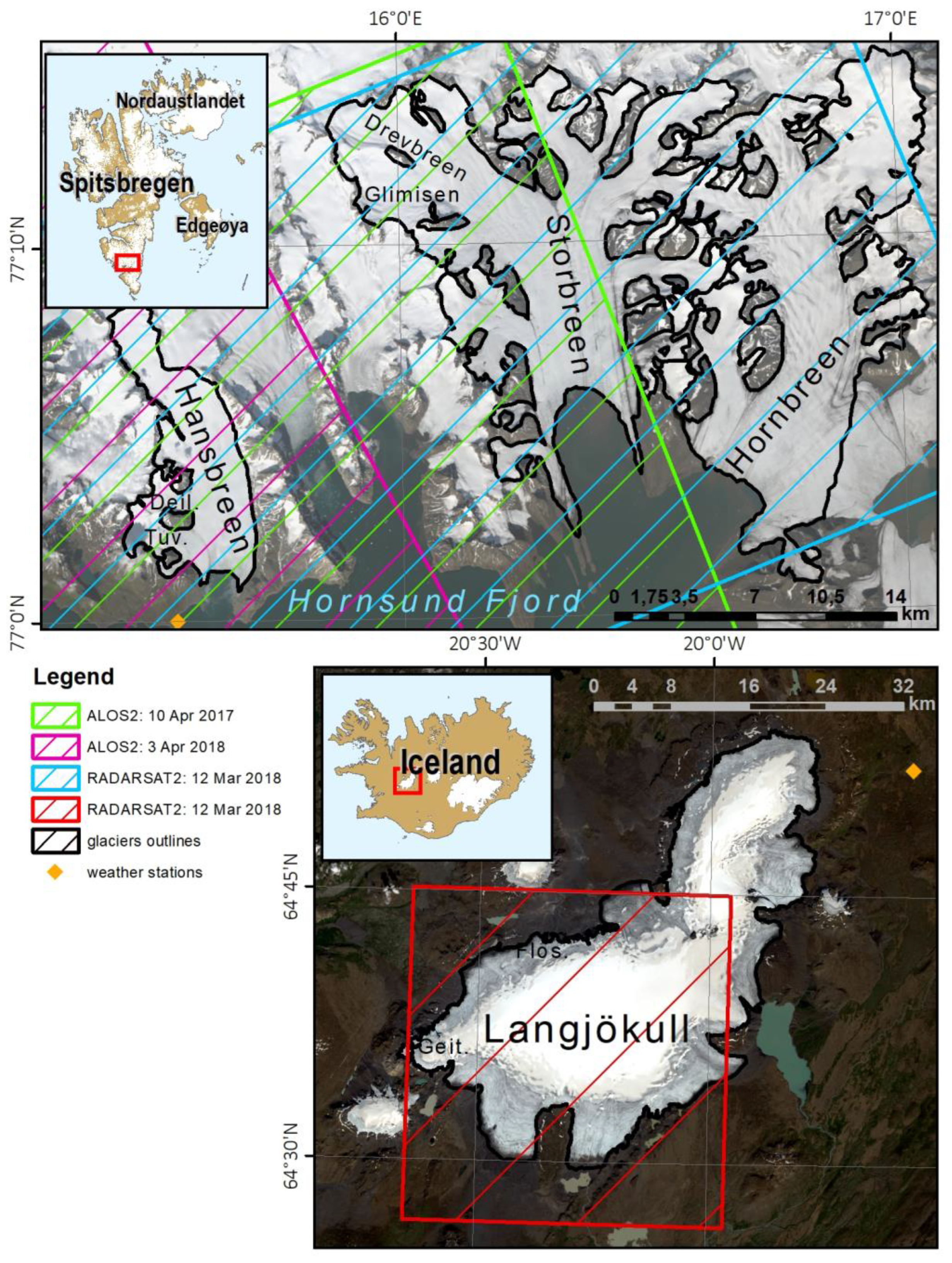
2. Study Sites
3. Materials and Methods
3.1. Materials
3.1.1. SAR Data
3.1.2. GPR Data
3.1.3. Shallow Glacier Cores
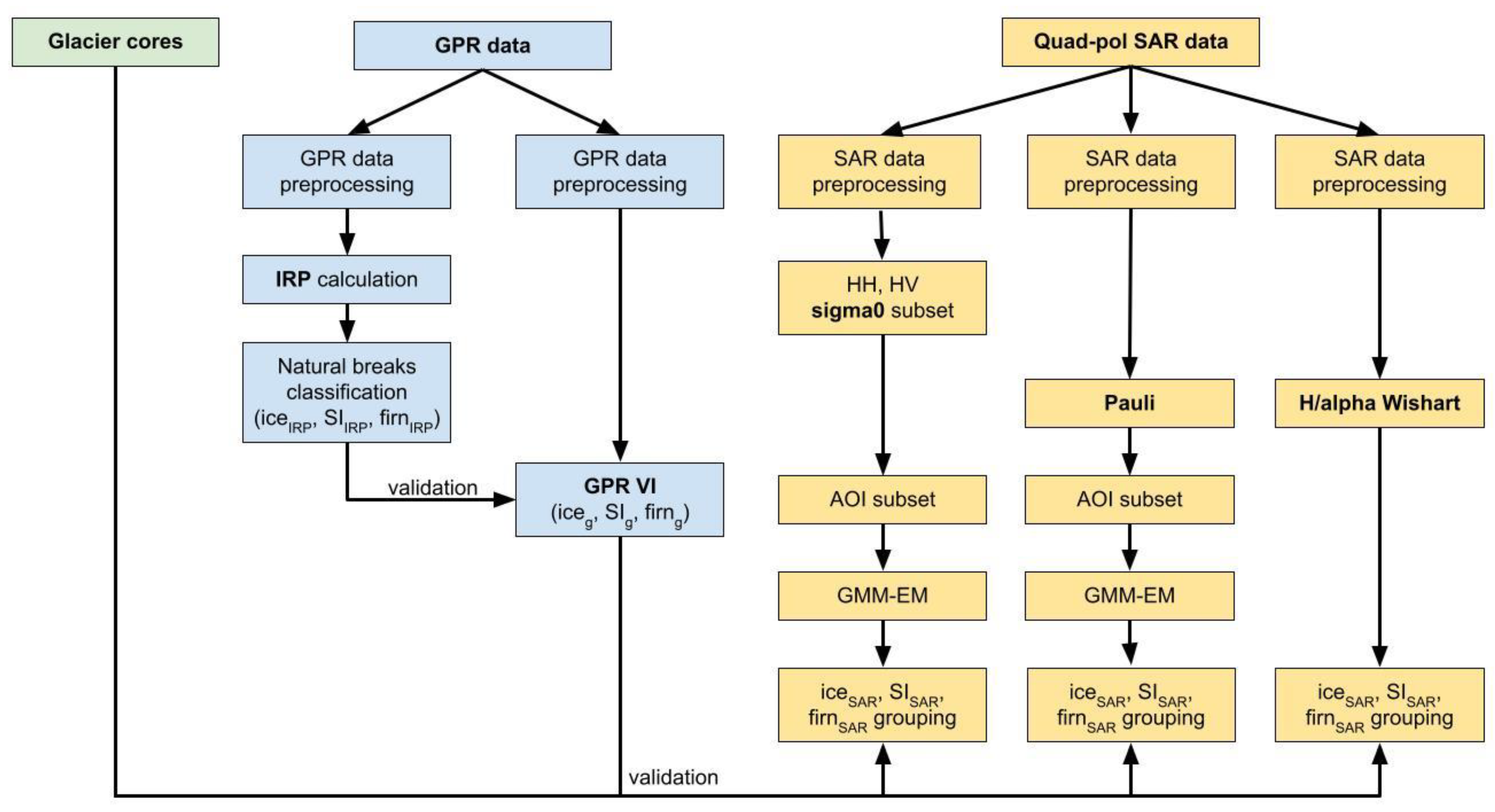
3.2. Methods
3.2.1. GPR VI and IRP Natural Breaks Classification
3.2.2. GMM-EM Classification of Dual-Pol SAR Sigma0
3.2.3. GMM-EM Classification of Quad-Pol SAR Pauli Decomposition
3.2.4. H/α Wishart Segmentation of Quad-Pol SAR Data
4. Results
4.1. Analysis of Terrestrial Data
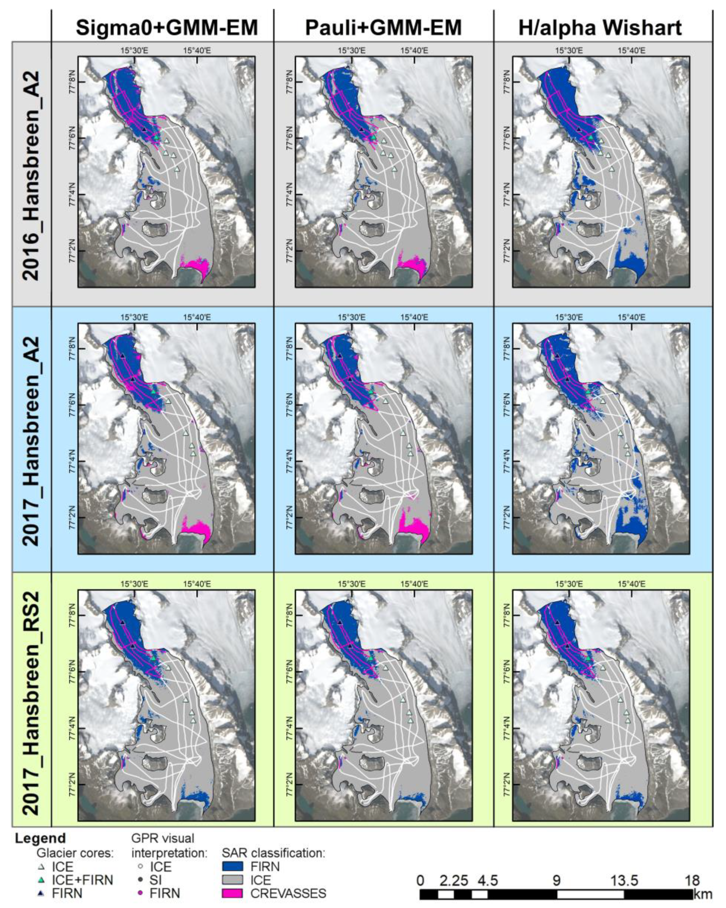
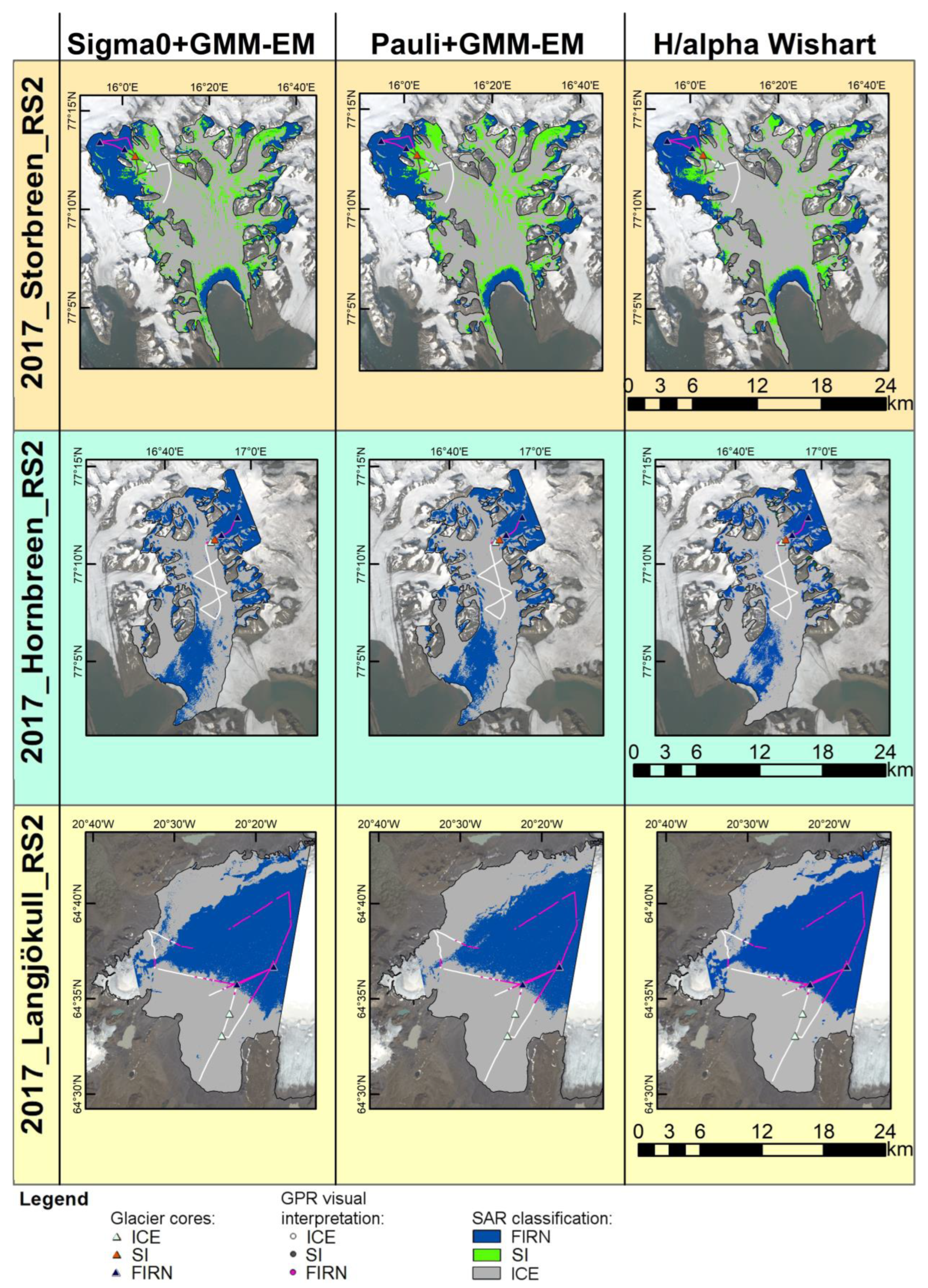
4.2. Distinguishing Glacier Zones Based on SAR Data
4.2.1. GMM-EM Classification of Dual-Pol SAR Sigma0
4.2.2. GMM-EM Classification of Quad-Pol SAR Pauli Decomposition
4.2.3. H/α Wishart Segmentation of Quad-Pol SAR Data
5. Discussion
6. Conclusions
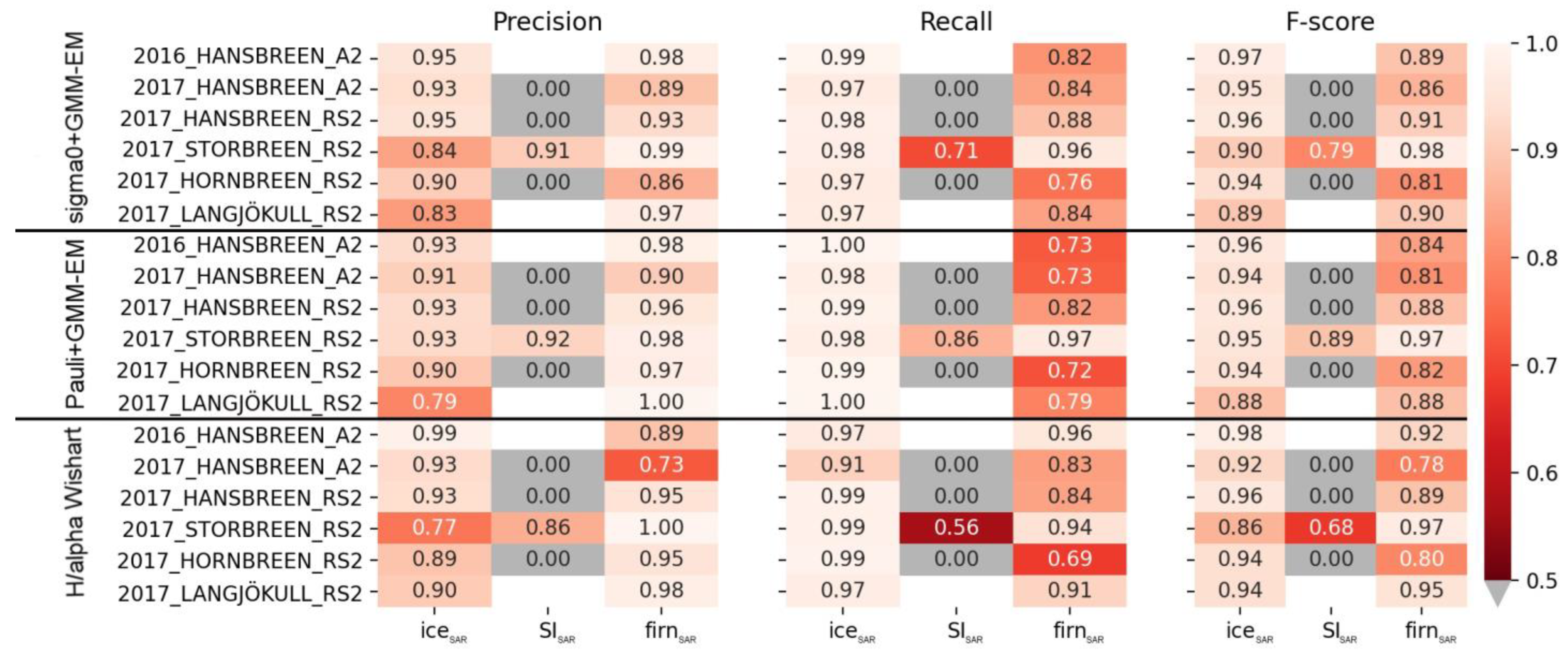
- The results of the unsupervised classification (Gaussian Mixture Model–Expectation Maximization algorithm) of both HH/HV sigma0 and Pauli decomposition are the most promising for distinguishing glacier zones.
- Firn on analyzed SAR images is better represented by the classification results of dual-pol sigma0 than by quad-pol Pauli decomposition and classification.
- Better results for the detection of the SI of Storbreen were obtained by the unsupervised classification of quad-pol Pauli decomposition than of dual-pol sigma0. However, to confirm that the unsupervised classification of Pauli decomposition performs better than other methods in distinguishing SI, more tests on different glaciers are needed.
- The H/α Wishart method gave less satisfactory results than the unsupervised classification of either sigma0 or Pauli decomposition. This is due to inconsistent results with regard to distinguishing glacier zones on Hansbreen, which were assessed based on terrestrial data and accuracy metrics. The inconsistency in the H/α Wishart results is probably determined by either the fixed boundaries of the H–α plane where the cluster centers are located or by differences in the processing workflow in comparison to the unsupervised classification of sigma0 or Pauli.
- To detect a firn zone on SAR images, shallower-penetrating C-band RADARSAT-2 data give better results than L-band ALOS-2 PALSAR-2 when the unsupervised classification of either sigma0 or Pauli decomposition is used.
- The unsupervised classification of dual-pol sigma0 is not outperformed by the results of the classification of quad-pol SAR data and polarimetric methods. This is especially promising in terms of the better availability of dual-pol than quad-pol SAR data.
- The heterogeneity of the glacier ice body could potentially be distinguished by L-band SAR data and the application of the unsupervised classification of either sigma0 or Pauli decomposition. To support this, more tests are needed, especially for glaciers with highly crevassed areas.
- Despite the differences in morphology or climate conditions of the land ice masses of Svalbard and Iceland, the assessed quality of the results of the tested methods are comparable.
Author Contributions
Funding
Institutional Review Board Statement
Informed Consent Statement
Data Availability Statement
Acknowledgments
Conflicts of Interest
References
- The European Space Agency. CEOS. Committee on Earth Observation Satellites Database. Available online: http://database.eohandbook.com/ (accessed on 10 July 2021).
- Lewis, A.; Lymburner, L.; Purss, M.B.J.; Brooke, B.; Evans, B.; Ip, A.; Dekker, A.G.; Irons, J.R.; Minchin, S.; Mueller, N.; et al. Rapid, high-resolution detection of environmental change over continental scales from satellite data—The Earth Observation Data Cube. Int. J. Digit. Earth 2016, 9, 106–111. [Google Scholar] [CrossRef]
- Amani, M.; Ghorbanian, A.; Ahmadi, S.A.; Kakooei, M.; Moghimi, A.; Mirmazloumi, S.M.; Moghaddam, S.H.A.; Mahdavi, S.; Ghahremanloo, M.; Parsian, S.; et al. Google Earth Engine Cloud computing platform for remote sensing Big Data applications: A Comprehensive Review. IEEE J. Sel. Top. Appl. Earth Obs. Remote Sens. 2020, 13, 5326–5350. [Google Scholar] [CrossRef]
- Fox-Kemper, B.; Hewitt, H.T.; Xiao, C.; Aðalgeirsdóttir, G.; Drijfhout, S.S.; Edwards, T.L.; Golledge, N.R.; Hemer, M.; Kopp, R.E.; Krinner, G.; et al. Ocean, Cryosphere and Sea Level Change. In Climate Change 2021: The Physical Science Basis. Contribution of Working Group I to the Sixth Assessment Report of the Intergovernmental Panel on Climate Change; Masson-Delmotte, V., Zhai, P., Pirani, A., Connors, S.L., Péan, C., Berger, S., Caud, N., Chen, Y., Goldfarb, L., Gomis, M.I., et al., Eds.; Cambridge University Press: Cambridge, UK, 2021; pp. 1211–1362. [Google Scholar]
- Forster, P.; Storelvmo, T.; Armour, K.; Collins, W.; Dufresne, J.L.; Frame, D.; Lunt, D.J.; Mauritsen, T.; Palmer, M.D.; Watanabe, M.; et al. The Earth’s Energy Budget, Climate Feedbacks, and Climate Sensitivity. In Climate Change 2021: The Physical Science Basis. Contribution of Working Group I to the Sixth Assessment Report of the Intergovernmental Panel on Climate Change; Masson-Delmotte, V., Zhai, P., Pirani, A., Connors, S.L., Péan, C., Berger, S., Caud, N., Chen, Y., Goldfarb, L., Gomis, M.I., et al., Eds.; Cambridge University Press: Cambridge, UK, 2021; pp. 923–1054. [Google Scholar]
- Jawak, S.D.; Andersen, B.N.; Pohjola, V.A.; Godøy, Ø.; Hübner, C.; Jennings, I.; Ignatiuk, D.; Holmén, K.; Sivertsen, A.; Hann, R.; et al. SIOS’s Earth Observation (EO), Remote Sensing (RS), and operational activities in response to COVID-19. Remote Sens. 2021, 13, 712. [Google Scholar] [CrossRef]
- Benson, C.S. Stratigraphic studies in the snow and firn of the Greenland ice sheet. Folia Geogr. Dan. 1961, 9, 13–37. [Google Scholar]
- Müller, F. Zonation in the accumulation area of the glaciers of Axel Heiberg island, N.W.T., Canada. J. Glaciol. 1962, 4, 302–311. [Google Scholar] [CrossRef] [Green Version]
- Cogley, J.G.; Hock, R.; Rasmussen, L.A.; Arendt, A.A.; Bauder, A.; Braithwaite, R.J.; Jansson, P.; Kaser, G.; Möller, M.; Nicholson, L.; et al. Glossary of Glacier Mass Balance and Related Terms; IHP-VII Technical Documents in Hydrology No. 86, IACS Contribution No. 2; International Hydrological Programme of the United Nations Educational, Scientific and Cultural Organization: Paris, France, 2011; Available online: https://unesdoc.unesco.org/ark:/48223/pf0000192525 (accessed on 13 December 2021).
- Decaux, L.; Grabiec, M.; Ignatiuk, D.; Jania, J. Role of discrete water recharge from supraglacial drainage systems in modeling patterns of subglacial conduits in Svalbard glaciers. Cryosphere 2019, 13, 735–752. [Google Scholar] [CrossRef] [Green Version]
- Hodson, A.; Anesio, A.M.; Tranter, M.; Fountain, A.; Osborn, M.; Priscu, J.; Laybourn-Parry, J.; Sattler, B. Glacial ecosystems. Ecol. Monogr. 2008, 78, 41–67. [Google Scholar] [CrossRef]
- Hall, D.K. Remote sensing applications to hydrology; imaging radar. Hydrolog. Sci. J. 1996, 41, 609–624. [Google Scholar] [CrossRef]
- Tebaldini, S.; Nagler, T.; Rott, H.; Heilig, A. Imaging the internal structure of an alpine glacier via L-band airborne SAR tomography. IEEE Trans. Geosci. Remote Sens. 2016, 54, 7197–7209. [Google Scholar] [CrossRef]
- Rignot, E.; Echelmeyer, K.; Krabill, W. Penetration depth of interferometric synthetic-aperture radar signals in snow and ice. Geophys. Res. Lett. 2001, 28, 3501–3504. [Google Scholar] [CrossRef] [Green Version]
- Ainsworth, T.L.; Kelly, J.P.; Lee, J.S. Classification comparisons between dual-pol, compact polarimetric and quad-pol SAR imagery. ISPRS J. Photogramm. Remote Sens. 2009, 64, 464–471. [Google Scholar] [CrossRef]
- de Almeida Furtado, L.F.; Silva, T.S.F.; de Moraes Novo, E.M.L. Dual-season and full-polarimetric C band SAR assessment for vegetation mapping in the Amazon Várzea Wetlands. Remote Sens. Environ. 2016, 174, 212–222. [Google Scholar] [CrossRef] [Green Version]
- Rees, W.G. Remote Sensing of Snow and Ice; Taylor & Francis Group, LCC: Boca Raton, FL, USA, 2006; pp. 23–26. [Google Scholar]
- Lee, J.-S.; Pottier, E. Polarimetric Radar Imaging; Taylor & Francis Group, LLC: Boca Raton, FL, USA, 2009; pp. 83–84, 150–152, 214–215. [Google Scholar]
- Cloude, S.R.; Pottier, E. An entropy based classification scheme for land applications of polarimetric SAR. IEEE Trans. Geosci. Remote Sens. 1997, 35, 68–78. [Google Scholar] [CrossRef]
- Lee, J.S.; Grunes, M.R.; Ainsworth, T.L.; Du, L.J.; Schuler, D.L.; Cloude, S.R. Unsupervised classification using polarimetric decomposition and the complex Wishart classifier. IEEE Trans. Geosci. Remote Sens. 1999, 37, 2249–2258. [Google Scholar] [CrossRef]
- Langley, K.; Hamran, S.-E.; Hogda, K.A.; Storvold, R.; Brandt, O.; Kohler, J.; Hagen, J.O. From glacier facies to SAR backscatter zones via GPR. IEEE Trans. Geosci. Remote Sens. 2008, 46, 2506–2516. [Google Scholar] [CrossRef] [Green Version]
- Błaszczyk, M. Capability of glacier zone detection using radar images—ERS SAR and ALOS PALSAR. Arch. Fotogram. Kartogr. Teledetekcji 2012, 24, 21–30. [Google Scholar]
- Akbari, V.; Doulgeris, A.P.; Eltoft, T. Monitoring glacier changes using multitemporal multipolarization SAR images. IEEE Trans. Geosci. Remote Sens. 2014, 52, 3729–3741. [Google Scholar] [CrossRef] [Green Version]
- Grabiec, M. Stan i Współczesne Zmiany Systemów Lodowcowych Południowego Spitsbergenu w Świetle Badań Metodami Radarowymi [The State and Contemporary Changes of Glacial Systems in Southern Spitsbergen in the Light of Radar Methods]; Wydawnictwo Uniwersytetu Śląskiego: Katowice, Poland, 2017; pp. 159–212. [Google Scholar]
- Barzycka, B.; Grabiec, M.; Błaszczyk, M.; Ignatiuk, D.; Laska, M.; Hagen, J.O.; Jania, J. Changes of glacier facies on Hornsund glaciers (Svalbard) during the decade 2007–2017. Remote Sens. Environ. 2020, 251, 112060. [Google Scholar] [CrossRef]
- Parrella, G.; Hajnsek, I.; Papathanassiou, K.P. Polarimetric decomposition of L-Band PolSAR backscattering over the Austfonna ice cap. IEEE Trans. Geosci. Remote Sens. 2016, 54, 1267–1281. [Google Scholar] [CrossRef]
- Parrella, G.; Hajnsek, I.; Papathanassiou, K.P. Model-based interpretation of PolSAR data for the characterization of glacier zones in Greenland. IEEE J. Sel. Top. Appl. Earth Obs. Remote Sens. 2021, 14, 11593–11607. [Google Scholar] [CrossRef]
- Sharma, J.J.; Hajnsek, I.; Papathanassiou, K.P.; Moreira, A. Polarimetric decomposition over glacier ice using long-wavelength airborne PolSAR. IEEE Trans. Geosci. Remote Sens. 2011, 49, 519–535. [Google Scholar] [CrossRef] [Green Version]
- Doulgeris, A.P.; Anfinsen, S.N.; Larsen, Y.; Langley, K.; Eltoft, T. Evaluation of polarimetric configurations for glacier classification. In Proceedings of the Fourth International Workshop on Science and Applications of SAR Polarimetry and Polarimetric Interferometry PoIInSAR 2009, Frascati, Italy, 26–30 January 2009; Lacoste, H., Ouwehand, L., Eds.; European Space Agency: Noordwijk, The Netherlands, 2009. [Google Scholar]
- Barzycka, B.; Błaszczyk, M.; Grabiec, M.; Jania, J. Glacier facies of Vestfonna (Svalbard) based on SAR images and GPR measurements. Remote Sens. Environ. 2019, 221, 373–385. [Google Scholar] [CrossRef]
- Callegari, M.; Carturan, L.; Marin, C.; Notarnicola, C.; Rastner, P.; Seppi, R.; Zucca, F. A Pol-SAR analysis for alpine glacier classification and snowline altitude retrieval. IEEE J. Sel. Top. Appl. Earth Obs. Remote Sens. 2016, 9, 3106–3121. [Google Scholar] [CrossRef]
- Błaszczyk, M.; Jania, J.A.; Kolondra, L. Fluctuations of tidewater glaciers in Hornsund Fjord (Southern Svalbard) since the beginning of the 20th century. Pol. Polar Res. 2013, 34, 327–352. [Google Scholar] [CrossRef]
- Pálsson, F.; Gunnarsson, A.; Jónsson, G.; Pálsson, H.S.; Steinþórsson, S.; Jónsson, Þ. Afkomu-og hraðamælingar á Langjökli Jökulárið 2016–2017; LV-2017-125; Jarðvísindastofnun Háskólans og Landsvirkjun: Reykjavík, Iceland, 2017. [Google Scholar]
- Wawrzyniak, T.; Osuch, M. A 40-year High Arctic climatological dataset of the Polish Polar Station Hornsund (SW Spitsbergen, Svalbard). Earth Syst. Sci. Data 2020, 12, 805–815. [Google Scholar] [CrossRef] [Green Version]
- Petersen, G.N. Trends in soil temperature in the Icelandic highlands from 1977 to 2019. Int. J. Climatol. 2022, 42, 2299–2310. [Google Scholar] [CrossRef]
- Laska, M.; Barzycka, B.; Luks, B. Melting characteristics of snow cover on tidewater glaciers in Hornsund fjord, Svalbard. Water 2017, 9, 804. [Google Scholar] [CrossRef]
- Błaszczyk, M.; Ignatiuk, D.; Uszczyk, A.; Cielecka-Nowak, K.; Grabiec, M.; Jania, J.A.; Moskalik, M.; Walczowski, W. Freshwater input to the Arctic fjord Hornsund (Svalbard). Polar Res. 2019, 38, 3506. [Google Scholar] [CrossRef]
- Pope, A.; Willis, I.C.; Rees, W.G.; Arnold, N.S.; Pálsson, F. Combining airborne lidar and Landsat ETM+ data with photoclinometry to produce a digital elevation model for Langjökull, Iceland. Int. J. Remote Sens. 2013, 34, 1005–1025. [Google Scholar] [CrossRef]
- Aðalgeirsdóttir, G.; Magnússon, E.; Pálsson, F.; Thorsteinsson, T.; Belart, J.M.C.; Jóhannesson, T.; Hannesdóttir, H.; Sigurðsson, O.; Gunnarsson, A.; Einarsson, B.; et al. Glacier Changes in Iceland From ~1890 to 2019. Front. Earth Sci. 2020, 8, 523646. [Google Scholar] [CrossRef]
- Minchew, B.; Simons, M.; Hensley, S.; Björnsson, H.; Pálsson, F. Early melt season velocity fields of Langjökull and Hofsjökull, central Iceland. J. Glaciol. 2015, 61, 253–266. [Google Scholar] [CrossRef] [Green Version]
- König, M.; Winther, J.-G.; Isaksson, E. Measuring snow and glacier ice properties from satellite. Rev. Geophys. 2001, 39, 1–27. [Google Scholar] [CrossRef]
- Winsvold, S.H.; Kääb, A.; Nuth, C.; Andreassen, L.M.; van Pelt, W.J.J.; Schellenberger, T. Using SAR satellite data time series for regional glacier mapping. Cryosphere 2018, 12, 867–890. [Google Scholar] [CrossRef] [Green Version]
- Wawrzyniak, T.; Osuch, M. A Consistent High Arctic Climatological Dataset (1979–2018) of the Polish Polar Station Hornsund (SW Spitsbergen, Svalbard); PANGAEA: Bremen, Germany, 2019. [Google Scholar] [CrossRef]
- Grabiec, M.; Puczko, D.; Budzik, T.; Gajek, G. Snow distribution patterns on Svalbard glaciers derived from radio-echo soundings. Pol. Polar Res. 2011, 32, 393–421. [Google Scholar] [CrossRef] [Green Version]
- Laska, M.; Grabiec, M.; Ignatiuk, D.; Budzik, T. Snow deposition patterns on southern Spitsbergen glaciers, Svalbard, in relation to recent meteorological conditions and local topography. Geogr. Ann. A Phys. Geogr. 2017, 99, 262–287. [Google Scholar] [CrossRef]
- Gades, A.M.; Raymond, C.F.; Conway, H.; Jacobel, R.W. Bed properties of Siple Dome and adjacent ice streams, West Antarctica, inferred from radio-echo sounding measurements. J. Glaciol. 2000, 46, 88–94. [Google Scholar] [CrossRef] [Green Version]
- Jania, J.; Macheret, Y.Y.; Navarro, F.J.; Glazovsky, A.F.; Vasilenko, E.V.; Lapazaran, J.; Glowacki, P.; Migala, K.; Balut, A.; Piwowar, B.A. Temporal changes in the radiophysical properties of a polythermal glacier in Spitsbergen. Ann. Glaciol. 2005, 42, 125–134. [Google Scholar] [CrossRef] [Green Version]
- Navarro, F.J.; Macheret, Y.Y.; Benjumea, B. Application of radar and seismic methods for the investigation of temperate glaciers. J. Appl. Geophy. 2005, 57, 193–211. [Google Scholar] [CrossRef]
- Gacitúa, G.; Uribe, J.A.; Wilson, R.; Loriaux, T.; Hernández, J.; Rivera, A. 50 MHz helicopter-borne radar data for determination of glacier thermal regime in the central Chilean Andes. Ann. Glaciol. 2015, 56, 193–201. [Google Scholar] [CrossRef] [Green Version]
- Bigelow, D.G.; Flowers, G.E.; Schoof, C.G.; Mingo, L.D.B.; Young, E.M.; Connal, B.G. The role of englacial hydrology in the filling and drainage of an ice-dammed lake, Kaskawulsh Glacier, Yukon, Canada. J. Geophys. Res. Earth Surf. 2020, 125, e2019JF005110. [Google Scholar] [CrossRef]
- Langley, K.; Hamran, S.-E.; Hogda, K.A.; Storvold, R.; Brandt, O.; Hagen, J.O.; Kohler, J. Use of C-Band Ground Penetrating Radar to determine backscatter sources within glaciers. IEEE Trans. Geosci. Remote Sens. 2007, 45, 1236–1246. [Google Scholar] [CrossRef]
- Lillesand, T.; Kiefer, R.W.; Chipman, J. Remote Sensing and Image Interpretation, 6th ed.; John Wiley & Sons, Inc.: Hoboken, NJ, USA, 2008; pp. 585–592. [Google Scholar]
- Bishop, C.M. Pattern Recognition and Machine Learning; Springer Science + Business Media, LLC: New York, NY, USA, 2006; pp. 423–444. [Google Scholar]
- Kuyuk, H.S.; Yildirim, E.; Dogan, E.; Horasan, G. Application of k means and Gaussian mixture model for classification of seismic activities in Istanbul. Nonlin. Process. Geophys. 2012, 19, 411–419. [Google Scholar] [CrossRef] [Green Version]
- Skakun, S.; Franch, B.; Vermote, E.; Roger, J.-C.; Becker-Reshef, I.; Justice, C.; Kussul, N. Early season large-area winter crop mapping using MODIS NDVI data, growing degree days information and a Gaussian mixture model. Remote Sens. Environ. 2017, 195, 244–258. [Google Scholar] [CrossRef]
- Wang, S.; Azzari, G.; Lobell, D.B. Crop type mapping without field-level labels: Random forest transfer and unsupervised clustering techniques. Remote Sens. Environ. 2019, 222, 303–317. [Google Scholar] [CrossRef]
- Wang, X.; Yang, L.; Fan, M.; Zou, Y.; Wang, W. An unsupervised clustering method for selection of the fracturing stage design based on the Gaussian Mixture Model. Processes 2022, 10, 894. [Google Scholar] [CrossRef]
- Mas’ud, A.A.; Sundaram, A.; Ardila-Rey, J.A.; Schurch, R.; Muhammad-Sukki, F.; Bani, N.A. Application of the Gaussian Mixture Model to classify stages of electrical tree growth in epoxy resin. Sensors 2021, 21, 2562. [Google Scholar] [CrossRef]
- Shimada, M.; Isoguchi, O.; Tadono, T.; Isono, K. PALSAR radiometric and geometric calibration. IEEE Trans. Geosci. Remote Sens. 2009, 47, 3915–3932. [Google Scholar] [CrossRef]
- MacDonald, Dettwiler and Associates Ltd. RADARSAT-2 Product Format Definition; Report No. RN-RP-51-2713; MacDonald, Dettwiler and Associates Ltd.: Richmond, BC, Canada, 2016. [Google Scholar]
- Caves, R.; Williams, D. Geolocation of RADARSAT-2 Georeferenced Products (Report No. RN-TN-53-0076); MacDonald, Dettwiler and Associates Ltd.: Richmond, BC, Canada, 2015. [Google Scholar]
- Porter, C.; Morin, P.; Howat, I.; Noh, M.-J.; Bates, B.; Peterman, K.; Keesey, S.; Schlenk, M.; Gardiner, J.; Tomko, K.; et al. ArcticDEM; Version 3. V1 ed.; Harvard Dataverse: Online, 2018. [Google Scholar] [CrossRef]
- The European Space Agency. SNAP–ESA Sentinel Application Platform. Version 8.0.0. 2021. Available online: https://step.esa.int/main/download/snap-download/ (accessed on 5 May 2021).
- Pedregosa, F.; Varoquaux, G.; Gramfort, A.; Michel, V.; Thirion, B.; Grisel, O.; Blondel, M.; Prettenhofer, P.; Weiss, R.; Dubourg, V.; et al. Scikit-learn: Machine Learning in Python. J. Mach. Learn. Res. 2011, 12, 2825–2830. [Google Scholar]
- Rousseeuw, P.J. Silhouettes: A graphical aid to the interpretation and validation of cluster analysis. J. Comput. Appl. Math. 1987, 20, 53–65. [Google Scholar] [CrossRef] [Green Version]
- Davies, D.L.; Bouldin, D.W. A cluster separation measure. IEEE Trans. Pattern Anal. Mach. Intell. 1979, PAMI-1, 224–227. [Google Scholar] [CrossRef]
- Caliński, T.; Harabasz, J. A dendrite method for cluster analysis. Commun. Stat. 1974, 3, 1–27. [Google Scholar] [CrossRef]
- Schonlau, M. The clustergram: A graph for visualizing hierarchical and nonhierarchical cluster analyses. Stata J. 2002, 2, 391–402. [Google Scholar] [CrossRef]
- Schonlau, M. Visualizing non-hierarchical and hierarchical cluster analyses with clustergrams. Comput. Stat. 2004, 19, 95–111. [Google Scholar] [CrossRef]
- Jordahl, K.; Van den Bossche, J.; Fleischmann, M.; Wasserman, J.; McBride, J.; Gerard, J.; Tratner, J.; Perry, M.; Badaracco, A.G.; Farmer, C.; et al. Geopandas/Geopandas: V0.8.1. Zenodo: Online, 2020. [Google Scholar] [CrossRef]
- Huang, L.; Li, Z.; Tian, B.-S.; Chen, Q.; Liu, J.-L.; Zhang, R. Classification and snow line detection for glacial areas using the polarimetric SAR image. Remote Sens. Environ. 2011, 115, 1721–1732. [Google Scholar] [CrossRef]
- Huang, L.; Li, Z.; Tian, B.-s.; Zhou, J.-m.; Chen, Q. Recognition of supraglacial debris in the Tianshan Mountains on polarimetric SAR images. Remote Sens. Environ. 2014, 145, 47–54. [Google Scholar] [CrossRef]
- He, G.; Feng, X.; Xiao, P.; Xia, Z.; Wang, Z.; Chen, H.; Li, H.; Guo, J. Dry and wet snow cover mapping in mountain areas using SAR and optical remote sensing data. IEEE J. Sel. Top. Appl. Earth Obs. Remote Sens. 2017, 10, 2575–2588. [Google Scholar] [CrossRef]
- Yao, G.-H.; Ke, C.-Q.; Zhou, X.; Lee, H.; Shen, X.; Cai, Y. Identification of alpine glaciers in the Central Himalayas using fully polarimetric L-Band SAR data. IEEE Trans. Geosci. Remote Sens. 2020, 58, 691–703. [Google Scholar] [CrossRef]
- Cloude, S.R.; Pottier, E. A review of target decomposition theorems in radar polarimetry. IEEE Trans. Geosci. Remote Sens. 1996, 34, 498–518. [Google Scholar] [CrossRef]
- Pottier, E.; Ferro-Famil, L.; Fitrzyk, M.; Desnos, Y.L. PolSARpro-Bio: An ESA educational toolbox used for self-education in the field of PolSAR, Pol-InSAR and Pol-TomoSAR data analysis. In Proceedings of the IGARSS 2018—2018 IEEE International Geoscience and Remote Sensing Symposium, Valencia, Spain, 22–27 July 2018; pp. 6568–6571. [Google Scholar] [CrossRef]
- Pottier, E. SAR Polarimetry, Basics Concepts, Advanced Concepts and Applications [PowerPoint slides]. In Proceedings of the 4th ESA Advanced Course on Radar Polarimetry 2017, Frascati, Italy, 30 January–2 February 2017; Available online: https://eo4society.esa.int/wp-content/uploads/2021/01/4thRadarPolarimetry_PolSAR_theory_EPottier.pdf (accessed on 3 December 2021).
- Fischer, G.; Papathanassiou, K.P.; Hajnsek, I. Modeling and compensation of the penetration bias in InSAR DEMs of ice sheets at different frequencies. IEEE J. Sel. Top. Appl. Earth Obs. Remote Sens. 2020, 13, 2698–2707. [Google Scholar] [CrossRef]
- Cable, J.W.; Kovacs, J.M.; Shang, J.; Jiao, X. Multi-temporal polarimetric RADARSAT-2 for land cover monitoring in Northeastern Ontario, Canada. Remote Sens. 2014, 6, 2372–2392. [Google Scholar] [CrossRef] [Green Version]
- Lee, J.-S.; Ainsworth, T.L.; Wang, Y. Polarization orientation angle and polarimetric SAR scattering characteristics of steep terrain. IEEE Trans. Geosci. Remote Sens. 2018, 56, 7272–7281. [Google Scholar] [CrossRef]
- Dalmaijer, E.S.; Nord, C.L.; Astle, D.E. Statistical power for cluster analysis. BMC Bioinform. 2022, 23, 205. [Google Scholar] [CrossRef] [PubMed]
- Woźniak, E.; Kofman, W.; Wajer, P.; Lewiński, S.; Nowakowski, A. The influence of filtration and decomposition window size on the threshold value and accuracy of land-cover classification of polarimetric SAR images. Int. J. Remote Sens. 2016, 37, 212–228. [Google Scholar] [CrossRef]
- Gierszewska, M.; Berezowski, T. On the Role of Polarimetric Decomposition and Speckle Filtering Methods for C-Band SAR Wetland Classification Purposes. IEEE J. Sel. Top. Appl. Earth Obs. Remote Sens. 2022, 15, 2845–2860. [Google Scholar] [CrossRef]
- König, M.; Winther, J.-G.; Knudsen, N.T.; Guneriussen, T. Firn-line detection on Austre Okstindbreen, Norway, with airborne multipolarization SAR. J. Glaciol. 2001, 47, 251–257. [Google Scholar] [CrossRef] [Green Version]
- Zhao, J.; Liang, S.; Li, X.; Duan, Y.; Liang, L. Detection of Surface Crevasses over Antarctic Ice Shelves Using SAR Imagery and Deep Learning Method. Remote Sens. 2022, 14, 487. [Google Scholar] [CrossRef]
- Japan Aerospace Exploration Agency. ALOS-2/PALSAR-2 Level 1.1/1.5/2.1/3.1 CEOS SAR Product Format Description. 2016. Available online: https://www.eorc.jaxa.jp/ALOS-2/en/doc/fdata/PALSAR-2_xx_Format_CEOS_E_e.pdf (accessed on 4 December 2022).
- Attema, E.; Bertoni, R.; Bibby, D.; Carbone, A.; di Cosimo, G.; Geudtner, D.; Giulicchi, L.; Løkås, S.; Navas-Traver, I.; Østergaard, A.; et al. Sentinel-1: ESA’s Radar Observatory Mission for GMES Operational Services (ESA SP-1322/1, March 2012); ESA Communications: Noordwijk, The Netherlands, 2012. [Google Scholar]


| Ice Body | Type | Slope Inclination [°] | Area [km2] | ELA [m a.s.l.] | Velocity [m a−1] |
|---|---|---|---|---|---|
| Hansbreen | tidewater glacier | 1.7 1 | 49.4 2 | 342 3 | 177 4 |
| Storbreen | tidewater glacier | 1.3 1 | 188.6 2 | 383 3 | 132 4 |
| Hornbreen | tidewater glacier | 1.3 1 | 169.4 2 | 398 3 | 287 4 |
| Langjökull | ice cap | 3.4 5 | 835 6 | 1000 5 | ~75 7 |
| Previous Summer Surface | Date of Acquisition | Glacier | Mission; Acquisition Mode | Near Incidence Angle [°] | Far Incidence Angle [°] | Last Positive Temp. Day | Reference Name |
|---|---|---|---|---|---|---|---|
| 2016 | 10 April 2017 | Hansbreen | A2; SHS QP | 32.37 | 35.34 | 15 March 2017 | 2016_Hansbreen_A2 |
| 2017 | 12 March 2018 | Langjökull | RS2; FQP | 38.37 | 39.84 | 28 February 2018 | 2017_Langjökull_RS2 |
| 2017 | Hansbreen | RS2; Wide FQP | 31.72 | 34.71 | 28 February 2018 | 2017_Hansbreen_RS2 | |
| 12 March 2018 | Storbreen | 2017_Storbreen_RS2 | |||||
| Hornbreen | 2017_Hornbreen_RS2 | ||||||
| 2017 | 3 April 2018 | Hansbreen | A2; SHS QP | 17.37 | 21.90 | 17 March 2018 | 2017_Hansbreen_A2 |
| Previous Summer Surface | Glacier | Date | Total Length [km] | Sampling Frequency [MHz] | Stacks | Average Distance between Traces [m] |
|---|---|---|---|---|---|---|
| 2016 | Hansbreen | 22 April 2017 | 100.2 | 12,791.6 | 8 | 1.7 |
| 2017 | Langjökull | 13, 14 March 2018 | 58.6 | 12,763.5 | 4 | 1.1 |
| 2017 | Hansbreen | 18 April 2018 | 104.8 | 16,410.2 | 4 | 1.2 |
| 2017 | Storbreen | 26 April 2018 | 19.7 | 12,763.5 | 4 | 1.2 |
| 2017 | Hornbreen | 26 April 2018 | 22.8 | 16,410.2 | 2 | 1.1 |
| Previous Summer Surface | Glacier | Class | Precision | Recall | F-Score | Kappa |
|---|---|---|---|---|---|---|
| 2016 | Hansbreen | iceIRP | 1.00 | 0.95 | 0.97 | 0.96 |
| firnIRP | 0.85 | 0.99 | 0.91 | |||
| 2017 | Langjökull | iceIRP | 0.99 | 0.93 | 0.96 | 0.96 |
| firnIRP | 0.94 | 0.99 | 0.97 | |||
| iceIRP | 0.98 | 0.98 | 0.98 | |||
| 2017 | Hansbreen | SIIRP | - | 0.00 | - | 0.96 |
| firnIRP | 0.92 | 0.99 | 0.95 | |||
| iceIRP | 0.98 | 0.94 | 0.96 | |||
| 2017 | Storbreen | SIIRP | 0.89 | 0.98 | 0.93 | 0.96 |
| firnIRP | 1.00 | 0.98 | 0.99 | |||
| iceIRP | 0.99 | 0.99 | 0.99 | |||
| 2017 | Hornbreen | SIIRP | - | 0.00 | - | 0.96 |
| firnIRP | 0.86 | 1.00 | 0.92 |
Disclaimer/Publisher’s Note: The statements, opinions and data contained in all publications are solely those of the individual author(s) and contributor(s) and not of MDPI and/or the editor(s). MDPI and/or the editor(s) disclaim responsibility for any injury to people or property resulting from any ideas, methods, instructions or products referred to in the content. |
© 2023 by the authors. Licensee MDPI, Basel, Switzerland. This article is an open access article distributed under the terms and conditions of the Creative Commons Attribution (CC BY) license (https://creativecommons.org/licenses/by/4.0/).
Share and Cite
Barzycka, B.; Grabiec, M.; Jania, J.; Błaszczyk, M.; Pálsson, F.; Laska, M.; Ignatiuk, D.; Aðalgeirsdóttir, G. Comparison of Three Methods for Distinguishing Glacier Zones Using Satellite SAR Data. Remote Sens. 2023, 15, 690. https://doi.org/10.3390/rs15030690
Barzycka B, Grabiec M, Jania J, Błaszczyk M, Pálsson F, Laska M, Ignatiuk D, Aðalgeirsdóttir G. Comparison of Three Methods for Distinguishing Glacier Zones Using Satellite SAR Data. Remote Sensing. 2023; 15(3):690. https://doi.org/10.3390/rs15030690
Chicago/Turabian StyleBarzycka, Barbara, Mariusz Grabiec, Jacek Jania, Małgorzata Błaszczyk, Finnur Pálsson, Michał Laska, Dariusz Ignatiuk, and Guðfinna Aðalgeirsdóttir. 2023. "Comparison of Three Methods for Distinguishing Glacier Zones Using Satellite SAR Data" Remote Sensing 15, no. 3: 690. https://doi.org/10.3390/rs15030690