
Topographic Changes, Surface Deformation and Movement Process before, during and after a Rotational Landslide

 , ,
, ,
Abstract
:1. Introduction
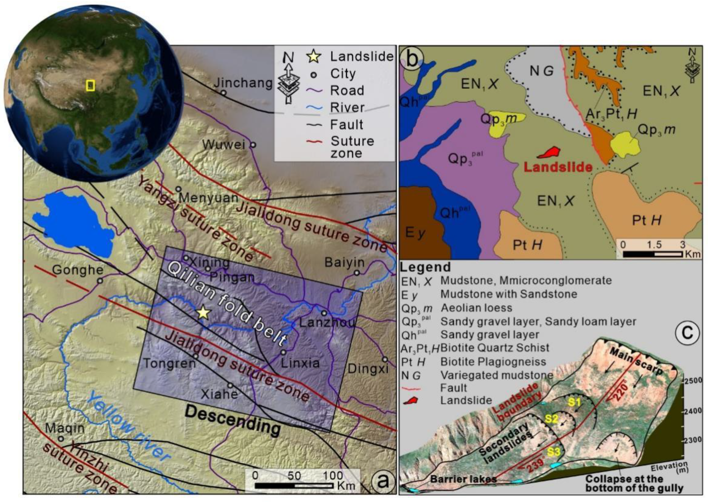
2. Study Area
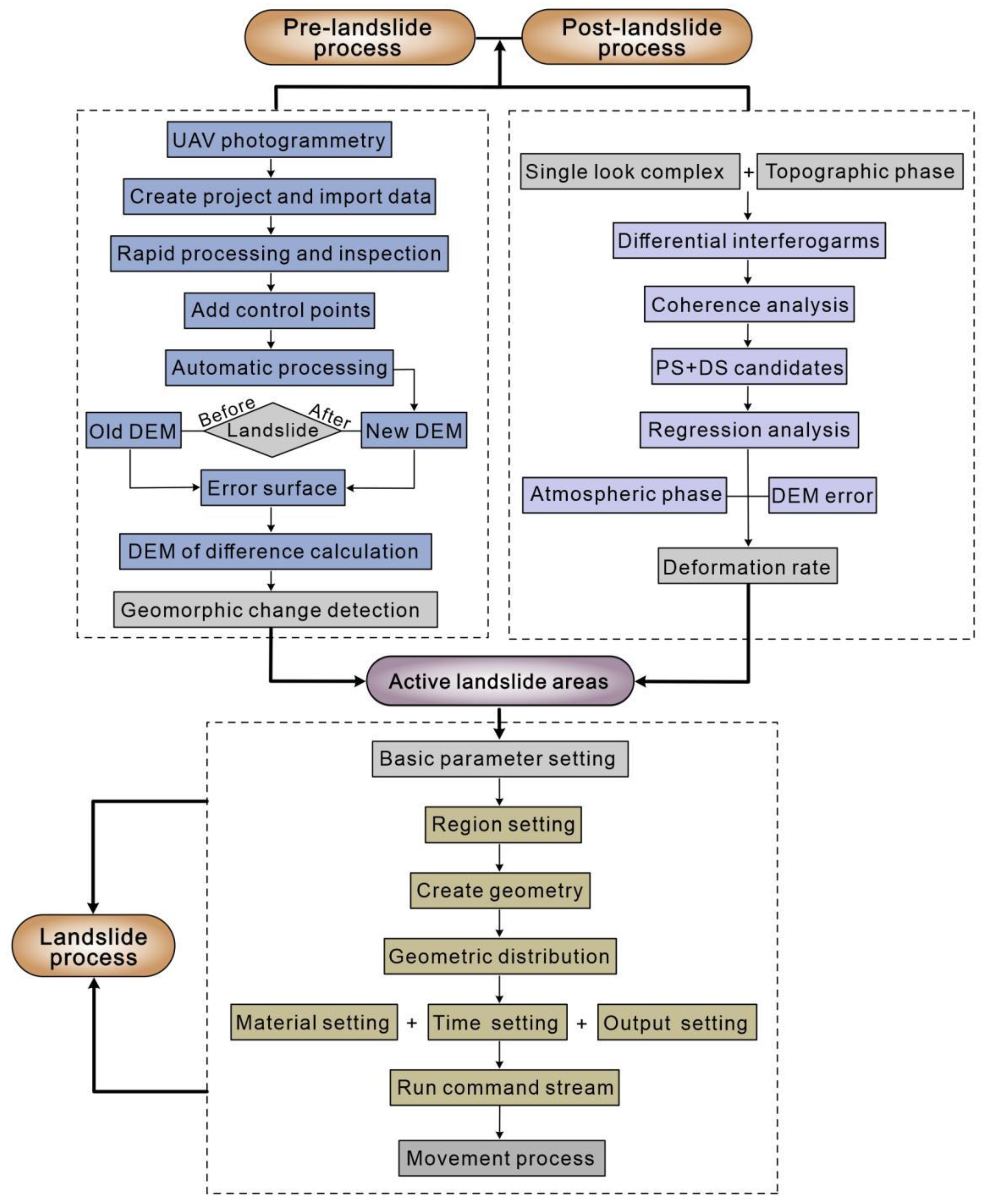
3. Methods and Data
3.1. Topographic Analysis
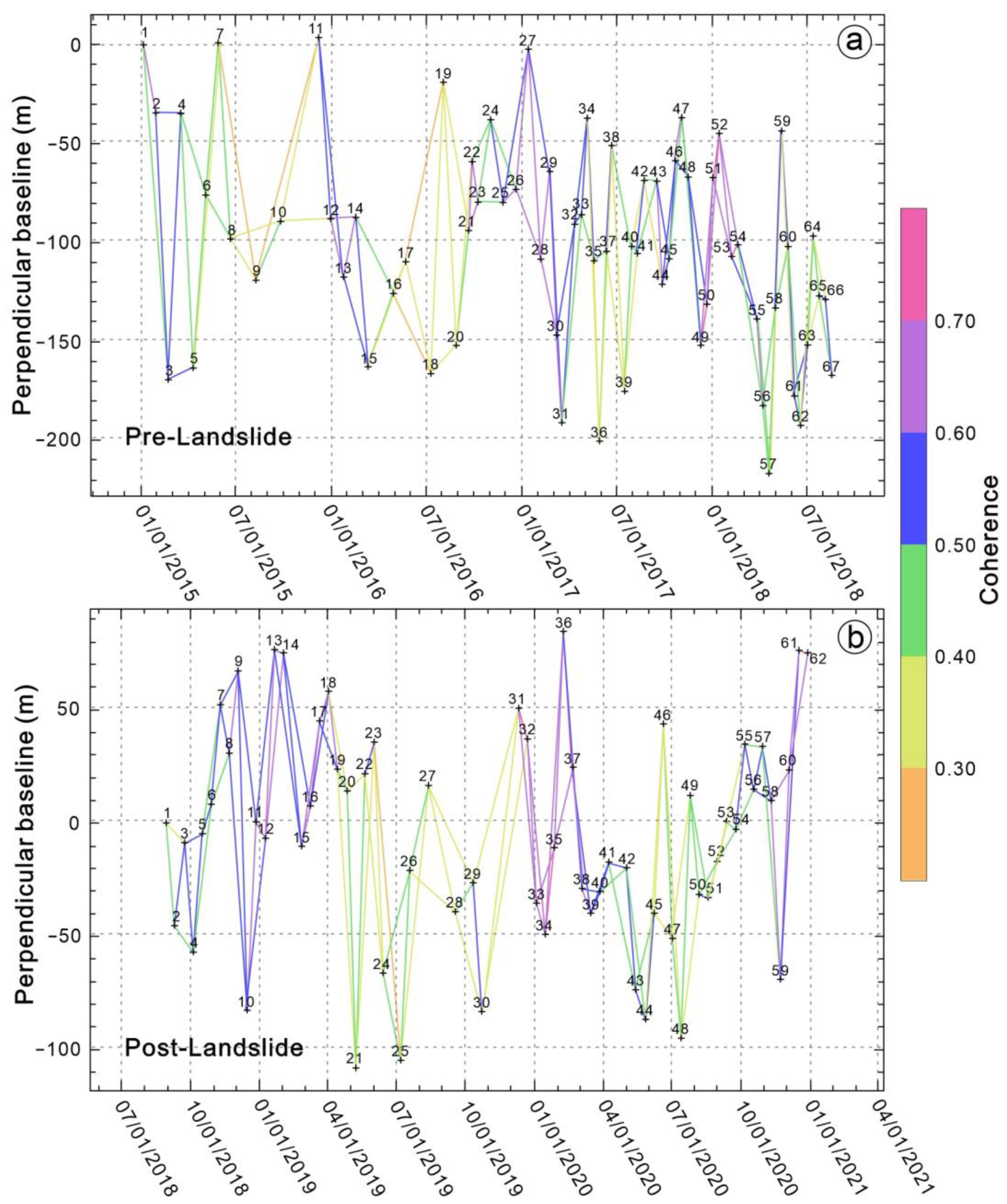
3.2. Multi-Temporal InSAR
3.3. Landslide Process Simulation
4. Results
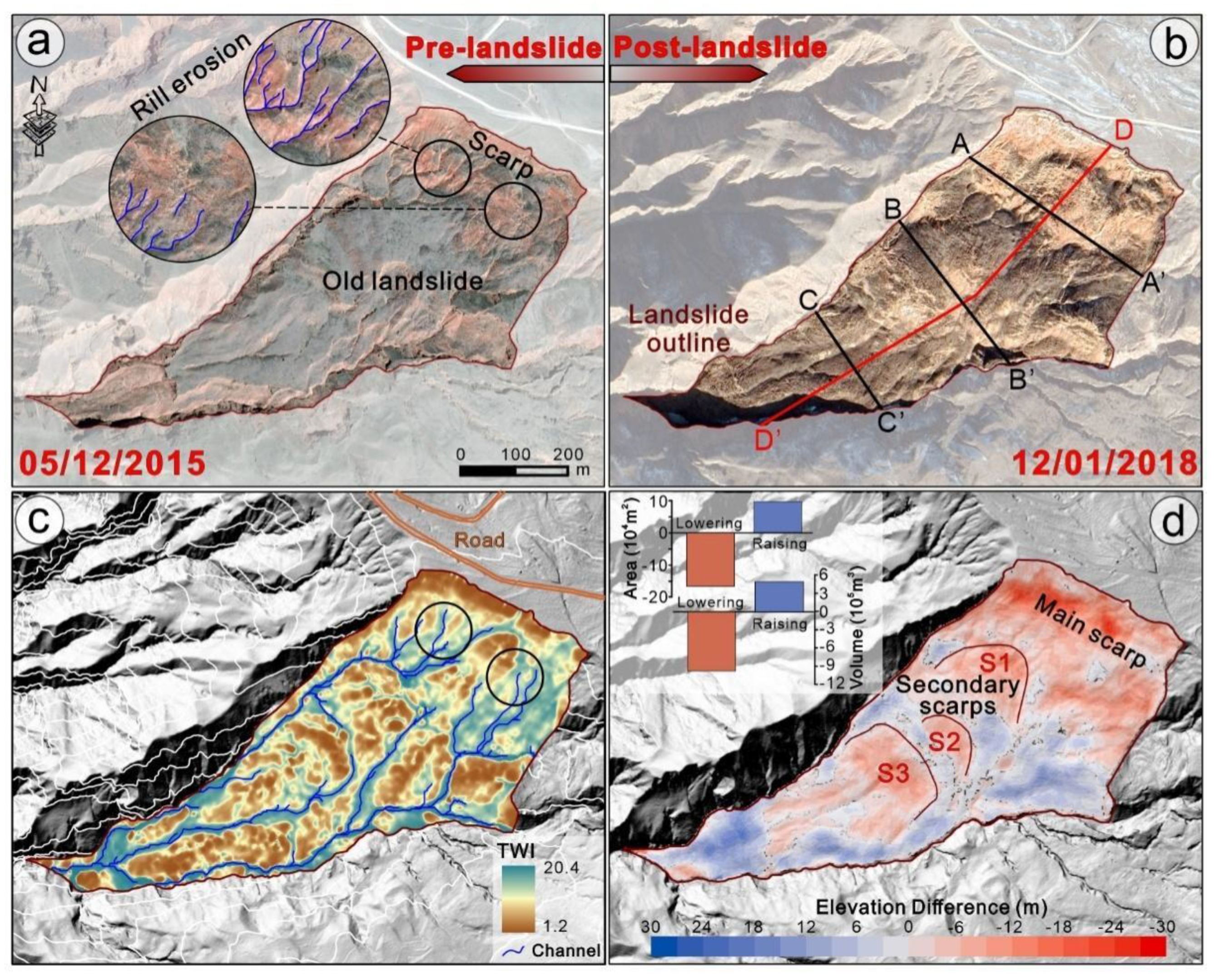
4.1. Topographic Changes before and after the Landslide
4.2. Deformation Evolution before and after the Landslide
4.3. Landslide Process Simulation
5. Discussion
5.1. Displacement Pattern of Rotational Landslide
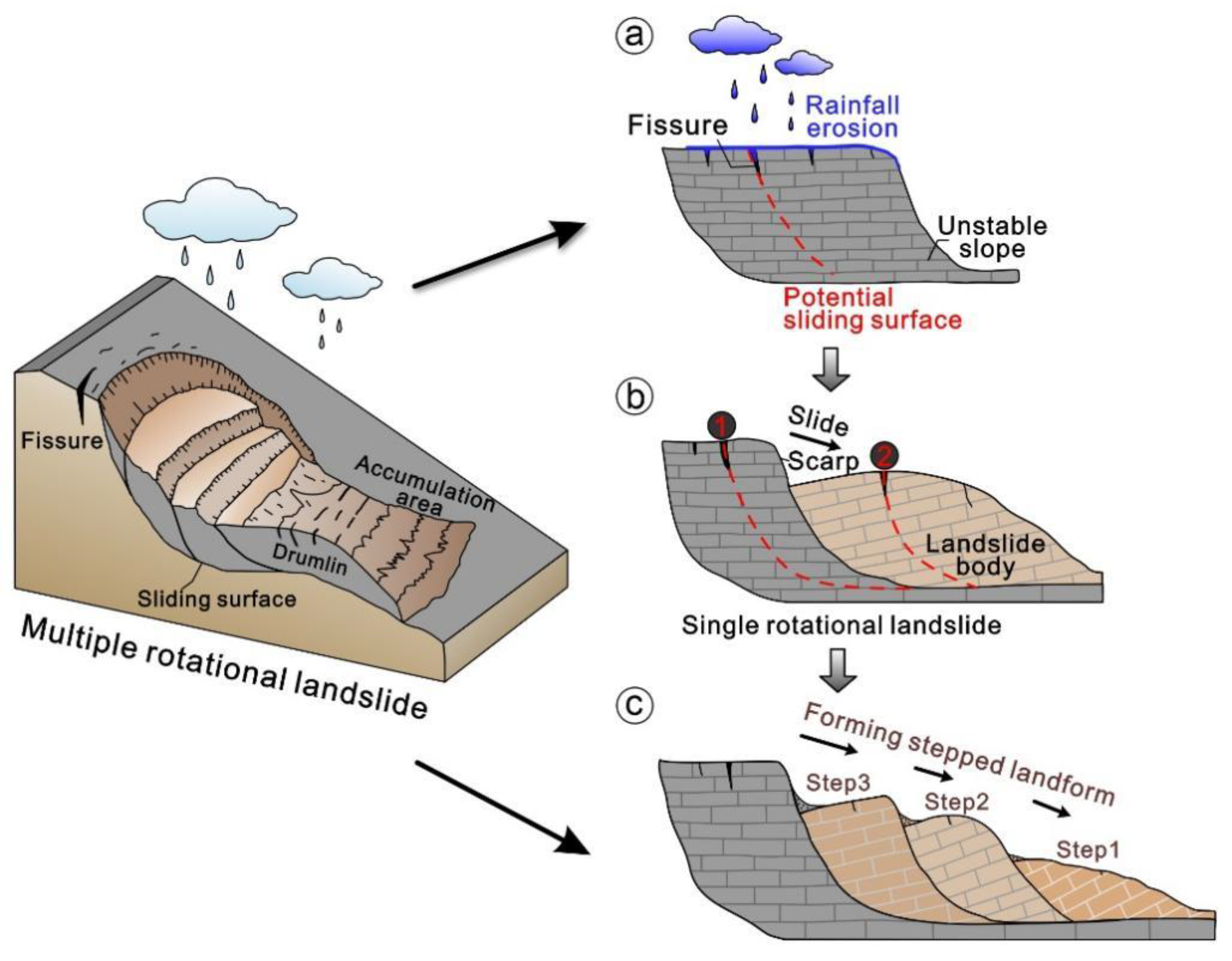
5.2. Evolution of Multiple Rotational Landslides
5.3. Inducing Factors of Landslide Reactivation
6. Conclusions
- (1)
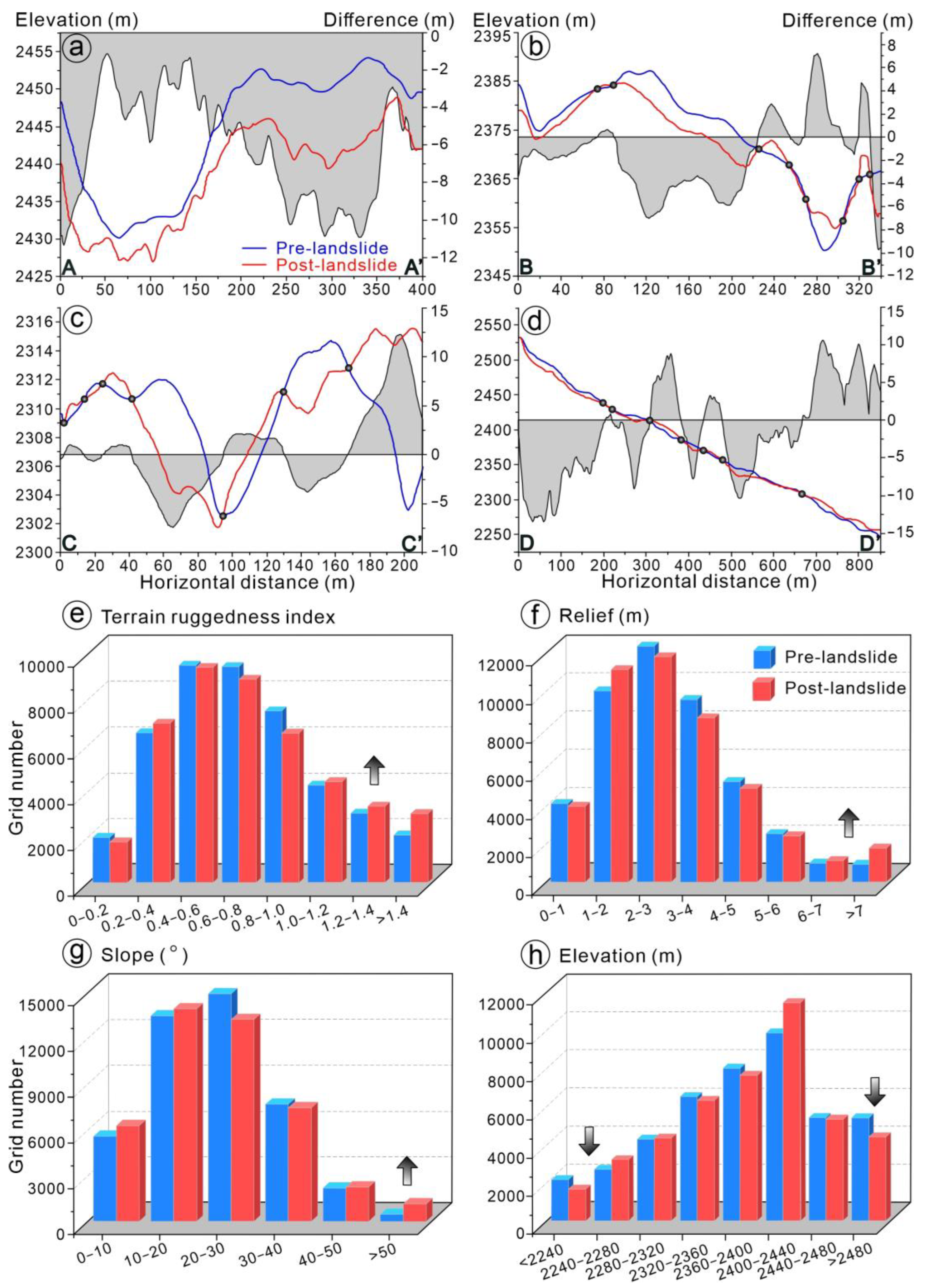
- The landslide changed the slope terrain. The changes are reflected in topographic factors, such as the terrain ruggedness index, relief, slope and elevation. The area and volume of the erosion areas are greater than those of the deposition areas for the main landslide. The percentage of surface lowering is 66% and that of surface raising is 34% by volume. The rill erosion, hydrological channels and TWI values indicate that the topographic changes in the landslide were affected by rainfall.
- (2)
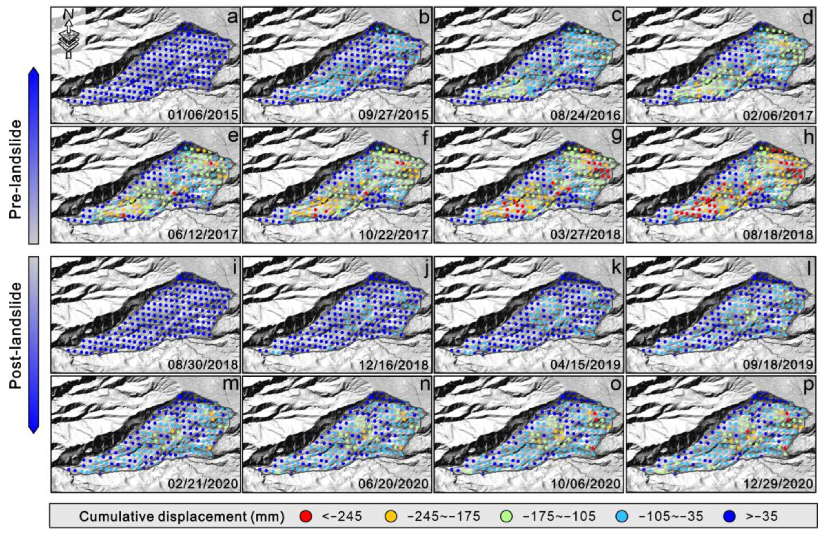
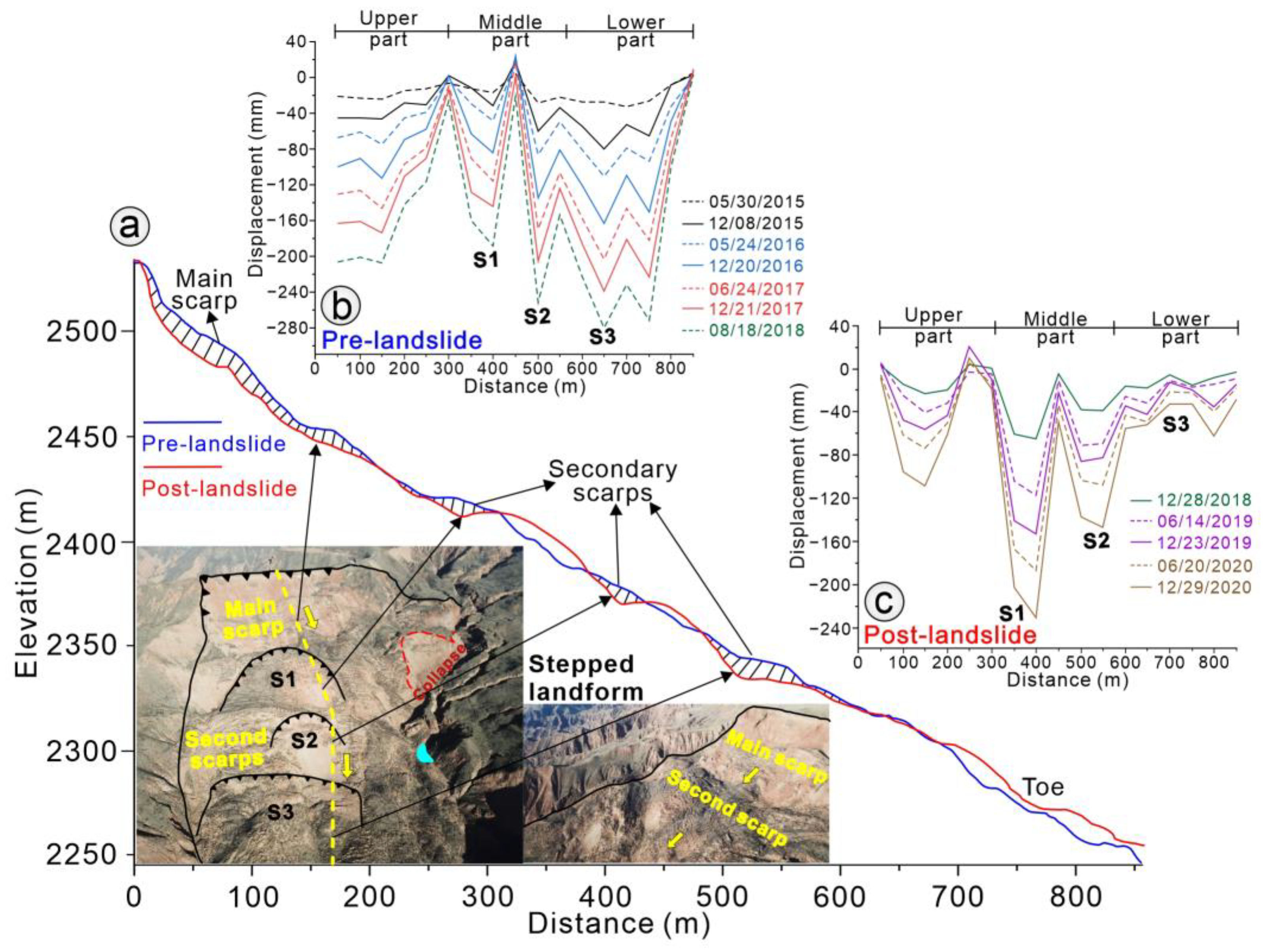
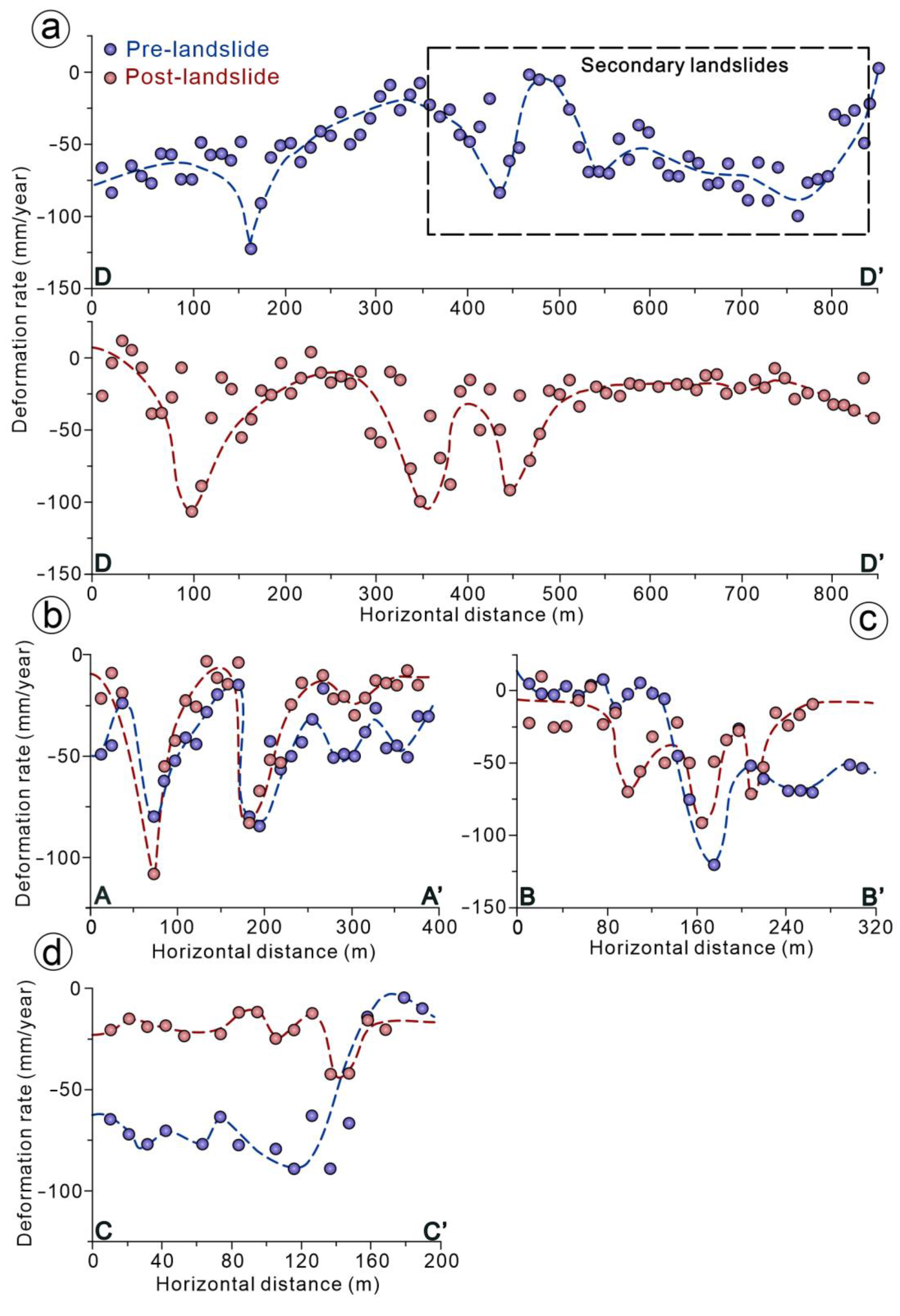
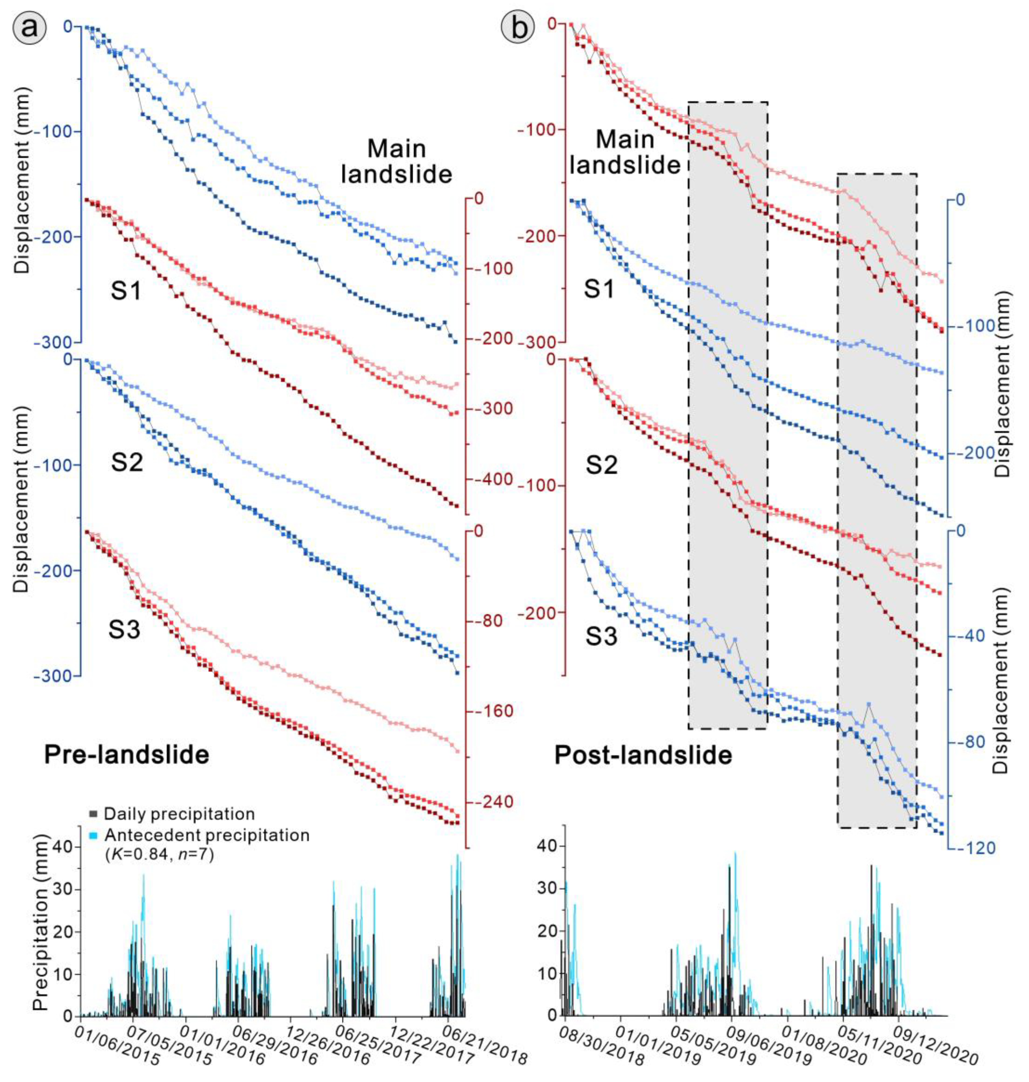
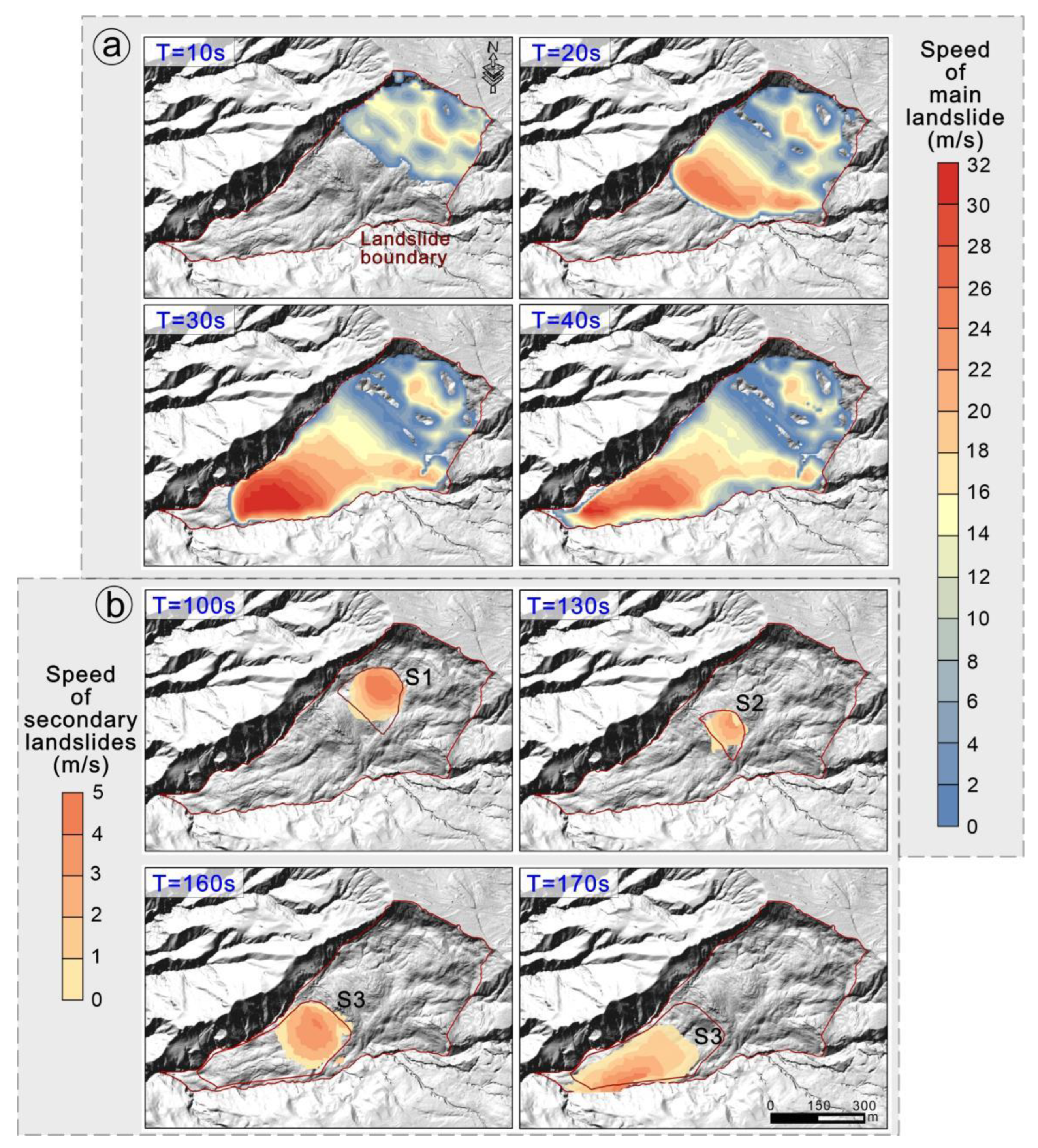
- The deformation before the landslide was mainly distributed in the scarp, middle and toe of the landslide. The cumulative displacement was mainly distributed from −175 to −306 mm. After the landslide, it was distributed in the eastern half of the scarp and the middle of the landslide. The maximum cumulative displacement was as high as −290 mm and −248 mm, respectively. Compared with the actual terrain, the variation in the displacement rate before and after the landslide was consistent with the topographic variation. The deformation areas in the middle of the landslide coincided with the secondary landslides. The cumulative displacement of the secondary landslide S1 after the landslide was as high as −231 mm.
- (3)
- Before the landslide, the displacement exhibited a linear trend. After the landslide, the displacement process showed alternating slow deformation stages and accelerated deformation stages. The accelerated deformation stages occurred during the rainy season in 2019 and 2020. Rainfall further accelerates the deformation rate of the landslide, thereby increasing the risk of reactivation.
- (4)
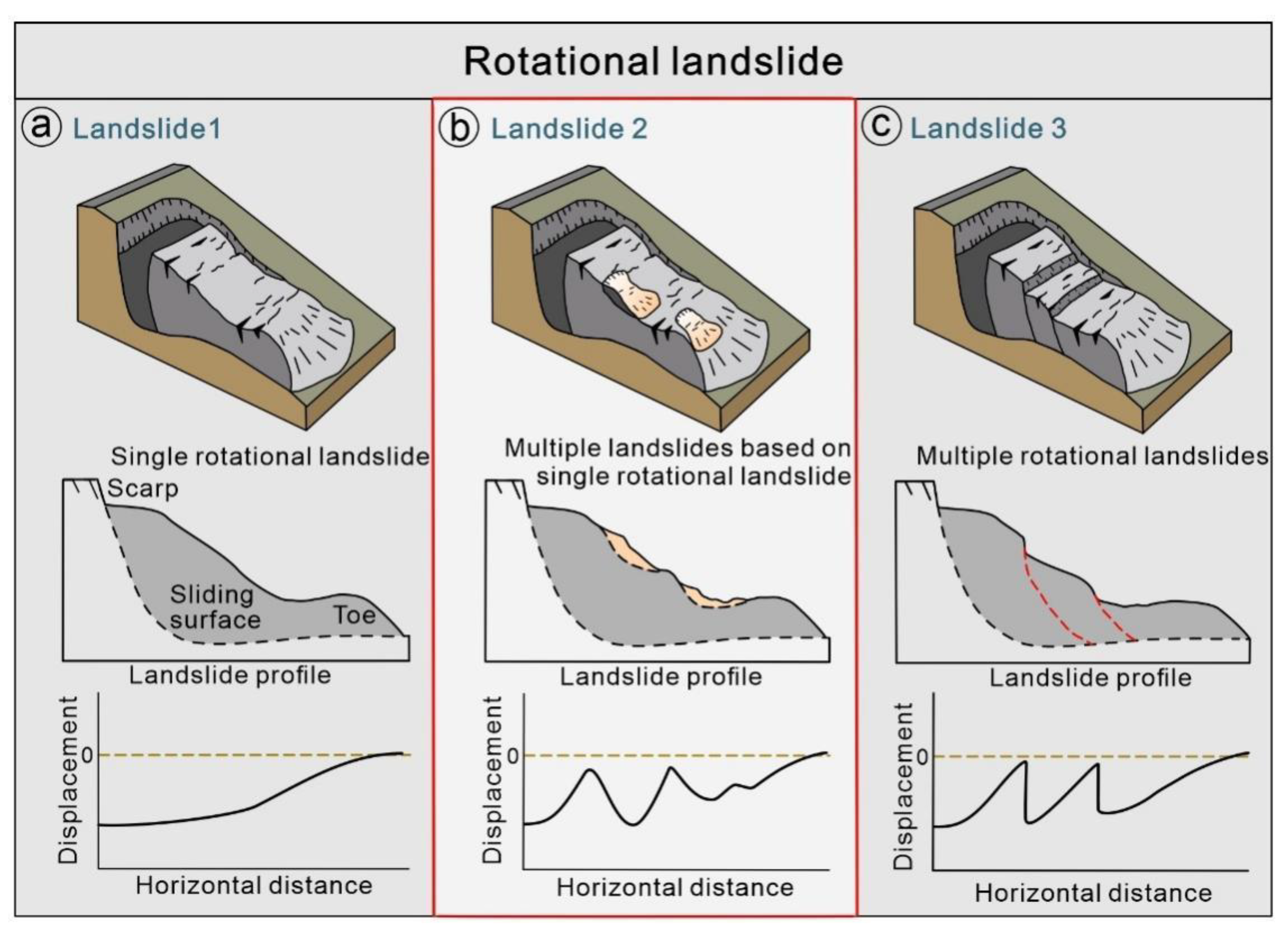
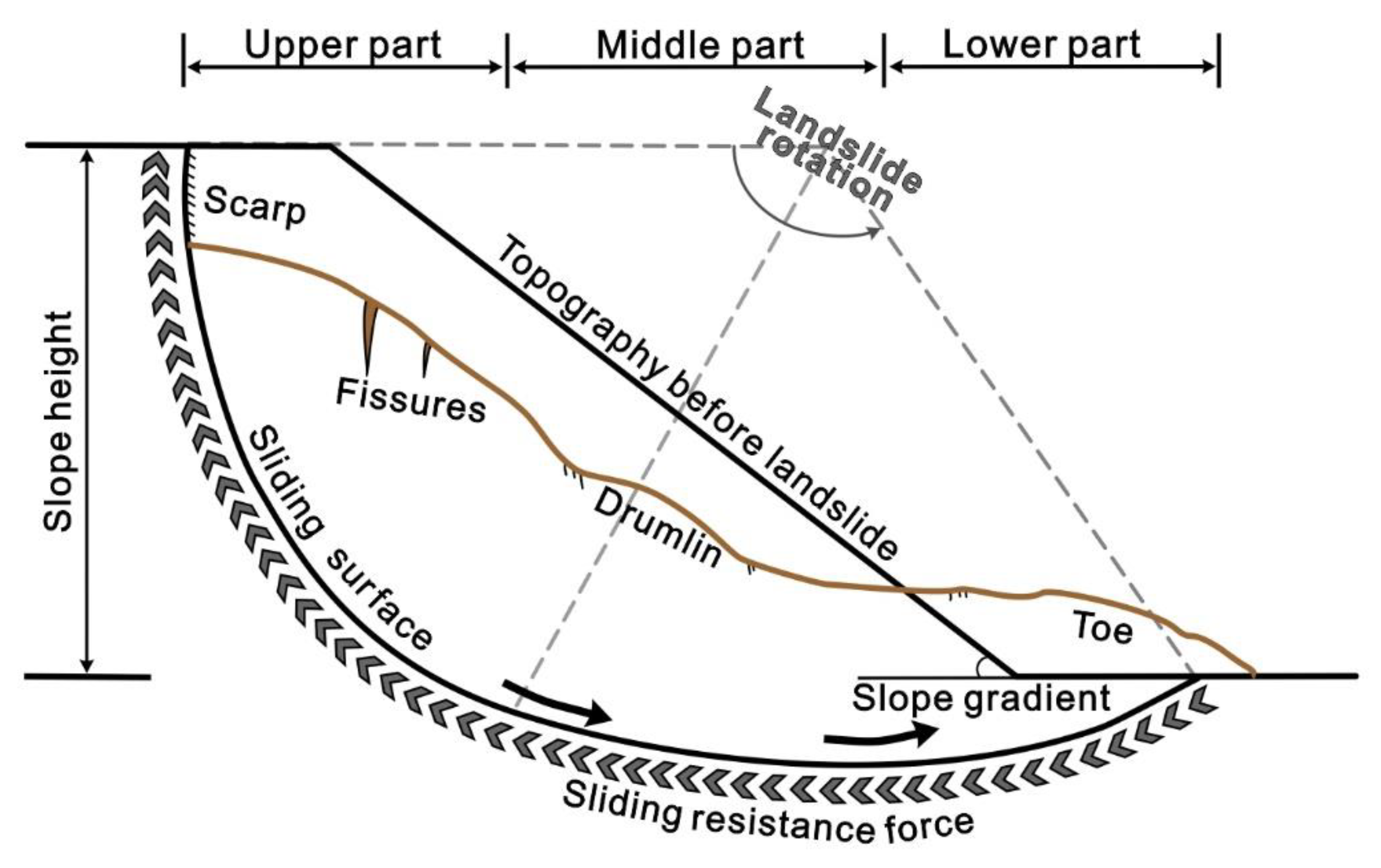
- The sliding surface forms a structural feature with a high and steep scarp, flat middle and slight warping of the leading edge. The difference of the sliding surface can generate different and complex displacement distributions. The displacement pattern conforms to that of multiple landslides based on a single rotational landslide.
Author Contributions
Funding
Data Availability Statement
Acknowledgments
Conflicts of Interest
References
- Barnes, P.M.; Lewis, K.B. Sheet slides and rotational failures on a convergent margin: The Kidnappers Slide, New Zealand. Sedimentology 1991, 38, 205–221. [Google Scholar] [CrossRef]
- Mather, A.E.; Griffiths, J.S.; Stokes, M. Anatomy of a “fossil” landslide from the Pleistocene of SE Spain. Geomorphology 2003, 50, 135–149. [Google Scholar] [CrossRef]
- Azanon, J.M.; Azor, A.; Perez-Pena, J.V.; Carrillo, J.M. Late Quaternary large-scale rotational slides induced by river incision: The Arroyo de Gor area (Guadix basin, SE Spain). Geomorphology 2005, 69, 152–168. [Google Scholar] [CrossRef]
- Li, B. Research on Formation Evolution Mechanism of Multiple Rotational Loess Landslides; Chang’an University: Xi’an, China, 2009. (In Chinese) [Google Scholar]
- Li, B.; Yin, Y.; Wu, S.; Shi, J. Failure mode and formation mechanism of multiple rotational loess landslides. J. Jilin Univ. 2012, 42, 760–769. [Google Scholar]
- Bromhead, E.N.; Ibsen, M.L. Bedding-controlled coastal landslides in Southeast Britain between Axmouth and the Thames Estuary. Landslides 2004, 1, 131–141. [Google Scholar] [CrossRef]
- Abascal, L.D.V.; Bonorino, G.G. Kinematics of a Translational/Rotational Landslide, Central Andes, Northwestern Argentina. Environ. Eng. Geosci. 2006, 12, 369–376. [Google Scholar] [CrossRef]
- Frattini, P.; Crosta, G.B.; Rossini, M.; Allievi, J. Activity and kinematic behaviour of deep-seated landslides from PS-InSAR displacement rate measurements. Landslides 2018, 15, 1053–1070. [Google Scholar] [CrossRef]
- Di Maio, C.; Vassallo, R.; Vallario, M. Plastic and viscous shear displacements of a deep and very slow landslide in stiff clay formation. Eng. Geol. 2013, 162, 53–66. [Google Scholar] [CrossRef]
- Yenes, M.; Monterrubio, S.; Nespereira, J.; Santos, G.; Fernandez-Macarro, B. Large landslides induced by fluvial incision in the Cenozoic Duero Basin (Spain). Geomorphology 2015, 246, 263–276. [Google Scholar] [CrossRef]
- Xin, P.; Liu, Z.; Wu, S.; Liang, C.; Lin, C. Rotational-translational landslides in the neogene basins at the northeast margin of the Tibetan Plateau. Eng. Geol. 2018, 244, 107–115. [Google Scholar] [CrossRef]
- Bayer, B.; Simoni, A.; Schmidt, D.; Bertello, L. Using advanced InSAR techniques to monitor landslide deformations induced by tunneling in the Northern Apennines, Italy. Eng. Geol. 2017, 226, 20–32. [Google Scholar] [CrossRef]
- Ma, S.; Qiu, H.; Hu, S.; Yang, D.; Liu, Z. Characteristics and geomorphology change detection analysis of the Jiangdingya landslide on July 12, 2018, China. Landslides 2021, 18, 383–396. [Google Scholar] [CrossRef]
- Jin, J.; Chen, G.; Meng, X.; Zhang, Y.; Shi, W.; Li, Y.; Yang, Y.; Jiang, W. Prediction of river damming susceptibility by landslides based on a logistic regression model and InSAR techniques: A case study of the Bailong River Basin, China. Eng. Geol. 2022, 299, 106562. [Google Scholar] [CrossRef]
- Keaton, J.R.; De Graff, J.V. Landslides: Investigation and Mitigation. Chapter 9—Surface Observation and Geologic Mapping; The National Academies of Sciences, Engineering, and Medicine: Washington, DC, USA, 1996; pp. 178–230. [Google Scholar]
- Bekaert, D.; Handwerger, A.L.; Agram, P.; Kirschbaum, D.B. InSAR-based detection method for mapping and monitoring slow-moving landslides in remote regions with steep and mountainous terrain: An application to Nepal. Remote Sens. Environ. 2020, 249, 111983. [Google Scholar] [CrossRef]
- Zapico, I.; Molina, A.; Laronne, J.B.; Castillo, L.S.; Duque, J.F.M. Stabilization by geomorphic reclamation of a rotational landslide in an abandoned mine next to the alto tajo natural park. Eng. Geol. 2020, 264, 105321. [Google Scholar] [CrossRef]
- Eker, R.; Aydın, A. Long-term retrospective investigation of a large, deep-seated, and slow-moving landslide using InSAR time series, historical aerial photographs, and UAV data: The case of Devrek landslide (NW Turkey). Catena 2021, 196, 104895. [Google Scholar] [CrossRef]
- Liu, Z.; Qiu, H.; Zhu, Y.; Liu, Y.; Yang, D.; Ma, S.; Zhang, J.; Wang, Y.; Wang, L.; Tang, B. Efficient Identification and Monitoring of Landslides by Time-Series InSAR Combining Single- and Multi-Look Phases. Remote Sens. 2022, 14, 1026. [Google Scholar] [CrossRef]
- Wang, L.; Qiu, H.; Zhou, W.; Zhu, Y.; Liu, Z.; Ma, S.; Yang, D.; Tang, B. The post-failure spatiotemporal deformation of certain translational landslides may follow the pre-failure pattern. Remote Sens. 2022, 14, 2333. [Google Scholar] [CrossRef]
- Niethammer, U.; James, M.R.; Rothmund, S.; Travelletti, J.; Joswig, M. UAV-based remote sensing of the Super-Sauze landslide: Evaluation and results. Eng. Geol. 2012, 128, 2–11. [Google Scholar] [CrossRef]
- Nappo, N.; Mavrouli, O.; Nex, F.; Westen, C.; Gambillara, R.; Michetti, A.M. Use of UAV-based photogrammetry products for semi-automatic detection and classification of asphalt road damage in landslide-affected areas. Eng. Geol. 2021, 294, 106363. [Google Scholar] [CrossRef]
- Tempa, K.; Peljor, K.; Wangdi, S.; Ghalley, R.; Jamtsho, K.; Ghalley, S.; Pradhan, P. UAV technique to localize landslide susceptibility and mitigation proposal: A case of Rinchending Goenpa landslide in Bhutan. Nat. Hazards Res. 2021, 1, 171–186. [Google Scholar] [CrossRef]
- Yang, D.; Qiu, H.; Hu, S.; Zhu, Y.; Cui, Y.; Du, C.; Liu, Z.; Pei, Y.; Cao, M. Spatiotemporal distribution and evolution characteristics of successive landslides on the Heifangtai tableland of the Chinese Loess Plateau. Geomorphology 2021, 378, 107619. [Google Scholar] [CrossRef]
- Godone, D.; Allasia, P.; Borrelli, L.; Gullà, G. UAV and Structure from Motion Approach to Monitor the Maierato Landslide Evolution. Remote Sens. 2020, 12, 1039. [Google Scholar] [CrossRef] [Green Version]
- Kyriou, A.; Nikolakopoulos, K.; Koukouvelas, I.; Lampropoulou, P. Repeated UAV Campaigns, GNSS Measurements, GIS, and Petrographic Analyses for Landslide Mapping and Monitoring. Minerals 2021, 11, 300. [Google Scholar] [CrossRef]
- Colesanti, C.; Wasowski, J. Investigating landslides with space-borne synthetic aperture radar (SAR) interferometry. Eng. Geol. 2006, 88, 173–199. [Google Scholar] [CrossRef]
- Squarzoni, G.; Bayer, B.; Franceschini, S.; Simoni, A. Pre and post failure dynamics of landslides in the northern apennines revealed by space-borne synthetic aperture radar interferometry (insar). Geomorphology 2020, 369, 107353. [Google Scholar] [CrossRef]
- Zhu, Y.; Qiu, H.; Yang, D.; Liu, Z.; Ma, S.; Pei, Y.; He, J.; Du, C.; Sun, H. Pre- and post-failure spatiotemporal evolution of loess landslides: A case study of the jiangou landslide in ledu, china. Landslides 2021, 18, 3475–3484. [Google Scholar] [CrossRef]
- Bian, S.; Chen, G.; Zeng, R.; Meng, X.; Jin, J.; Lin, L.; Zhang, Y.; Shi, W. Post-failure evolution analysis of an irrigation-induced loess landslide using multiple remote sensing approaches integrated with time-lapse ERT imaging: Lessons from Heifangtai, China. Landslides 2022, 19, 1179–1197. [Google Scholar] [CrossRef]
- Petley, D.N.; Bulmer, M.H.; Murphy, W. Patterns of movement in rotational and translational landslides. Geology 2002, 30, 719–722. [Google Scholar] [CrossRef]
- Schlögel, R.; Doubre, C.; Malet, J.P.; Masson, F. Landslide deformation monitoring with ALOS/PALSAR imagery: A D-InSAR geomorphological interpretation method. Geomorphology 2015, 231, 314–330. [Google Scholar] [CrossRef]
- Chen, K.T.; Wu, J.H. Simulating the failure process of the Xinmo landslide using discontinuous deformation analysis. Eng. Geol. 2018, 239, 269–281. [Google Scholar] [CrossRef]
- Yan, Y.; Cui, Y.; Guo, J.; Hu, S.; Wang, Z.; Yin, S. Landslide reconstruction using seismic signal characteristics and numerical simulations: Case study of the 2017 “6.24” Xinmo landslide. Eng. Geol. 2020, 270, 105582. [Google Scholar] [CrossRef]
- Quecedo, M.; Pastor, M.; Herreros, M.I.; Fernández Merodo, J.A. Numerical modelling of the propagation of fast landslides using the finite element method. Int. J. Numer. Methods Eng. 2004, 59, 755–794. [Google Scholar] [CrossRef]
- Pirulli, M.; Scavia, C.; Tararbra, M. On the Use of Numerical Models for Flow-like Landslide Simulation. Eng. Geol. Soc. Territ. 2015, 2, 1625–1638. [Google Scholar]
- Ouyang, C.; Zhou, K.; Xu, Q.; Yin, J.; Peng, D.; Wang, D.; Li, W. Dynamic analysis and numerical modeling of the 2015 catastrophic landslide of the construction waste landfill at guangming, shenzhen, china. Landslides 2017, 14, 705–718. [Google Scholar] [CrossRef]
- An, H.; Ouyang, C.; Zhou, S. Dynamic process analysis of the Baige landslide by the combination of DEM and long-period seismic waves. Landslides 2021, 18, 1625–1639. [Google Scholar] [CrossRef]
- Fan, X.; Yang, F.; Subramanian, S.; Xu, Q.; Feng, Z.; Mavrouli, O.; Peng, M.; Ouyang, C.; Jansen, J.; Huang, R. Prediction of a multi-hazard chain by an integrated numerical simulation approach: The Baige landslide, Jinsha River, China. Landslides 2020, 17, 147–164. [Google Scholar] [CrossRef]
- Zhou, Q.; Xu, Q.; Zhou, S.; Peng, D.; Zhou, X.; Qi, X. Movement process of abrupt loess flowslide based on numerical simulation-a case study of Chenjia 8# on the Heifangtai Terrace. Mt. Res. 2019, 37, 528–537. [Google Scholar]
- Ouyang, C.; An, H.; Zhou, S.; Wang, Z.; Su, P.; Wang, D.; Cheng, D.; She, J. Insights from the failure and dynamic characteristics of two sequential landslides at Baige village along the Jinsha River, China. Landslides 2019, 16, 1397–1414. [Google Scholar] [CrossRef]
- Ma, P.; Cui, Y.; Wang, W.; Lin, H.; Zhang, Y. Coupling InSAR and numerical modeling for characterizing landslide movements under complex loads in urbanized hillslopes. Landslides 2021, 18, 1611–1623. [Google Scholar] [CrossRef]
- Roy, P.; Martha, T.R.; Khanna, K.; Jain, N.; Kumar, K.V. Time and path prediction of landslides using insar and flow model. Remote Sens. Environ. 2022, 271, 112899. [Google Scholar] [CrossRef]
- Wheaton, J.M. Trends and challenges in geomorphic change detection. In Proceedings of the Australia and New Zealand Geomorphology Group Annual Conference, Mount Tamborine, Australia, 3 December 2014. [Google Scholar]
- GCD. Geomorphic Change Detection Software, Version 7. Available online: https://gcd.riverscapes.net/ (accessed on 1 October 2022).
- Hu, S.; Qiu, H.; Wang, N.; Wang, X.; Ma, S.; Yang, D.; Wei, N.; Liu, Z.; Shen, Y.; Cao, M.; et al. Movement process, geomorphological changes, and influencing factors of a reactivated loess landslide on the right bank of the middle of the Yellow River, China. Landslides 2022, 19, 1265–1295. [Google Scholar] [CrossRef]
- Ferretti, A.; Fumagalli, A.; Novali, F.; Prati, C.; Rocca, F.; Rucci, A. A New Algorithm for Processing Interferometric Data-Stacks: SqueeSAR. IEEE Trans. Geosci. Remote Sens. 2011, 49, 3460–3470. [Google Scholar] [CrossRef]
- Shi, X.; Xu, J.; Jiang, H.; Zhang, L.; Liao, M. Slope stability state monitoring and updating of the Outang landslide, Three Gorges Area with time series InSAR analysis. Earth Sci. 2019, 44, 4284–4292. [Google Scholar]
- Wasowski, J.; Bovenga, F. Investigating landslides and unstable slopes with satellite Multi Temporal Interferometry: Current issues and future perspectives. Eng. Geol. 2014, 174, 103–138. [Google Scholar] [CrossRef]
- Dong, J.; Zhang, L.; Tang, M.; Liao, M.; Xu, Q.; Gong, J.; Ao, M. Mapping landslide surface displacements with time series SAR interferometry by combining persistent and distributed scatterers: A case study of Jiaju landslide in Danba, China. Remote Sens. Environ. 2018, 205, 180–198. [Google Scholar] [CrossRef]
- Zhang, Z.; Wang, C.; Tang, Y.; Fu, Q.; Zhang, H. Subsidence monitoring in coal area using time-series InSAR combining persistent scatterers and distributed scatterers. Int. J. Appl. Earth Obs. Geoinf. 2015, 39, 49–55. [Google Scholar] [CrossRef]
- Liu, G.; Chen, Q.; Luo, X.; Cai, G. Principle and Application of Insar; China Science Publishing Group: Beijing, China, 2019; pp. 80–81. (In Chinese) [Google Scholar]
- Zêzere, J.L.; Trigo, R.M.; Trigo, I.F. Shallow and deep landslides induced by rainfall inthe Lisbon region (Portugal): Assessment of relationships with the North Atlantic Oscillation. Nat. Hazards Earth Syst. Sci. 2005, 5, 331–344. [Google Scholar] [CrossRef]
- Guo, X.; Cui, P.; Li, Y. Debris Flow Warning Threshold Based on Antecedent Rainfall: A Case Study in Jiangjia Ravine, Yunnan, China. J. Mt. Sci. 2013, 10, 305–314. [Google Scholar] [CrossRef]
- Horton, A.J.; Hales, T.C.; Ouyang, C.; Fan, X. Identifying post-earthquake debris flow hazard using Massflow. Eng. Geol. 2019, 258, 105134. [Google Scholar] [CrossRef]
- Zeng, P.; Sun, X.; Xu, Q.; Li, T.; Zhang, T. 3D probabilistic landslide run-out hazard evaluation for quantitative risk assessment purposes. Eng. Geol. 2021, 293, 106303. [Google Scholar] [CrossRef]
- Liu, N. Research on the Stability of Loess Landslide in Xinyuan Xining; Tianjin Chengjian University: Tianjin, China, 2013. (In Chinese) [Google Scholar]
- Xin, P.; Wang, T.; Wu, S. The formation mechanism of multilevel rotational mudstone landslides in Hanjiashan of Datong County, Qinghai Province. Acta Geosci. Sin. 2015, 36, 771–780. [Google Scholar]
- Cao, P. Formation Mechanism and Stability of Baige Landslide in Eastern Qinghai-Tibet Plateau; Kunming University of Science and Technology: Kunming, China, 2020. (In Chinese) [Google Scholar]
- Livio, F.A.; Zerboni, A.; Ferrario, M.F.; Mariani, G.S.; Martinelli, E.; Amit, R. Triggering processes of deep-seated gravitational slope deformation (DSGSD) in an un-glaciated area of the Cavargna Valley (Central Southern Alps) during the Middle Holocene. Landslides 2022, 19, 1825–1841. [Google Scholar] [CrossRef]
- Vick, L.M.; Böhme, M.; Rouyet, L.; Bergh, S.G.; Corner, G.D.; Lauknes, T.R. Structurally controlled rock slope deformation in northern Norway. Landslides 2020, 17, 1745–1776. [Google Scholar]
- Du, Y.; Yan, E.; Cai, J.; Gao, X.; Liu, W. Mechanical discrimination on stability state of progressive failure of broken-line complex landslides. Chin. J. Geotech. Eng. 2022, 11, 3–8. [Google Scholar]
- Li, S.; Li, C.; Yao, D.; Liu, C.; Zhang, Y. Multiscale nonlinear analysis of failure mechanism of loess-mudstone landslide. Catena 2022, 213, 106188. [Google Scholar] [CrossRef]
- Singeisen, C.; Massey, C.; Wolter, A.; Kellett, R.; Bloom, C.; Stahl, T.; Gasston, C.; Jones, K. Mechanisms of rock slope failures triggered by the 2016 Mw 7.8 Kaikōura earthquake and implications for landslide susceptibility. Geomorphology 2022, 415, 108386. [Google Scholar] [CrossRef]
- Du, Y.; Yan, E.; Cai, J.; Zhou, Y.; Wang, J. A mechanical model of progressive failure of linear complex landslides. Chin. J. Rock Mech. Eng. 2021, 40, 490–502. [Google Scholar]
- Pánek, T.; Šilhán, K.; Hradecký, J.; Strom, A.; Smolková, V.; Zerkal, O. A megalandslide in the Northern Caucasus foredeep (Uspenskoye, Russia): Geomorphology, possible mechanism and age constraints. Geomorphology 2012, 177–178, 144–157. [Google Scholar] [CrossRef]
- Pei, Y.; Qiu, H.; Yang, D.; Liu, Z.; Ma, S.; Li, J.; Cao, M.; Wufuer, W. Increasing landslide activity in the Taxkorgan River Basin (eastern Pamirs Plateau, China) driven by climate change. CATENA 2023, 223, 106911. [Google Scholar] [CrossRef]
- Zhou, W.; Qiu, H.; Wang, L.; Pei, Y.; Tang, B.; Ma, S.; Yang, D.; Cao, M. Combining rainfall-induced shallow landslides and subsequent debris flows for hazard chain prediction. CATENA 2022, 213, 106199. [Google Scholar] [CrossRef]
- Qiu, H.; Zhu, Y.; Zhou, W.; Sun, H.; He, J.; Liu, Z. Influence of DEM resolution on landslide simulation performance based on the Scoops3D model. Geomat. Nat. Hazards Risk 2022, 13, 1663–1681. [Google Scholar] [CrossRef]
- Xie, J.; Uchimura, T.; Wang, G.; Selvarajah, H.; Maqsood, Z.; Shen, Q.; Mei, G.; Qiao, S. Predicting the sliding behavior of rotational landslides based on the tilting measurement of the slope surface. Eng. Geol. 2020, 269, 105554. [Google Scholar] [CrossRef]
- Massey, C.I.; Petley, D.N.; McSaveney, M.J. Patterns of movement in reactivated landslides. Eng. Geol. 2013, 159, 1–19. [Google Scholar] [CrossRef]
- Zhang, S.; Lin, H.; Chen, Y.; Wang, Y.; Zhao, Y. Acoustic emission and failure characteristics of cracked rock under freezing-thawing and shearing. Theor. Appl. Fract. Mech. 2022, 121, 103537. [Google Scholar] [CrossRef]
- Stumpf, A.; Malet, J.P.; Kerle, N.; Niethammer, U.; Rothmund, S. Image-based mapping of surface fissures for the investigation of landslide dynamics. Geomorphology 2013, 186, 12–27. [Google Scholar] [CrossRef] [Green Version]
- Rosone, M.; Ziccarelli, M.; Ferrari, A.; Farulla, C.A. On the reactivation of a large landslide induced by rainfall in highly fissured clays. Eng. Geol. 2018, 235, 20–38. [Google Scholar] [CrossRef]
- Ma, S.; Qiu, H.; Yang, D.; Wang, J.; Zhu, Y.; Tang, B.; Sun, K.; Cao, M. Surface multi-hazard effect of underground coal mining. Landslides 2022, 20, 39–52. [Google Scholar] [CrossRef]


| Topographic Parameters | Main Lanslide | Secondary Landslide S1 | Secondary Landslide S2 | Secondary Landslide S3 |
|---|---|---|---|---|
| Perimeter (m) | 2749 | 784 | 521 | 1174 |
| Area (m2) | 276,646 | 31,079 | 15,068 | 69,416 |
| Maximum length (m) | 886 | 172 | 109 | 432 |
| Maximum width (m) | 490 | 208 | 195 | 215 |
| L/W ratio | 1.81 | 0.83 | 0.56 | 2.01 |
| Average slope (°) | 23.49 | 19.83 | 21.02 | 20.44 |
| Plane morphology | Tongue shape | Semicircle shape | Semicircle shape | Tongue shape |
| Landslide | Parameters | Surface Lowering | Surface Raising |
|---|---|---|---|
| Main lanslide | Area (m2) | 168,013 | 97,350 |
| Volume (m3) | 971,383 ±33,602 | 492,059 ±19,470 | |
| Thickness (m) | 5.78 ±0.20 | 5.05 ±0.20 | |
| Secondary landslide S1 | Area (m2) | 21,575 | 7563 |
| Volume (m3) | 119,116 ±4315 | 28,707 ±1512 | |
| Thickness (m) | 5.52 ±0.20 | 3.80 ±0.20 | |
| Secondary landslide S2 | Area (m2) | 8431 | 5125 |
| Volume (m3) | 31,069 ±1686 | 10,100 ±1025 | |
| Thickness (m) | 3.68 ±0.20 | 1.97 ±0.20 | |
| Secondary landslide S3 | Area (m2) | 37,144 | 28,825 |
| Volume (m3) | 163,751 ±7429 | 220,502 ±5765 | |
| Thickness (m) | 4.41 ±0.20 | 7.65 ±0.20 |
Disclaimer/Publisher’s Note: The statements, opinions and data contained in all publications are solely those of the individual author(s) and contributor(s) and not of MDPI and/or the editor(s). MDPI and/or the editor(s) disclaim responsibility for any injury to people or property resulting from any ideas, methods, instructions or products referred to in the content. |
© 2023 by the authors. Licensee MDPI, Basel, Switzerland. This article is an open access article distributed under the terms and conditions of the Creative Commons Attribution (CC BY) license (https://creativecommons.org/licenses/by/4.0/).
Share and Cite
Ma, S.; Qiu, H.; Zhu, Y.; Yang, D.; Tang, B.; Wang, D.; Wang, L.; Cao, M. Topographic Changes, Surface Deformation and Movement Process before, during and after a Rotational Landslide. Remote Sens. 2023, 15, 662. https://doi.org/10.3390/rs15030662
Ma S, Qiu H, Zhu Y, Yang D, Tang B, Wang D, Wang L, Cao M. Topographic Changes, Surface Deformation and Movement Process before, during and after a Rotational Landslide. Remote Sensing. 2023; 15(3):662. https://doi.org/10.3390/rs15030662
Chicago/Turabian StyleMa, Shuyue, Haijun Qiu, Yaru Zhu, Dongdong Yang, Bingzhe Tang, Daozheng Wang, Luyao Wang, and Mingming Cao. 2023. "Topographic Changes, Surface Deformation and Movement Process before, during and after a Rotational Landslide" Remote Sensing 15, no. 3: 662. https://doi.org/10.3390/rs15030662