Article

Vertically Resolved Global Ocean Light Models Using Machine Learning

by
Pannimpullath Remanan Renosh
*,
Jie Zhang
,
Raphaëlle Sauzède
and
Hervé Claustre
Laboratoire d’Océanographie de Villefranche, Institut de la Mer de Villefranche, Sorbonne Université, CNRS INSU, 06230 Villefranche-sur-Mer, France
*
Author to whom correspondence should be addressed.
Remote Sens. 2023, 15(24), 5663; https://doi.org/10.3390/rs15245663
Submission received: 22 September 2023 / Revised: 30 November 2023 / Accepted: 3 December 2023 / Published: 7 December 2023
(This article belongs to the Special Issue AI for Marine, Ocean and Climate Change Monitoring)

Abstract

:
The vertical distribution of light and its spectral composition are critical factors influencing numerous physical, chemical, and biological processes within the oceanic water column. In this study, we present vertically resolved models of downwelling irradiance (ED) at three different wavelengths and photosynthetically available radiation (PAR) on a global scale. These models rely on the SOCA (Satellite Ocean Color merged with Argo data to infer bio-optical properties to depth) methodology, which is based on an artificial neural network (ANN). The new light models are trained with light profiles (ED/PAR) acquired from BioGeoChemical-Argo (BGC-Argo) floats. The model inputs consist of surface ocean color radiometry data (i.e., R r s , PAR, and k d ( 490 ) ) derived by satellite and extracted from the GlobColour database, temperature and salinity profiles originating from BGC-Argo, as well as temporal components (day of the year and local time in cyclic transformation). The model outputs correspond to ED profiles at the three wavelengths of the BGC-Argo measurements (i.e., 380, 412, and 490 nm) and PAR profiles. We assessed the retrieval of light profiles by these light models using three different datasets: BGC-Argo profiles that were not used for the training (i.e., 20% of the initial database); data from four independent BGC-Argo floats that were used neither for the training nor for the 20% validation dataset; and the SeaBASS database (in situ data collected from various oceanic cruises). The light models show satisfactory predictions when thus compared with real measurements. From the 20% validation database, the light models retrieve light variables with high accuracies (root mean squared error (RMSE)) of 76.42 μmol quanta m−2 s−1 for PAR and 0.04, 0.08, and 0.09 W m−2 nm−1 for ED380, ED412, and ED490, respectively. This corresponds to a median absolute percent error (MAPE) that ranges from 37% for ED490 and PAR to 39% for ED380 and ED412. The estimated accuracy metrics across these three validation datasets are consistent and demonstrate the robustness and suitability of these light models for diverse global ocean applications.

1. Introduction

Incoming solar radiation, 40% of which originates from the visible part of the spectrum, stands as the main source of energy for the entire Earth system. In the ocean, this radiation propagates and attenuates from the surface to the depths. The characterization of this propagation critically depends on accurate estimation of the downwelling irradiance, ED (W m 2 ), over various depths. This estimation serves as the core for understanding numerous surface and sub-surface oceanic processes, as well as for the quantification of key oceanic variables.
More specifically, knowledge of ED at different depths is crucial for the quantification of various photo-dependent processes, such as oceanic phytoplankton photosynthesis [1,2], which relies on photosynthetically available radiation (PAR) as an indication of the integration of irradiance over the visible domain (400–700 nm). Additionally, knowledge of ED is essential for determining the heating rate of the upper ocean [3,4], involving the entire spectrum from UV to infrared, and also for the photo-production or destruction of organic molecules [5], often driven by the energetic UV part of the spectrum.
The derivative of the ED with respect to depth, known as the diffuse attenuation coefficient, k d (m 1 ), is a reliable parameter that can be related to specific optically significant substances, such as chlorophyll-a concentration (Chla), the proxy for phytoplankton biomass [6,7] or colored dissolved organic matter (CDOM) [8], the proxy for dissolved organic carbon (DOC) [9].
For the computation of remote sensing reflectance ( R r s ), in situ measurements of ED and upwelling irradiance (LU), which measure the radiant flux per unit area per unit solid angle (W m 2 sr 1 ), are essential. R r s , linked to the concentration of optically significant substances and accessible from satellite observations, is an apparent optical property (AOP) of fundamental importance in ocean-color-related science. Notably, ocean color products, including R r s , as well as ocean surface heat flux, are labeled as essential oceanic variables within the framework of the Global Ocean Observation System (GOOS) program.
Most of the irradiance (multi- or hyper-spectral, PAR) profiles acquired so far essentially result from the deployment of irradiance profilers from ships. These measurements (and the subsequent derivation of k d ), along with the concurrent measurements of key biogeochemical variables (e.g., Chla) [10,11,12], have contributed to the establishment of reference databases. These databases have become the key for assessing the bio-optical and trophic status of oceanic environments [12,13] as well as supporting validation activities for satellite ocean color radiometric products [14].
The implementation of the BioGeoChemical(BGC)-Argo program, of which irradiance is one of the six core variables, has opened up a revolutionary way to acquire numerous irradiance profiles and develop internally consistent databases [15,16]. In particular, long time series are now available in highly remote oceanic areas as well as for the severe conditions encountered in high-latitude environments in winter. Apart from radiometric quantities, BGC-Argo also allows measurement of the profiles of bio-optical variables such as Chla and particle backscattering ( b b p , a proxy for the particulate organic carbon (POC)). As a consequence, BGC-Argo alleviates the seasonal and regional limits and biases observed in former bio-optical databases established through ship-based observation alone, thus filling observational gaps.
To clearly distinguish the bio-optical and biogeochemical characteristics of the upper water column, a precise determination of light parameters, particularly k d , is essential. A variety of models, including numerical, analytical, and empirical approaches, are currently used to derive the vertical propagation of irradiance within the water column. Some of these models [17,18,19,20,21] primarily rely on the use of inherent optical properties (IOPs) and AOPs to derive subsurface light fields. Others [22] combine a clear-sky irradiance model [23] and a spectral bio-optical relationship linking Chla to k d ( λ ) [11], which is applied to vertical Chla profiles to propagate surface irradiance into the water column beneath. These models have been widely used for a variety of applications aiming to understand and quantify bio-optical or biogeochemical processes at a regional or global scale, particularly benefiting from ocean color radiometry measured by satellites. However, these models remain complex, and, more importantly, their inputs are not readily available for immediate use.
The unique, readily and openly accessible bio-optical database based on BGC-Argo measurements (e.g., [24]) has proven to be a pivotal starting point for refining bio-optical studies (e.g., [25]), as well as for the development of novel approaches. Among these, ref. [26] reports the development of a neural network method aimed at predicting the vertical distribution of b b p for any geolocation in the open ocean. This neural network, named SOCA (Satellite Ocean Color merged with Argo data to infer bio-optical properties to depth), was trained and validated using the BGC-Argo database of temperature, salinity, and b b p profiles. The SOCA method for b b p estimation at depth requires satellite ocean color data combined with vertical profiles of temperature and salinity as inputs. The original method of [26] has been further refined (e.g., by including satellite altimetry data as additional predictors) and adapted for the estimation of both b b p and Chla. Currently, this refined approach is presented as a standard three-dimensional gridded product delivered by the European Copernicus Marine Service [27]. SOCA-derived profiles of biogeochemical quantities, along with their uncertainties, offer a basis for valuable tools for overcoming existing observational gaps. These new products can potentially support a wide range of scientific activities, including ocean modeling.
The SOCA models have served as a proof of concept by successfully deriving, first, the b b p , and then another bio-optical property measured from BGC-Argo floats (i.e., Chla). This achievement has boosted confidence in the methodology’s effectiveness and its adaptability to various properties measured by the BGC-Argo floats. Building on this foundation established by the SOCA models, our study aims to introduce a similar approach, specifically tailored for retrieving vertically resolved light fields in the ocean. Referred to as SOCA-light, this model has been developed to estimate irradiance profiles at any geolocation in the open ocean (bathymetric depth greater than 1500 m). It relies on a unique database of PAR and ED profiles acquired by BGC-Argo floats over the last decade. This manuscript presents the development of SOCA-light, its validation, and explores its potential applications. This model represents a significant advancement in bio-optical studies, opening a new pathway for oceanographic research.
The manuscript is organized as follows: Section 2 introduces the data and methods used for the development and validation of the light models. The following section examines the performance of these models across several datasets, including BGC-Argo datasets as well as historical ones used to establish and validate numerous models. In this section, we additionally assess the capability of the light model to predict bio-optical products from the irradiance profile. In Section 4, the final section, we address the drawbacks, benefits, and future prospects of SOCA-light models.

2. Materials and Methods

2.1. Data

2.1.1. BGC-Argo Data

BGC-Argo floats [16] equipped with multi-spectral ocean color radiometers (Satlantic OCR-504, Satlantic Inc., Halifax, NS, Canada) measuring ED at 3 different wavelengths, i.e., 380, 412 and 490 nm, W m 2 nm 1 , and PAR, μmol quanta m 2 s 1 , were used for the present study. From among the synthetic BGC-Argo individual profiles available at the Coriolis Global Data Assembly Center (GDAC) [28], only radiometric measurements qualified in delayed-mode (DM) using the quality control and calibration procedures proposed by [29] were kept for the model development. These procedures identify and correct radiometric profiles for any sensor drift or temperature dependence. The correction relies on the acquisition of at least one night profile per year (for the assessment of sensor temperature dependence) and daily dark measurements when the float drifts at the 1000 dbar parking depth (for the assessment of sensor drift). Concurrently with radiometric profiles, DM-qualified profiles of pressure (P), temperature (T), and salinity (S), were also used for the present study. The P, T, and S profiles with a number of qualified measurements less than 5 in the upper 50 m and less than 15 in the upper 250 m were discarded from the present analysis. The geographical locations of all profiles (P, T, S, and PAR) used for the development and validation of the SOCA-light model for PAR are shown in Figure 1.

2.1.2. Satellite Ocean Color Data

For the neural network development and validation, and the extraction of monthly climatological light fields, we used satellite-based level-3 (L3) ocean color products of fully normalized remote sensing reflectance ( R r s ), PAR, and k d ( 490 ) from GlobColour products. While ( R r s and k d ( 490 ) data were available from the Copernicus-GlobColour product, PAR (not similarly available) was directly downloaded from the GlobColour website (http://hermes.acri.fr, accessed on 17 February 2023). These global L3 products [30], which have a spatial resolution of 4 km, correspond to daily composites obtained from merged L3 Ocean Color outputs from different sensors, which ensures data continuity, improves spatial and temporal coverage, and reduces data noise [31]. The k d ( 490 ) product of GlobColour was computed from the corresponding merged Chla (CHL-OC5) product [32], using the following empirical equation [33].
k d ( 490 ) = 0.0166 + 0.077298 × CHL-OC 5 0.67155

2.1.3. SeaBASS Data

The SeaWiFS Bio-Optical Archive and Storage System (SeaBASS) [34,35] is a high-quality in situ database of optical measurements, essential for satellite-data product validation and algorithm development. These data have been collected since 1998 using a variety of instrument packages (profilers, buoys, and hand-held instruments) from different manufacturers and operated on a variety of platforms, including ships and moorings. For our study, we specifically extracted profiles of ED at 380 nm (ED380), 412 nm (ED412), 490 nm (ED490), and PAR from the SeaBASS database. These profiles were collocated with ocean color and hydrological data from the ARMOR3D product (see below for details) (Figure 2). These extracted profiles were used to provide an independent assessment of the SOCA-light models developed in this study.

2.1.4. ARMOR3D Data

In this study, we used the ARMOR3D product [36,37], which provides temperature and salinity profiles at a resolution of 0.25° × 0.25°, encompassing 50 vertical levels within the upper 5500 m water column. This product additionally includes mixed layer depth (MLD) information. This ARMOR3D product [38] is available from the Copernicus Marine Service and was used in this study for (1) validation purposes; as temperature and salinity profiles were not available in the SeaBASS database, we used the ARMOR3D product collocated with light profiles, and (2) producing three-dimensional (3D) monthly climatological light fields; ARMOR3D monthly climatological temperature and salinity fields were used as inputs of the SOCA-light model.

2.1.5. Selection of the Database

BGC-Argo profiles, together with satellite products measuring ocean color, made up the initial database for neural network training and validation. The ocean color matchup was built by selecting the nearest available measurement both in time (within ±5 days) and space (within a 5 × 5 pixel area) relative to the float location and sampling time. Based on the monthly distribution of light profile acquisitions (Figure 3A), it appears that this database does not present any temporal bias in terms of the number of profiles per month globally. However, a seasonal geographical bias exists as fewer profiles exist for the northern and southern hemispheres during their respective winter months. This is due to the reduced number of matchups available because of increased cloud coverage during the winter. The present study uses all profiles sampled between 8 and 18 local hours. On an hourly basis, 97% of the profiles were sampled between 10 and 13 local hours (Figure 3). From this initial database, separate databases were created for each of the four models (i.e., PAR, ED380, ED412, and ED490).
The databases thus constituted were used for SOCA-light development, with 80% of profiles being used for model training and the remaining 20% for model validation. These training and validation databases were randomly selected. In parallel, the data from four floats with World Meteorological Organization (WMO) numbers 6901472, 6901493, 6901523, and 6901773 were kept aside for independent validation; i.e., these floats were not part of the training and validation processes. These four floats acquired multi-year measurements in four different oceanic areas considered to cover a large range of hydrological and bio-optical conditions typically representative of open ocean waters.

2.2. Methods

2.2.1. General Features of SOCA Models

Sauzède et al., (2016) [26] developed a machine-learning-based approach to extend surface bio-optical properties, such as the particulate backscattering coefficient ( b b p ), to depth. This method, known as SOCA, relies on combining satellite ocean color observations with vertical physical information of the water column to infer the vertical distribution of the bio-optical variable b b p . To train the SOCA neural network, concurrent profiles of BGC-Argo hydrological properties are matched with satellite ocean color data as inputs, while the corresponding BGC-Argo b b p profiles are used as targeted outputs. This original SOCA method has been further refined by, for instance, including R r s instead of satellite b b p and Chla, using satellite altimetry products as additional predictors (to account for possible mesoscale influence) and adapting the method for the estimation of both b b p and Chla. In this way, ocean color and hydrological products with different temporal scales (weekly fields and monthly climatologies) are used as inputs to these SOCA models, and the derived outputs are delivered as operational standard products by the Copernicus Marine Service [27].

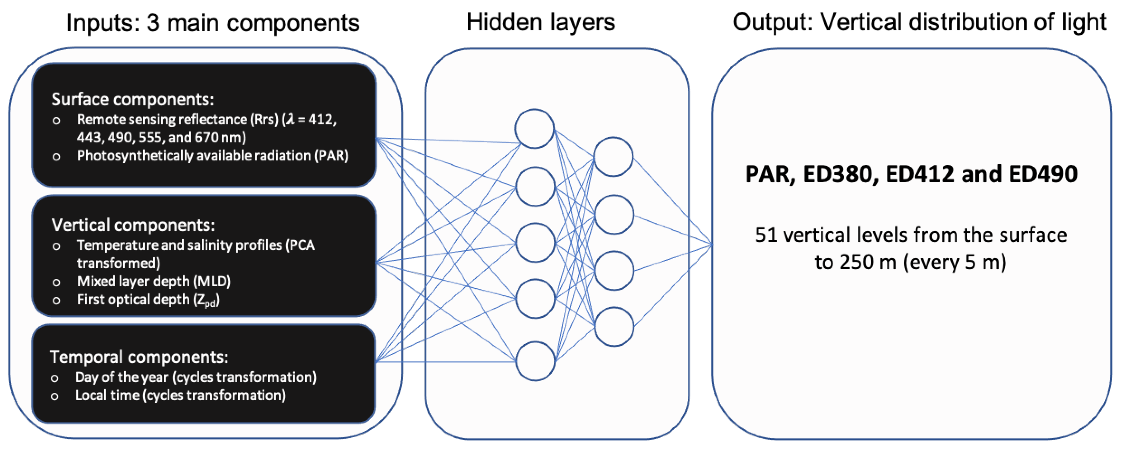
2.2.2. The SOCA-Light Models

For this study, we developed a SOCA-type model based on a neural network, and more specifically, a multilayer perceptron (MLP). The MLP is a robust modeling tool used for supervised learning, employing multiple inputs and a known output value to train the model [39,40,41]. As a feedforward neural network, information flows unidirectionally from the MLP’s input layer to its output layer, passing through one or more intermediate layers, also called hidden layers. Each layer is constructed from neurons, which are fundamental transfer functions that generate outputs when inputs are applied. Each connection between neurons has its own weight. The backpropagation algorithm then adjusts the weights of the neurons in each layer to minimize the loss function using a first-order gradient-based optimizer.
The SOCA-light models are largely derived from the generic SOCA methodology described in [26,27]. They consist of four models capable of predicting the vertical profiles of PAR, ED380, ED412, and ED490 at a given geolocation, using as inputs the data from matchups with satellite ocean color products and the vertical profiles of T and S. For SOCA-light, we have slightly modified the input variables used for other SOCA models (i.e., for Chla and b b p ) through the selection of key variables that depict the vertical propagation of light in the water column (i.e., first optical depth ( Z p d )). In this way, while other SOCA models (Chla and b b p ) have used sea-level anomaly (SLA) as input to infer mesoscale processes that may impact the vertical distribution of phytoplankton biomass, in SOCA-light models we have removed SLA from the key variables. The four SOCA-light neural networks were trained using a database of concurrent profiles of temperature, salinity, and light variables (ED380, ED412, ED490, and PAR) collected by BGC-Argo floats and collocated with satellite-derived products. A schematic representation of all the SOCA-light models is shown in Figure 4.
There are three main input components used for this model:
  • Surface components: These encompass satellite-based surface estimates of R r s at five different wavelengths (i.e., 412, 443, 490, 555, and 670 nm) and PAR.
  • Vertical components: These rely on the first principal component analysis of salinity and temperature profiles. The principal components were selected on the basis of cumulative explained variance values less than or equal to 0.998. For temperature, this criterion is satisfied by five principal components, and for salinity, by four principal components. The mixed layer depth (MLD) was derived from density calculated from pressure, temperature and salinity profiles with a density differential threshold criterion of 0.03 kg m 3 with reference to the density at 10 m [42]. The Z p d was derived from the satellite-derived k d ( 490 ) using Equation (2).
    Z p d = 1 k d ( 490 )
  • Temporal components: The temporal components are the day of the year (DOY) and the local time (LT) of the sampling profile. These components follow periodic evolution within certain time windows (0 to 365 days for DOY; 0 to 24 h for LT). The cyclic transformations (sine and cosine) of radian-transformed DOY and LT were used as temporal components (Equations (3) and (4)):
D O Y r a d = D O Y × π 182.625
L T r a d = L T × π 12
The SOCA-light model outputs are the four light variables (PAR, ED380, ED412, and ED490) at 51 vertical levels from the surface to 250 m depth at every 5 m interval. The use of an ensemble of MLPs proved effective in improving the robustness and reliability of predictions compared to the use of a single MLP [43]. For this reason, as a first step, several MLPs were created, each with a unique architecture incorporating the hyperbolic tangent (tanh) as the activation function and adaptive moment estimation (ADAM) [44] as the solver. The ADAM solver streamlines the conclusion of iterations upon reaching model convergence, speeding up the process. At the same time, we identify the optimal number of epochs to ensure effective learning and prevent overfitting.The key distinction among these models lies in the varying number of neurons distributed across each hidden layer, with the intention of capturing diverse patterns and representations inherent in the data. We chose two hidden layers from the considered options of one, two, and three hidden layers for these light models. Notably, models with two hidden layers consistently outperformed, with the number of neurons in the second hidden layer always being fewer than or equal to that in the first hidden layer. The models were trained by changing the neuron numbers between 5 and 150 with an increment of one (altogether 10,585 iterations). The second step was then to select, from all these iterations, an ensemble of the 10 best MLPs based on minimum statistical metrics obtained from training and validation datasets (root mean square error (RMSE) and the median absolute percent error (MAPE)). Through this selection, the ensemble model aimed to capture diverse representations while ensuring the sound performance and consistency of individual MLPs.

2.2.3. Statistical Analyses

The performance of the model was evaluated by comparison between the modeled variable values (Y-axis) and the actual values used as references (X-axis). Two statistical criteria were used: the RMSE as well as the MAPE that were computed as in the equations below (Equations (5) and (6)):
R M S E = i = 1 n ( O b s i P r e d i ) 2 n
M A P E ( % ) = m e d i a n O b s i P r e d i O b s i × 100
where n, O b s , and P r e d correspond to the number of points, the observed value, and the predicted value, respectively.

3. Results

3.1. Validation of SOCA-Light Models

A rigorous set of validation protocols was adopted to assess the accuracy of the four light models. In this way, the model results were validated against the validation database (Section 3.1.1), then against the four independent BGC-Argo floats from four distinct oceanic basins (Section 3.1.2), as well as against the independent SeaBASS database (Section 3.1.3). Finally, proxies derived from SOCA-light products were further used to evaluate the prediction capability of the model (Section 3.1.4).

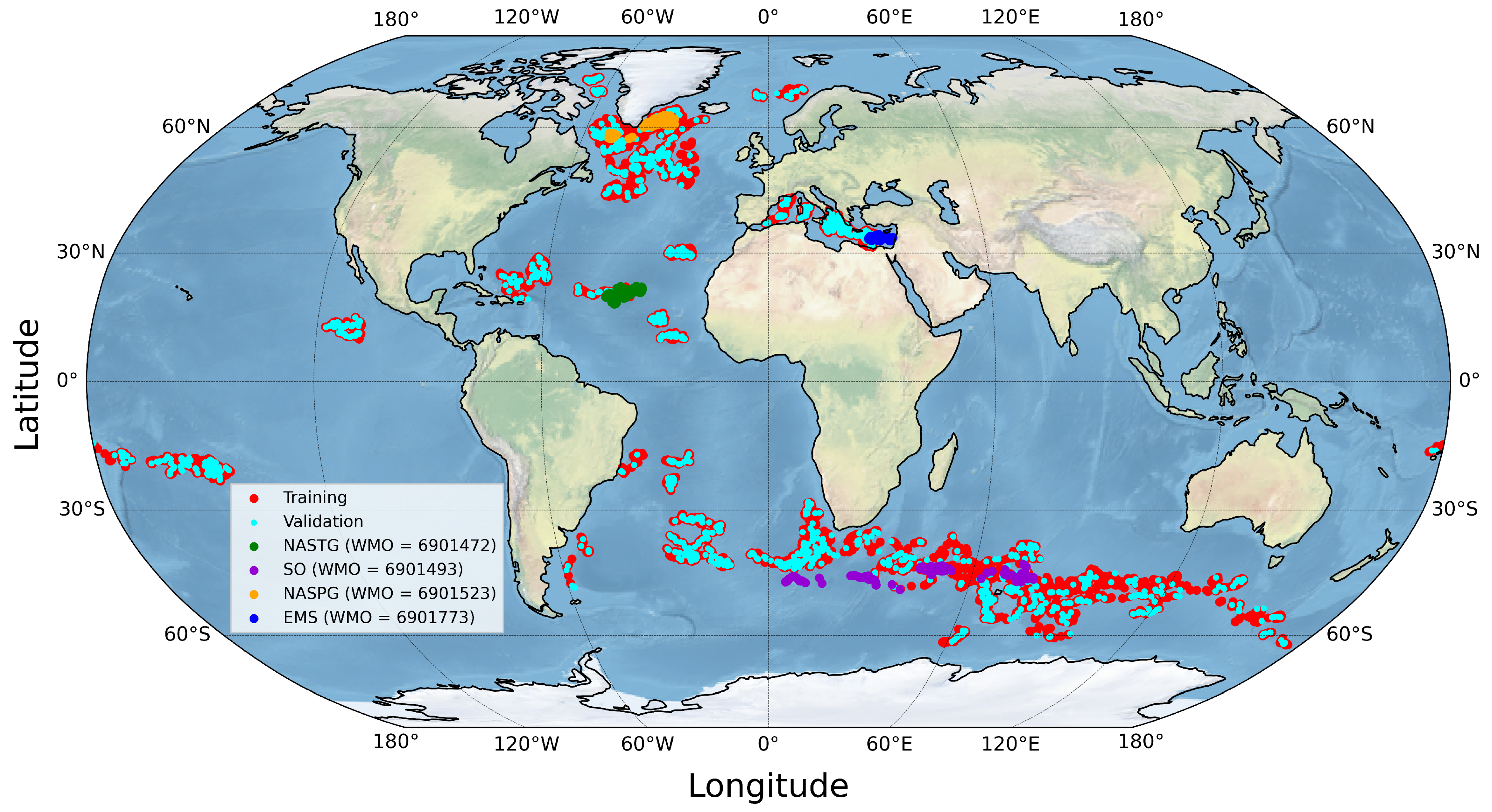
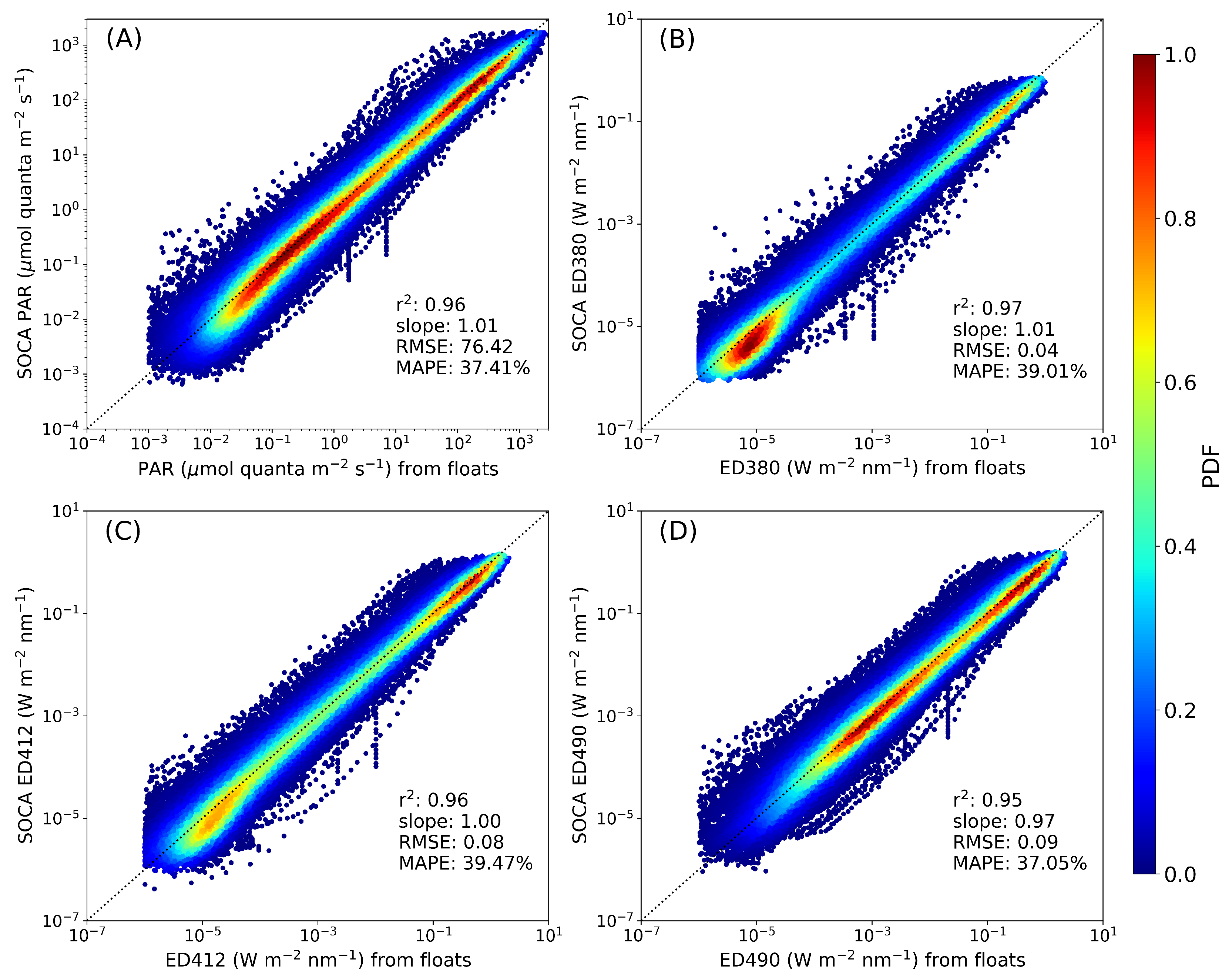
3.1.1. Validation of SOCA-Light Models Using 20% of the Global Database

The SOCA-light models were validated using 20% of the dataset randomly extracted from the BGC-Argo database, originating from a large diversity of oceanic regions. The comparison between modeled SOCA-light variables and BGC-Argo measurements (PAR, ED380, ED412, and ED490) is presented in Figure 5. Overall, there is a very good agreement between the predicted and the measured light variables. The density scatterplot reveals a close clustering of points along the identity line over more than five orders of magnitude. Statistical metrics extracted from linear regression between the modeled and observed PAR values reveal slope, r 2 , RMSE and MAPE values of 1.01, 0.96, 76.42 μmol quanta m 2 s 1 , and 37.41%, respectively (Figure 5A). The validation for the three ED models shows satisfactory performances. The modeled ED380 profiles exhibit RMSE and MAPE values of 0.04 W m 2 nm 1 , and 39.01%, respectively, when compared with their measured counterparts (Figure 5B). Similarly, the MAPE values for ED412 and ED490 were 39.47% and 37.05%, respectively (Figure 5C,D).

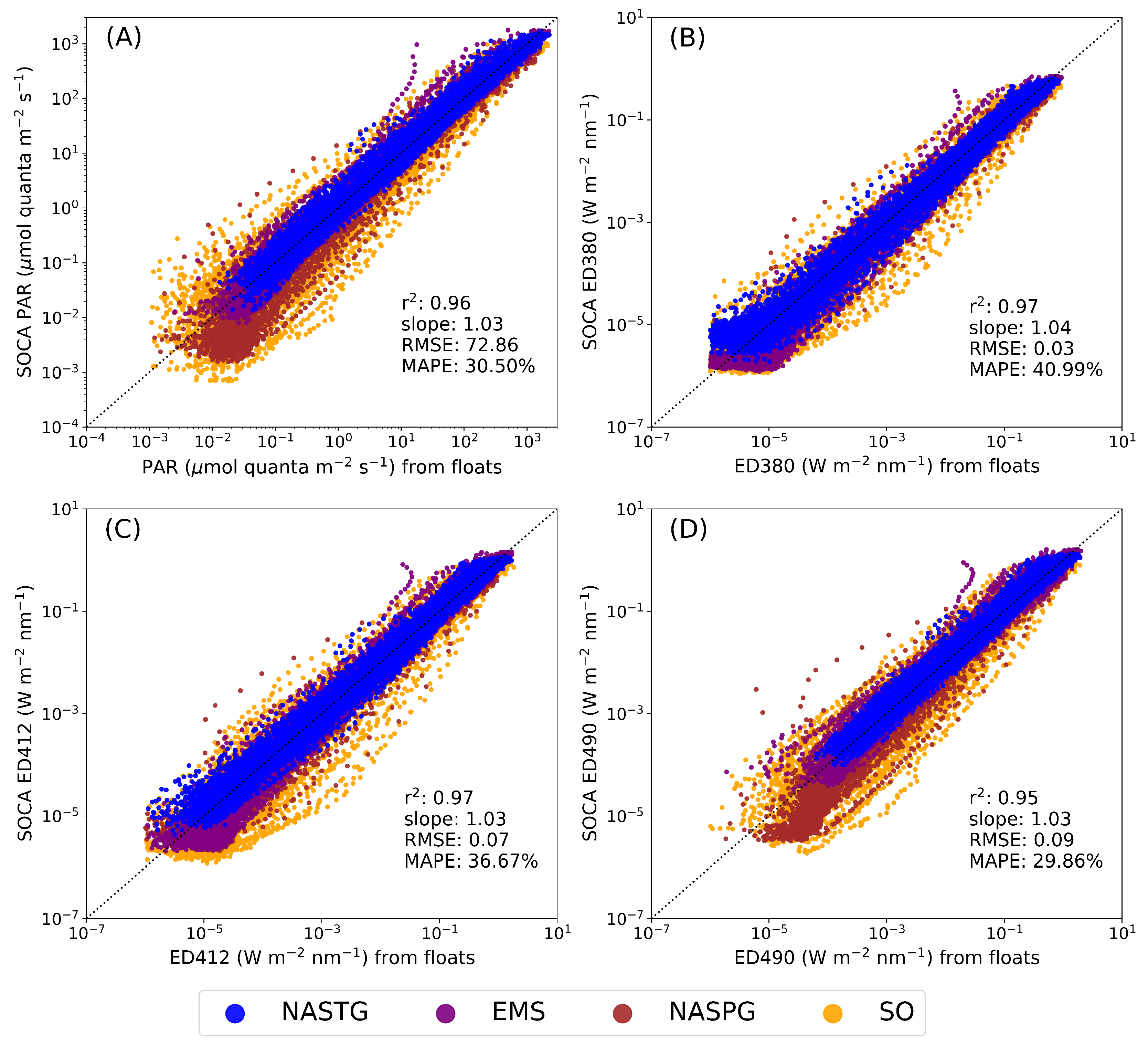
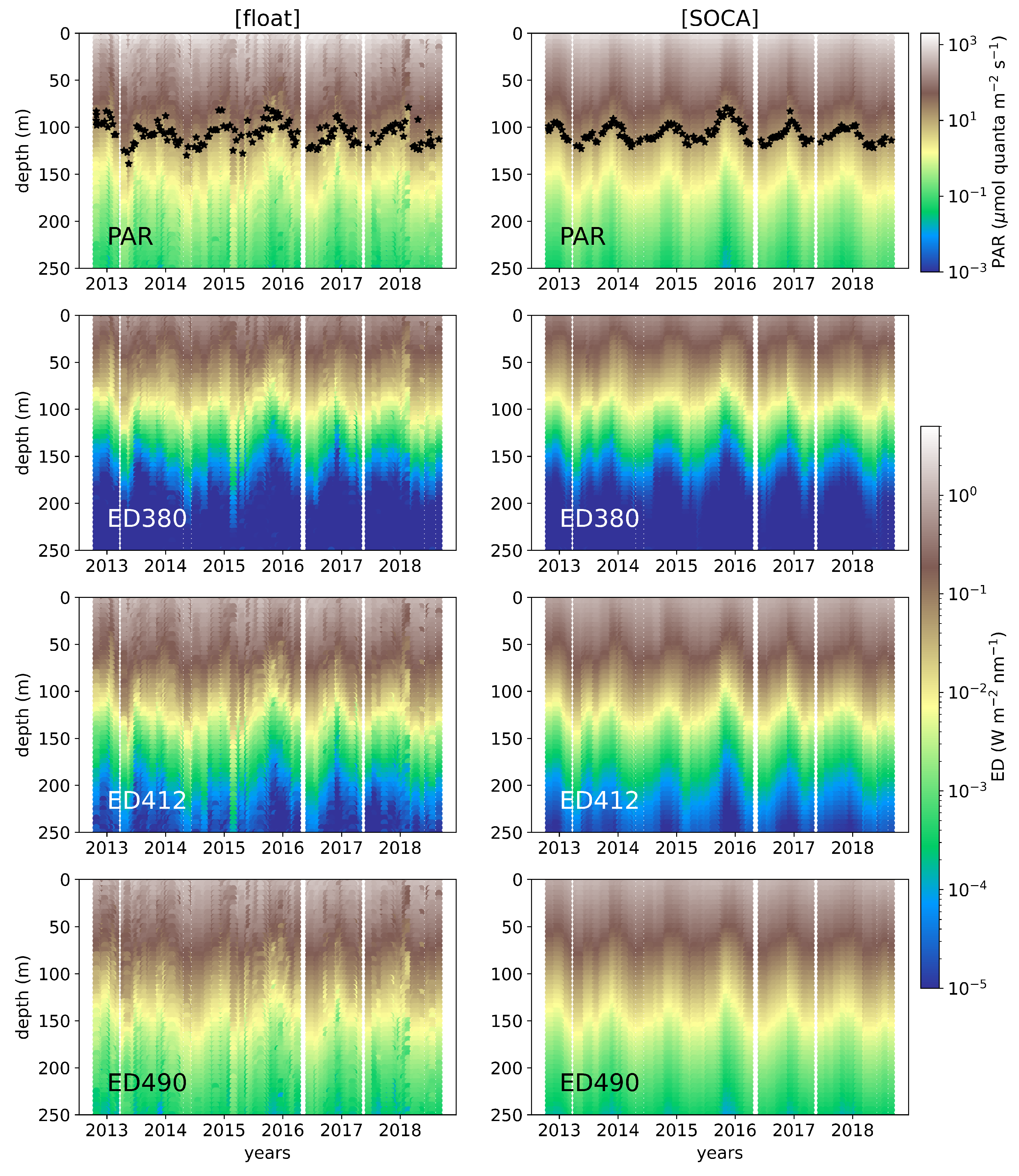
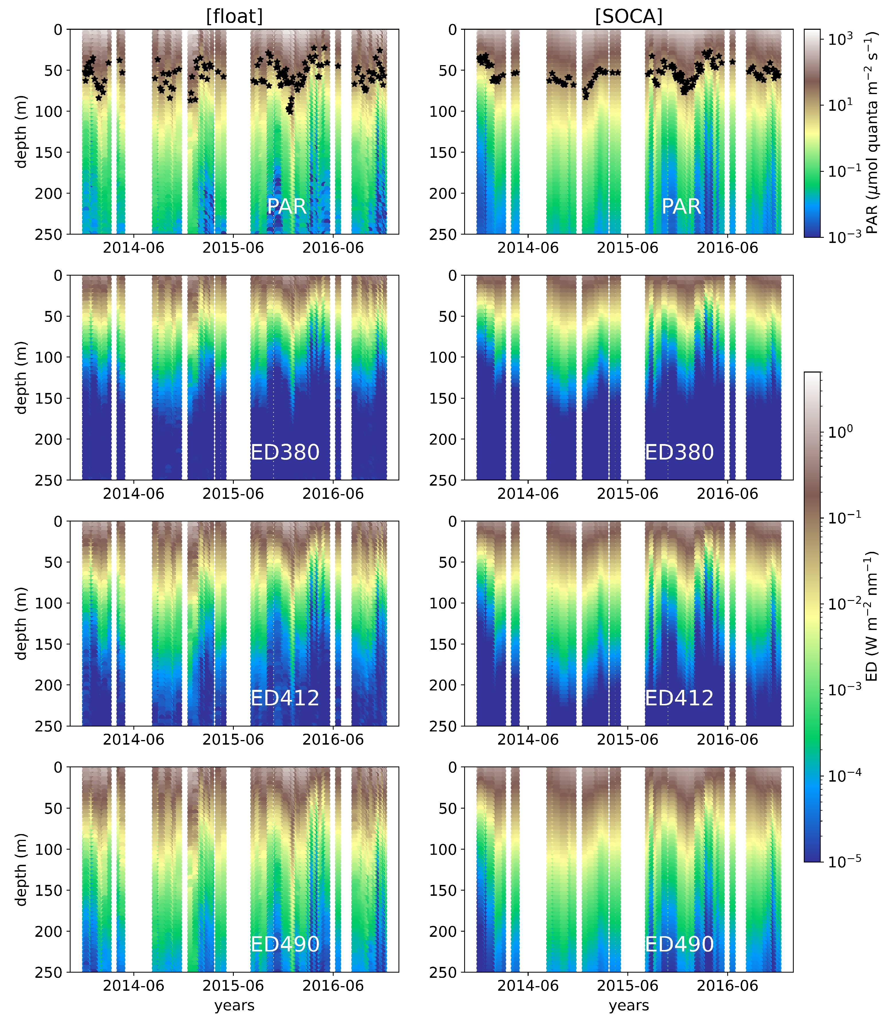
3.1.2. Validation of SOCA-Light Models Using Four Independent BGC-Argo Floats from Different Oceanic Regions

An independent validation was performed using four BGC-Argo floats from distinct oceanic regions, namely the North Atlantic Subtropical Gyre (NASTG), the Eastern Mediterranean Sea (EMS), the Southern Ocean (SO), and the North Atlantic Subpolar Gyre (NASPG). The profiles for each region originated from a single float with a unique WMO, none of which were included in the training and validation databases. The validation results for each oceanic region are presented in Figure 6.
The scatterplot of PAR derived by the model shows strong agreement with PAR measured by the BGC-Argo floats for all four regions (Figure 6A). Statistical error estimators computed between modeled and observed PAR profiles for all four regions together show slope, r 2 , RMSE, and MAPE values of 1.03, 0.96, 72.86 μmol quanta m 2 s 1 , and 30.50%, respectively. These statistical error estimators of PAR are comparable with the statistics obtained on 20% of the validation database (Figure 5A). For ED380 (Figure 6B), the slope, r 2 , RMSE, and MAPE values are 1.04, 0.97, 0.034 W m 2 nm 1 , and 40.99%, respectively. For ED412 (Figure 6C), the same statistical metrics yield values of 1.03, 0.97, 0.070 W m 2 nm 1 , and 36.67%, respectively. Finally, for ED490 (Figure 6D), the metrics take values of 1.03, 0.95, 0.087 W m 2 nm 1 , and 29.86%, respectively.

North Atlantic Subtropical Gyre

The NASTG is an oligotrophic environment characterized by low surface nutrients, low Chla, and the presence of a permanent deep chlorophyll maximum (DCM), generally found below 100 m [45,46]. The multi-year time series (more than 6 years of measurement) of the vertical distribution of light variables (PAR, ED380, ED412, and ED490) measured by the NASTG BGC-Argo float (WMO = 6901472) and modeled by SOCA-light are presented in Figure 7 for a direct comparison. Overall, the SOCA-light models clearly reproduce, in a smoother way, the seasonal and vertical trends revealed by the float measurements. The SOCA-light models capture even subtle changes in the general trends of light variables, as evidenced by the less pronounced light penetration observed and reproduced by the model at the end of 2015. As well as reproducing the trends satisfactorily, the magnitude of the signals is retrieved well by the models for the four variables. The statistical metrics between the modeled and the observed PAR profiles show (Figure S4) slope, r 2 , RMSE, and MAPE values of 0.99, 0.98, 73.09 μmol quanta m 2 s 1 , and 21.50%, respectively. For ED380, these metrics are, respectively, 0.96, 0.98, 0.04 W m 2 nm 1 , and 28.72%. For ED412, they are 0.95, 0.98, 0.08 W m 2 nm 1 , and 26.66%. Finally, for ED490, they are 0.98, 0.98, 0.09 W m 2 nm 1 , and 21.53%.

Eastern Mediterranean Sea

The EMS is also a permanent oligotrophic system at temperate latitudes. The float selected (WMO = 6901773) measured all four light variables (PAR, ED380, ED412, and ED490) for nearly four years (Figure S5). Again, the multi-year vertical sections of these variables from this region show very good agreement between the measured and modeled values. The modeled variables exhibited seasonal fluctuations in their magnitude across different years, similar to those observed. The surface incoming solar radiation shows larger seasonal variability than the variability observed in the subtropical oligotrophic regime (NASTG, Figure 7), yet it is well captured by the model. As for the NASTG, the models reproduce light variables with much less noise compared to their corresponding BGC-Argo measurements. The statistical metrics between the modeled and the measured variables from the EMS for all four light variables are highly comparable with the global 20% validation metrics (Figure S6). The statistical metrics between the modeled and the observed PAR profiles display slope, r 2 , RMSE, and MAPE values of 1.02, 0.98, 63.20 μmol quanta m 2 s 1 and 21.42%, respectively. For ED380, these metrics were, respectively, 1.08, 0.98, 0.03 W m 2 nm 1 , and 39.89%. For ED412, they were 1.06, 0.98, 0.06 W m 2 nm 1 , and 29.04%. Lastly, for ED490, they were 1.01, 0.98, 0.08 W m 2 nm 1 , and 22.78%. All the derived error estimators show comparable values (some even better, such as the RMSE and MAPE) with those obtained for the 20% global validation database. These results depict the robustness of the SOCA-light models for deriving light variables over several years of observation.

Southern Ocean

Over four years, the BGC-Argo float (WMO = 6901493) traveling eastwards (from 5 ° E to 83 ° E) and between 40 ° S and 50 ° S in the SO underwent the typical bio-physical conditions prevailing in the area. Overall, it captured four phytoplankton blooms and was regularly trapped or influenced by mesoscale features or fronts. The multi-year time series of the vertical distribution of light variables (PAR, ED380, ED412, and ED490) measured by this float and the SOCA-light modeled light variables are presented and compared in Figure 8. The gaps in the time series during the southern-hemisphere winter months are due to the unavailability of ocean color matchups resulting from cloud coverage during this period. In general, as for the NASTG and EMS, the SOCA-light models reproduce the seasonal and vertical trends of the float measurements in a smoother way. In addition to reproducing the seasonal trends, the magnitude of the retrieved light variables is in order with the measurements for the four light variables. The statistical metrics between the modeled and measured PAR profiles (Figure S7) show slope, r 2 , RMSE, and MAPE values of 0.99, 0.91, 88.63 (μmol quanta m 2 s 1 ), and 54.37%, respectively. For ED380, these metrics were 1.03, 0.95, 0.04 (W m 2 nm 1 ), and 51.52%. For ED412, they were 1.03, 0.93, 0.08 (W m 2 nm 1 ), and 54.33%. Finally, for ED490, the metrics were 0.99, 0.91, 0.10 (W m 2 nm 1 ), and 51.47%. The statistical estimators from the SO, namely the RMSE and MAPE, are slightly larger than the global 20% validation metrics. These uncertainties could possibly originate from the highly dynamic nature of the area associated with the ocean color matchups of the closest pixel of the temporal (±5 days) and spatial (5 × 5 pixels) matchups. They may also be attributed to the higher level of this dataset’s independence, thus providing a more rigorous test of the model’s generalization capabilities. Indeed, a higher level of errors can be expected in a highly variable environment such as the SO. Nevertheless, the fact that errors from this dataset are only marginally greater than those from the 20% validation dataset suggests the model’s robustness without signs of overfitting.

North Atlantic Subpolar Gyre

The data acquired by the float (WMO = 6901523) over its two years of exploration are representative of the diversity of the North Atlantic Subpolar Gyre conditions. In particular, it encountered intense convection periods (>1000 m) as well as intense spring phytoplankton blooms. Due to a lack of ocean color matchups, the NASPG region experienced similar problems as the SO region in obtaining SOCA-light variables during the winter. The two-year time series of the vertical distribution of light variables (PAR, ED380, ED412, and ED490) measured by this float and modeled by SOCA-light are presented and compared in Figure S8. Essentially, the SOCA-light models reproduce the seasonal trends in float measurements in a smoother way. The statistical metrics between the modeled and the observed PAR profiles manifest slope, r 2 , RMSE, and MAPE values of 1.08, 0.93, 64.83 μmol quanta m 2 s 1 , and 58.79%, respectively (Figure S9). For ED380, these metrics were subsequently 1.02, 0.96, 0.02 W m 2 nm 1 , and 50.82%. For ED412, they were 1.02, 0.95, 0.04 W m 2 nm 1 , and 51.75%. Finally, for ED490, these metrics were 1.09, 0.92, 0.06 W m 2 nm 1 , and 57.63%. Similarly to the SO float, the statistical estimators, mainly the RMSE and MAPE, from the NASPG float are slightly larger than the global 20% validation metrics. This could mainly be due to the uncertainties associated with the retrieval of ocean color matchups from the closest pixel of the temporal (±5 days) and spatial (5 × 5 pixels) matchups in such a highly dynamic high-latitude environment, which seems less the case for low and temperate latitudes (see Figure 7 and Figure S5 and the associated metrics in Figures S4 and S6).

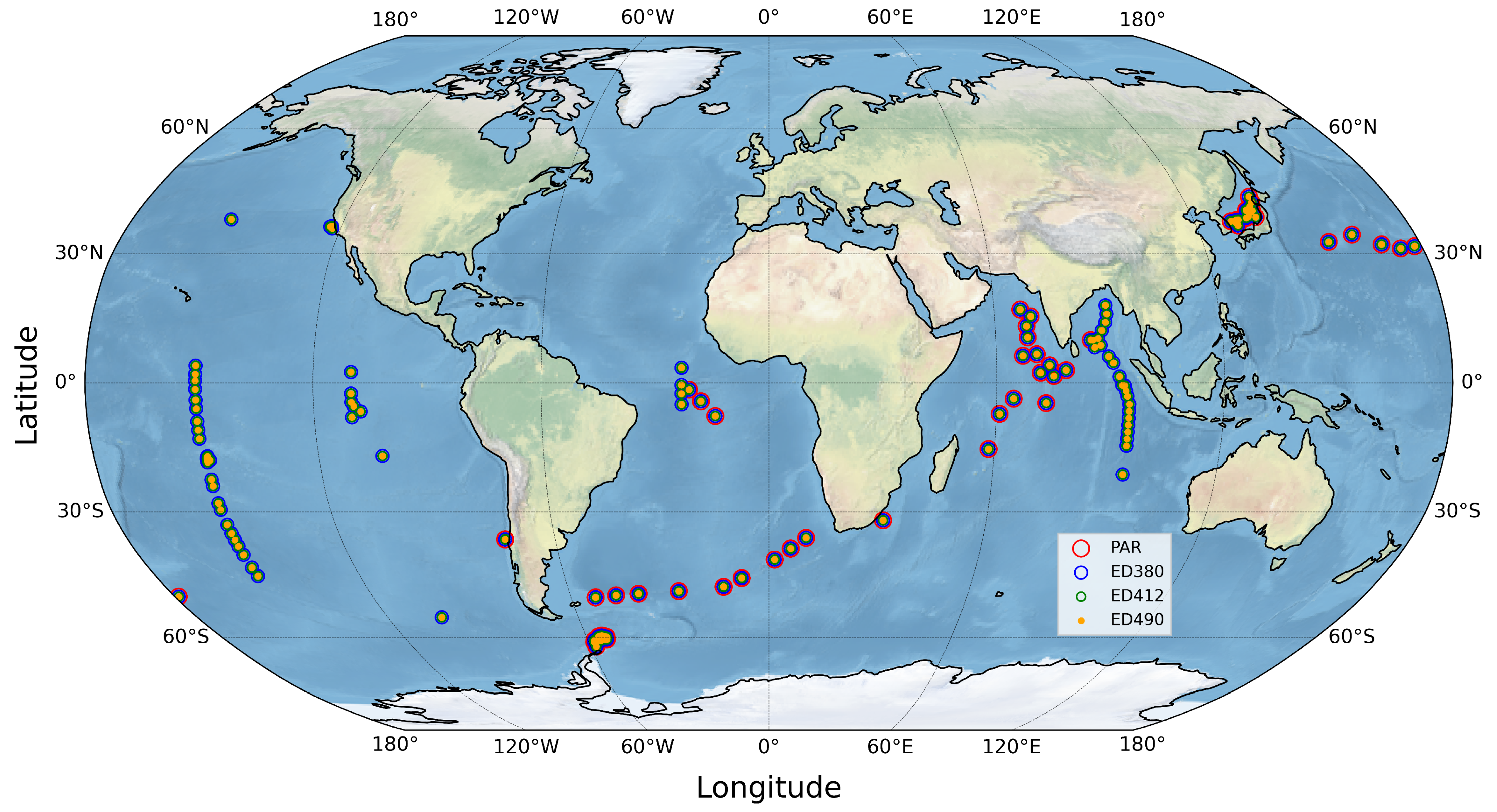
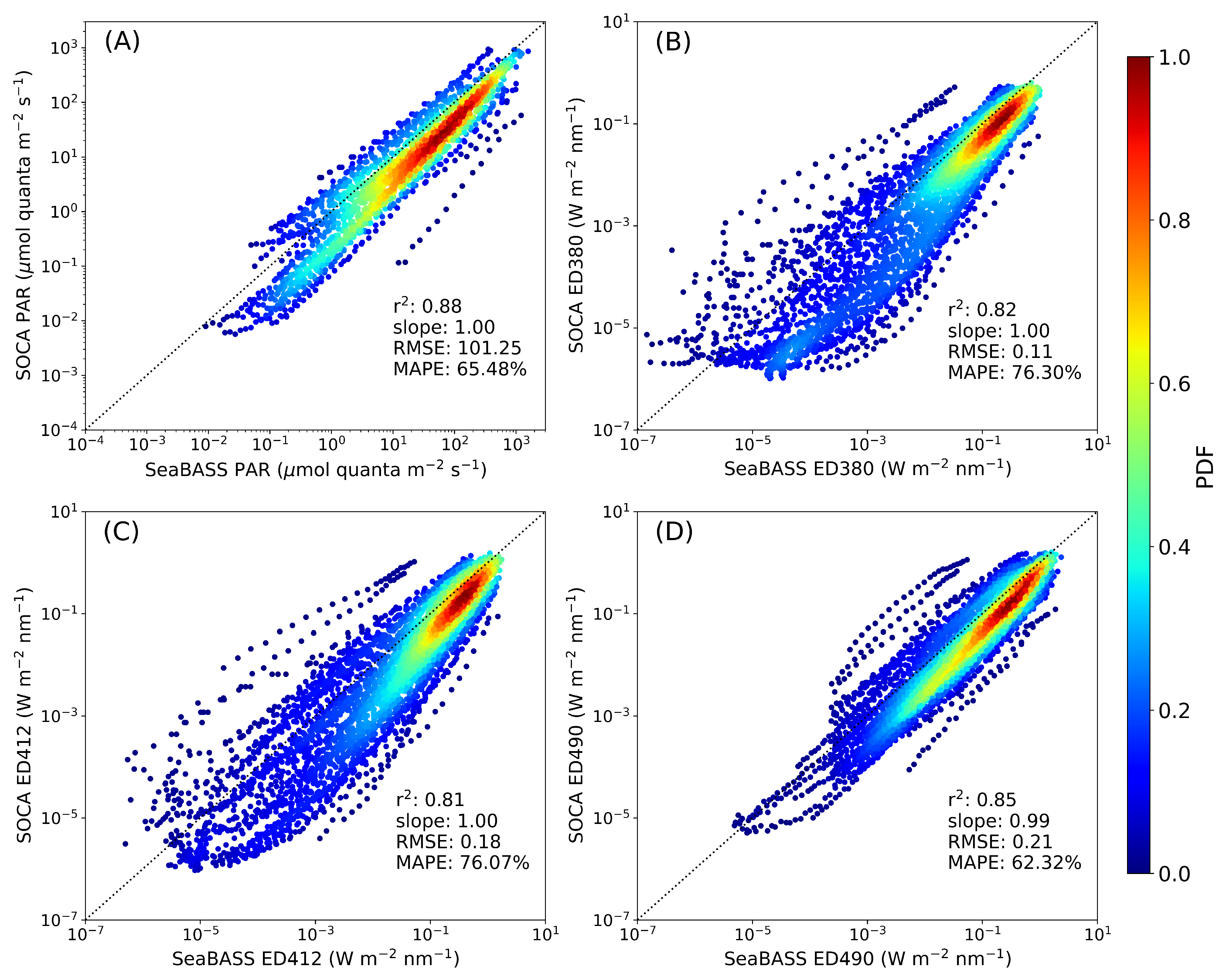
3.1.3. Validation of SOCA Light Models with the Independent Global SeaBASS Database

As well as validating SOCA-light models against a 20% subset of the BGC-Argo dataset or against the data of selected BGC-Argo floats not included in either the initial training or the 20% validation procedures, validation against datasets not acquired by BGC-Argo offered an informative complementary exercise. For this purpose, we used the global SeaBASS light database whose measurements originate from various cruises and field campaigns. It should be noted that, contrary to the BGC-Argo light measurements performed under any sky conditions, measurements from ships, which are more operator-dependent, are essentially conducted under a clear sky.
The input matchups were taken from the weekly binned files of ARMOR3D and GlobColour data that corresponded to each SeaBASS in situ station. The physical variables (temperature, salinity, and MLD) were extracted from the macro-pixel (0.25 ° × 0.25 ° ) nearest the in situ station and ocean color matchups from the mean of the 3 × 3 micro-pixels (4 km × 4 km) box centered at each in situ station. It should be noted that only a restricted number of stations from the original SeaBASS database were used for this validation exercise, as more than 90% of the stations (including coastal stations with bathymetric depths less than 1500 m) lacked a corresponding satellite ocean color matchup, mainly due to the contamination of signals, probably by clouds or sea ice.
The scatterplots of the light variables derived by the SOCA-light models compared with those measured in situ within the SeaBASS database are presented in Figure 9. The same metrics are reported as those in the other validation exercises based on float data (Section 3.1.1 and Section 3.1.2). Figure 9 shows that the retrieval by SOCA-light systematically underestimates the SeaBASS measurements for each light variable. This bias is the same over the whole water column as the slopes between the modeled light and corresponding measurements are close to one (Figure 9). The fact that the SeaBASS database is essentially populated by data obtained under clear-sky conditions at a given time could explain this bias. By way of contrast, the weekly matchups of GlobColour products used as input for the SOCA-light models likely do not correspond to clear-sky conditions over such an extended temporal window.
The scatterplot of PAR produced by the model exhibits notable consistency with PAR measured in situ by SeaBASS data (Figure 9A). Statistical error metrics were extracted from linear regression between the modeled and observed PAR profiles, showing slope, r 2 , RMSE, and MAPE values of 1.00, 0.88, 101.25 μmol quanta m 2 s 1 , and 65.48%, respectively. For ED380, these metrics were 1.00, 0.82, 0.11 (W m 2 nm 1 ), and 76.30% (Figure 9B). For ED412, they were 1.00, 0.81, 0.18 W m 2 nm 1 , and 76.07% (Figure 9C). Finally, for ED490, they were 0.99, 0.85, 0.21 W m 2 nm 1 , and 62.32% (Figure 9D). These four light models (PAR, ED380, ED412, and ED490) were validated independently, and the extracted error metrics are quite satisfactory, even if these statistical estimators are slightly larger compared with the error metrics of both the global 20% validation database and four independent BGC-Argo floats. These larger error estimators could be because of the uncertainty associated with the physical and ocean color data considered as inputs (as well as the nature of the data in SeaBASS, essentially acquired under clear-sky conditions).

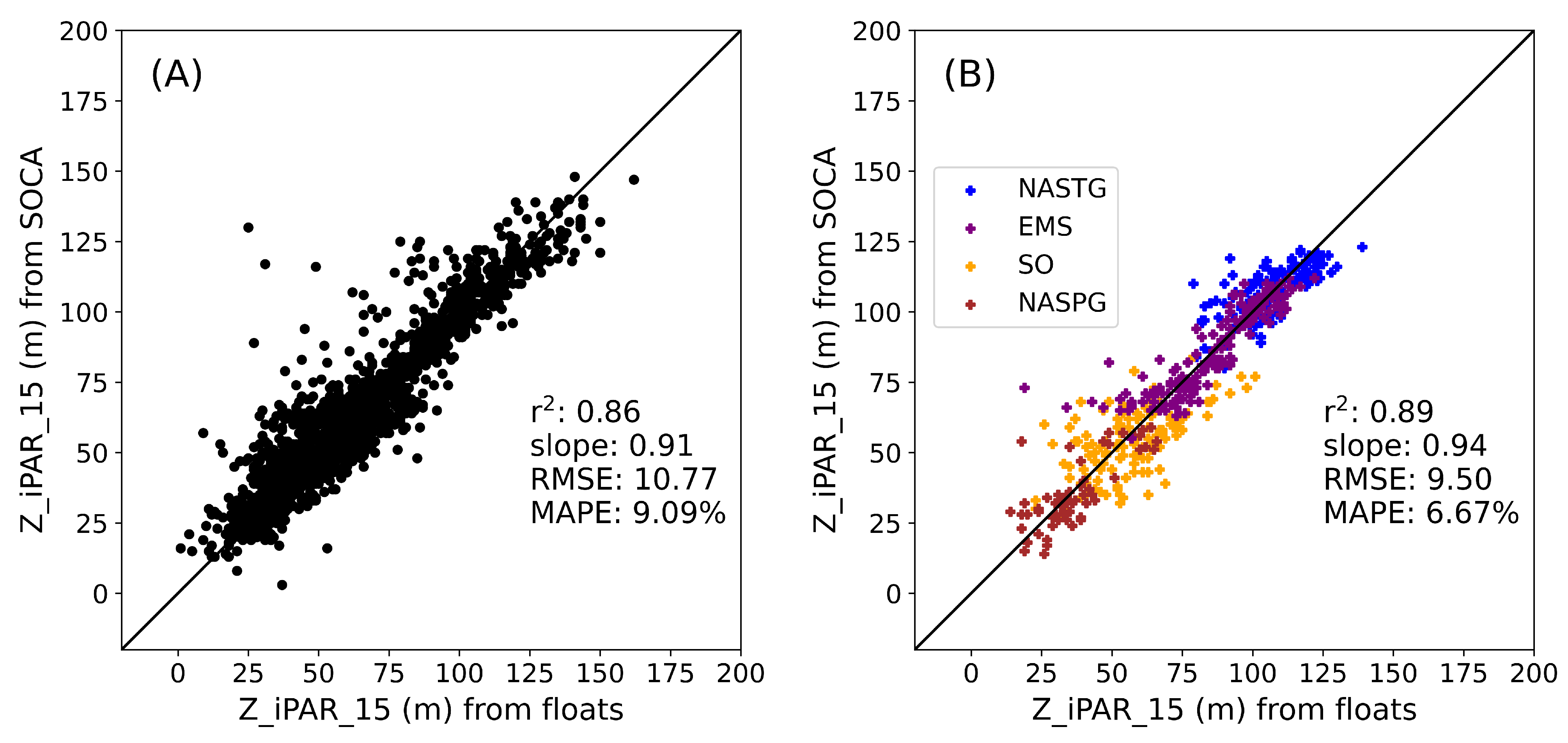
3.1.4. Additional Validation with iPAR_15

An alternative to validating the SOCA-light model results against light data from various databases (previous sections), that also allows gauging the model’s prediction capabilities, is to quantify and assess the quality of model-derived products that are essential for certain applications. This is the case for the depth of iPAR_15 (Z_iPAR_15) [47], a variable that corresponds to the depth at which the instantaneous PAR, iPAR, equals 15 μmol quanta m 2 s 1 . This quantity is required for the correction of non-photochemical quenching (NPQ) that affects the chlorophyll-a fluorescence profiles. NPQ is a photo-physiological mechanism whereby the signal of chlorophyll-a fluorescence is depressed under high irradiances (maximal at noon). The method proposed by [47] and further improved by [48] uses Z_iPAR_15 as a depth threshold under which no NPQ is expected. In a way, Z_iPAR_15 can be considered as a proxy for water clarity with high values corresponding to the clearest waters, where the NPQ effect can be observed at the deepest depths. The present study extracted Z_iPAR_15 from PAR measured by the BGC-Argo floats and PAR derived using the SOCA-light PAR model for the validation database of 20% of the global database and for the four independent floats (Figure 10). Overall, the results are satisfactory with respect to the retrieval of Z_iPAR_15 by the SOCA-light PAR model. Furthermore, the range of values of Z_iPAR_15 for the four floats (Figure 10B) is equivalent to that for the 20% validation database (Figure 10A). This demonstrates that the four floats cover the entire range of trophic status currently detected by the BGC-Argo database throughout the global ocean.
To illustrate a potential application of the SOCA-light models, we extracted global 3D multi-year monthly averaged climatologies of light variables at local noon at a 5 m resolution from the surface to 250 m depth. The inputs used to generate the climatologies were multi-year monthly averaged GlobColour data and ARMOR3D physical data. The satellite data were averaged (0.25 ° × 0.25 ° ) at the same spatial resolution as the physical ARMOR3D data. As an example, the extracted Z_iPAR_15 from these seasonal climatology fields is presented in Figure 11, and shows well-characterized latitudinal and seasonal variations.

4. Discussion and Conclusions

Knowledge about the irradiance vertical distribution is essential for improved understanding and quantification of many oceanic processes in the upper water column. Over time, a variety of bio-optical models has been developed to better predict light fields, particularly at the ocean surface. These models have drawn from various complex relationships, spanning from purely empirical to fully analytical algorithms. They have served as fundamental building blocks for various biogeochemical applications, including the retrieval of IOPs [49,50], biogeochemical quantities such as Chla [51,52,53], and POC [54], as well as the quantification of the oceanic heating rate [3,4] and the modeling of oceanic primary production [1,2]. These models serve as the foundation for bio-optical oceanography and satellite ocean color science.
The development of bio-optical models has, however, been constrained by the limited availability of in situ data, either for model construction (for empirical models) or model validation (in the case of analytical models). Substantial gaps in the acquisition of bio-optical data have resulted in limited coverage and sparse datasets, especially in remote open ocean areas. Additionally, the databases containing these measurements often exhibit heterogeneity in terms of acquisition modes, involving different platforms and sensors. These variations lead to consistency and interoperability issues, increasing the uncertainties of models relying on these data.
More recently, the prospect of developing more accurate bio-optical models for irradiance vertical distribution has emerged for two main reasons. The first one relates to the massive availability of the various oceanic properties, including optically significant substances and light variables. This availability is largely due to the extensive data-collection capacity of BGC-Argo, which has contributed to a rich and dense database of ED and PAR profiles. Importantly, in addition to being publicly and openly accessible, this database offers the advantage of being homogeneous and interoperable thanks to the development of dedicated methods to ensure its qualification [29,55,56]. Moreover, this database has proven instrumental in validating bio-optical models [57,58] and models based on Chla for estimating PAR [22]. The second reason is due to the increasing adoption of machine learning techniques that take advantage of data availability, which results in a strong improvement in the predictive capability of these purely empirical approaches. Pioneering work by [26] showed that global 3D reconstruction of the b b p could be performed thanks to the development of the first SOCA model. More recently, subsets of irradiance data (ED380, ED412, and ED490) acquired by BGC-Argo floats have been used to predict PAR either through statistical approaches [59] or the use of neural networks [60].
The present study represents, to our best knowledge, the first attempt to develop a predictive model for the vertical profiles of light, encompassing both PAR and irradiance at three different wavelengths, thanks to the application of machine learning using the extensive BGC-Argo light database. This model rests on the initial SOCA methodology, which has been carefully refined to accommodate the specificity of light-related variables. While the model exhibits significant accuracy and potential, it does have some limitations that should be acknowledged. Certainly, the prediction of light profiles becomes challenging in the absence of R r s data (e.g., due to cloud coverage), a situation particularly critical in high-latitude environments during the winter. Moreover, the majority of SOCA-light training involved local noon data (97% of profiles gathered between 10 and 13 h local time), suggesting a potential decrease in accuracy for predictions at other times of the day. Nevertheless, as more data from BGC-Argo become available at various times, this limitation could be easily addressed in the near future. In the meantime, it is recommended to preferentially use SOCA-light around noon local time.
The predictive power of SOCA-light appears to be robust (Figure 5, Figure 6, Figure 9 and Figure 10). Until now, efforts to characterize vertical light profiles in oceanic waters have relied on various approaches, involving numerical models [17,18,19,20,21] and a combination of analytical, semi-analytical, and empirical relationships [11,20,22,33]. However, these models heavily rely on specific parameters, including AOPs, IOPs, and Chla resolved over the vertical dimension. The incorporation of these precise vertically resolved inputs presents challenges when attempting to compare such models with SOCA-light ones. The lack of these crucial input data poses a well-acknowledged challenge in the field of oceanography, especially within the marine optics and ocean color remote sensing communities. Consequently, this data gap potentially translates into more uncertainty over depths. The machine learning approaches proposed here potentially circumvent this weakness. Furthermore, assuming the model inputs are at the right resolution, SOCA-light can easily extract 3D global ocean light maps at any temporal resolution (daily, weekly, and monthly).
Due to their solidity and versatility, SOCA-light models offer great potential for supporting many applications for which light profiles are key variables but are unfortunately not measured. For instance, several applications for improving the BGC-Argo database can already be envisioned. At present, light profiles are not acquired from all BGC-Argo floats. Indeed, less than 45% of the ≈118,000 chlorophyll-a fluorescence profiles so far acquired have concurrent light measurements. Yet, light profiles are required for a more accurate estimation of Chla from chlorophyll-a fluorescence measured from floats. First, the correction of NPQ fluorescence is more accurate with the use of instantaneous PAR profiles [47,48] compared to former methods which do not rely on light [61]. Secondly, as the relation between Chla and chlorophyll-a fluorescence varies regionally and seasonally, methods have been proposed that rely on concurrent profiles of ED490 and chlorophyll-a fluorescence to estimate the slope correction to apply to the fluorescence profile in order to retrieve more accurate Chla [6]. The estimation of this slope correction relies on a bio-optical relationship linking k d ( 490 ) (derived from the ED490 profile) to Chla [11]. Having the whole BGC-Argo fleet delivering light profiles (either measured or modeled) would guarantee an overall more consistent and interoperable Chla dataset. Similar methods would allow the derivation of profiles of CDOM absorption at 412 nm from profiles of CDOM fluorescence, calibrated chlorophyll-a fluorescence (slope correction applied), and irradiance (ED412) [8]. Therefore, the potential of SOCA-light already appears enormous when simply considering its possible applications in relation to the BGC-Argo database alone.
Recently, floats have begun to acquire hyperspectral radiometric measurements [62,63]. New perspectives that consequently open up include refinements in the characterization of optically active substances, such as CDOM or phytoplankton community structure at large scale [63]. The SOCA-light method presented here has the potential to accommodate any increase in the spectral domain and resolution once sufficient data have been acquired to support training. The availability of such modeled data could represent a new step towards a better understanding of various components of biogeochemical cycles at a global scale.

Supplementary Materials

The following supporting information can be downloaded at: https://www.mdpi.com/article/10.3390/rs15245663/s1, Figure S1: Geographical distribution of BGC-Argo profiles used for the development and validation of the SOCA-light model for ED380, Figure S2: Geographical distribution of BGC-Argo profiles used for the development and validation of the SOCA-light model for ED412, Figure S3: Geographical distribution of BGC-Argo profiles used for the development and validation of the SOCA-light model for ED490, Figure S4: Scatter-plots between light variables (PAR, ED380, ED412, and ED490) modeled by SOCA light models versus their corresponding BGC-Argo measurements from NASTG. PAR (A); ED380 (B); ED412 (C); ED490 (D), Figure S5: Time series of the vertical distribution of the four light variables in the Easter Mediterranean Sea (EMS) measured by BGC-Argo float WMO 6901773 (left column) and modeled by SOCA-light (right column). The variables in each subplot are indicated by text in the corresponding subplots. The black stars indicate the depth at which instantaneous PAR value = 15 µmol quanta m 2 s 1 , Figure S6: Scatter-plots between light variables (PAR, ED380, ED412, and ED490) modeled by SOCA light models versus their corresponding BGC-Argo measurements from EMS. PAR (A); ED380 (B); ED412 (C); ED490 (D), Figure S7: Scatter-plots between light variables (PAR, ED380, ED412, and ED490) modeled by SOCA light models versus their corresponding BGC-Argo measurements from SO. PAR (A); ED380 (B); ED412 (C); ED490 (D), Figure S8: Time series of the vertical distribution of the four light variables in the North Atlantic Subpolar Gyre (NASPG) measured by BGC-Argo float WMO 6901523 (left column) and modeled by SOCA-light (right column). The variables in each subplot are specified by text in the corresponding subplots. The black stars indicate the depth at which instantaneous PAR value = 15 μmol quanta m 2 s 1 , Figure S9: Scatter-plots between light variables (PAR, ED380, ED412, and ED490) modeled by SOCA light models versus their corresponding BGC-Argo measurements from NASPG. PAR (A); ED380 (B); ED412 (C); ED490 (D). All of the models and functions (Jupyter Notebook) are open source and can be accessed via our GitHub page: https://github.com/renoshpr/SOCA-LIGHT-MODELS, (accessed on 10 November 2023).

Author Contributions

All the authors (P.R.R., J.Z., R.S. and H.C.) contributed to conceptualizing the methodology; P.R.R. implemented the methodology, the validation and formal analysis of results; P.R.R. wrote the initial draft; P.R.R., R.S. and H.C. revised and finalized the manuscript. All authors have read and agreed to the published version of the manuscript.

Funding

This study is a contribution to the following projects: REFINE (European Research Council, Grant agreement 834177), BGC-Argo-France (CNES-TOSCA), and the Copernicus Marine Environment Monitoring System (CMEMS) Ocean Multi-Observation TAC.

Data Availability Statement

The BGC-Argo data used in this study are publicly available at ftp://ftp.ifremer.fr/ifremer/argo, accessed on 17 February 2023, and supplied by the international Argo program. The ocean color (except surface PAR) and ARMOR3D data are publicly available at https://data.marine.copernicus.eu/products, (accessed on 17 February 2023) delivered by the Copernicus Marine Service. The ocean surface PAR data can be downloaded from the GlobColour portal from the following link https://hermes.acri.fr/?class=archive, (accessed on 17 February 2023) provided by ACRI-ST. The SeaBASS data are publicly available from the following link https://seabass.gsfc.nasa.gov/, (accessed on 17 February 2023) provided by the National Aeronautics and Space Administration (NASA).

Acknowledgments

These light profiles and physical variables (P, T, and S) were collected in the framework of the BGC-Argo program and made freely available by the International Argo program. The authors are also thankful to CMEMS for ocean color and physical data. The authors are grateful to NASA for the SeaBASS data.

Conflicts of Interest

The authors declare no conflict of interest relevant to this study.

Abbreviations

The following abbreviations are used in this manuscript:
ADAMAdaptive moment estimation
ANNArtificial neural network
AOPApparent optical property
ARMOR3DA 3D multi-observations T, S, U, V product of the ocean
b b p Particulate backscattering coefficient
BGC-ArgoBioGeoChemical Argo
CDOMColored dissolved organic matter
ChlaChlorophyll-a concentration
CMEMSCopernicus Marine Environment Monitoring System
DCMDeep chlorophyll maxima
DOCDissolved organic carbon
DOYDay of the year
EDDownwelling irradiance
EMSEastern Mediterranean Sea
GOOSGlobal Ocean Observing System
IOPInherent optical property
k d Diffuse attenuation coefficient
LTLocal time
LUUpwelling radiance
MAPEMedian absolute percent error
MLDMixed layer depth
MLPMultilayer perceptron
NASPGNorth Atlantic Subpolar Gyre
NASTGNorth Atlantic Subtropical Gyre
NNNeural network
PARPhotosynthetically available radiation
PDFProbability density function
POCParticulate organic carbon
RMSERoot mean squared error
R r s Remote sensing reflectance
SeaBASS    SeaWiFS Bio-Optical Archive and Storage System
SLASea-level anomaly
SOSouthern Ocean
SOCASatellite Ocean Color merged with Argo data
tanhHyperbolic tangent
WMOWorld Meteorological Organization
Z_iPAR_15The depth at which instantaneous PAR value = 15 μmol quanta m 2 s 1

References

  1. Antoine, D.; Morel, A. Oceanic primary production: 1. Adaptation of a spectral light-photosynthesis model in view of application to satellite chlorophyll observations. Glob. Biogeochem. Cycles 1996, 10, 43–55. [Google Scholar] [CrossRef]
  2. Westberry, T.; Behrenfeld, M.J.; Siegel, D.A.; Boss, E. Carbon-based primary productivity modeling with vertically resolved photoacclimation. Glob. Biogeochem. Cycles 2008, 22, GB003078. [Google Scholar] [CrossRef]
  3. Ohlmann, J.C.; Siegel, D.A.; Mobley, C.D. Ocean Radiant Heating. Part I: Optical Influences. J. Phys. Oceanogr. 2000, 30, 1833–1848. [Google Scholar] [CrossRef]
  4. Ohlmann, J.C.; Siegel, D.A. Ocean Radiant Heating. Part II: Parameterizing Solar Radiation Transmission through the Upper Ocean. J. Phys. Oceanogr. 2000, 30, 1849–1865. [Google Scholar] [CrossRef]
  5. Tedetti, M.; Sempéré, R. Penetration of Ultraviolet Radiation in the Marine Environment. A Review. Photochem. Photobiol. 2006, 82, 389–397. [Google Scholar] [CrossRef] [PubMed]
  6. Xing, X.; Morel, A.; Claustre, H.; Antoine, D.; D’Ortenzio, F.; Poteau, A.; Mignot, A. Combined processing and mutual interpretation of radiometry and fluorimetry from autonomous profiling Bio-Argo floats: Chlorophyll a retrieval. J. Geophys. Res. Ocean. 2011, 116, 6899. [Google Scholar] [CrossRef]
  7. Roesler, C.; Uitz, J.; Claustre, H.; Boss, E.; Xing, X.; Organelli, E.; Briggs, N.; Bricaud, A.; Schmechtig, C.; Poteau, A.; et al. Recommendations for obtaining unbiased chlorophyll estimates from in situ chlorophyll fluorometers: A global analysis of WET Labs ECO sensors. Limnol. Oceanogr. Methods 2017, 15, 572–585. [Google Scholar] [CrossRef]
  8. Xing, X.; Morel, A.; Claustre, H.; D’Ortenzio, F.; Poteau, A. Combined processing and mutual interpretation of radiometry and fluorometry from autonomous profiling Bio-Argo floats: 2. Colored dissolved organic matter absorption retrieval. J. Geophys. Res. Ocean. 2012, 117, 7632. [Google Scholar] [CrossRef]
  9. Vodacek, A.; Blough, N.V.; DeGrandpre, M.D.; DeGrandpre, M.D.; Nelson, R.K. Seasonal variation of CDOM and DOC in the Middle Atlantic Bight: Terrestrial inputs and photooxidation. Limnol. Oceanogr. 1997, 42, 674–686. [Google Scholar] [CrossRef]
  10. Morel, A. Optical modeling of the upper ocean in relation to its biogenous matter content (case I waters). J. Geophys. Res. Oceans 1988, 93, 10749–10768. [Google Scholar] [CrossRef]
  11. Morel, A.; Maritorena, S. Bio-optical properties of oceanic waters: A reappraisal. J. Geophys. Res. Oceans 2001, 106, 7163–7180. [Google Scholar] [CrossRef]
  12. Morel, A. Are the empirical relationships describing the bio-optical properties of case 1 waters consistent and internally compatible? J. Geophys. Res. Oceans 2009, 114, 4803. [Google Scholar] [CrossRef]
  13. Morel, A.; Gentili, B. A simple band ratio technique to quantify the colored dissolved and detrital organic material from ocean color remotely sensed data. Remote Sens. Environ. 2009, 113, 998–1011. [Google Scholar] [CrossRef]
  14. Scott, J.P.; Werdell, P.J. Comparing level-2 and level-3 satellite ocean color retrieval validation methodologies. Opt. Express 2019, 27, 30140–30157. [Google Scholar] [CrossRef] [PubMed]
  15. Claustre, H.; Johnson, K.S.; Takeshita, Y. Observing the Global Ocean with Biogeochemical-Argo. Annu. Rev. Mar. Sci. 2020, 12, 23–48. [Google Scholar] [CrossRef] [PubMed]
  16. Biogeochemical-ArgoPlanningGroup. The Scientific Rationale, Design and Implementation Plan for a Biogeochemical-Argo Float Array; Report; Ifremer: Plouzané, France, 2016. [Google Scholar] [CrossRef]
  17. Gordon, H.R.; Brown, O.B.; Jacobs, M.M. Computed Relationships Between the Inherent and Apparent Optical Properties of a Flat Homogeneous Ocean. Appl. Opt. 1975, 14, 417–427. [Google Scholar] [CrossRef]
  18. Morel, A.; Gentili, B. Diffuse reflectance of oceanic waters: Its dependence on Sun angle as influenced by the molecular scattering contribution. Appl. Opt. 1991, 30, 4427–4438. [Google Scholar] [CrossRef]
  19. Lee, Z.; Du, K.; Arnone, R.; Liew, S.; Penta, B. Penetration of solar radiation in the upper ocean: A numerical model for oceanic and coastal waters. J. Geophys. Res. Oceans 2005, 110. [Google Scholar] [CrossRef]
  20. Liu, C.C.; Miller, R.L.; Carder, K.L.; Lee, Z.; D’Sa, E.J.; Ivey, J.E. Estimating the underwater light field from remote sensing of ocean color. J. Oceanogr. 2006, 62, 235–248. [Google Scholar] [CrossRef]
  21. Mobley, C.D.; Sundman, L.K. HYDROLIGHT 5 ECOLIGHT 5; Sequoia Scientific Inc.: Bellevue, WA, USA, 2008; p. 16. [Google Scholar]
  22. Xing, X.; Boss, E. Chlorophyll-Based Model to Estimate Underwater Photosynthetically Available Radiation for Modeling, In-Situ, and Remote-Sensing Applications. Geophys. Res. Lett. 2021, 48, e2020GL092189. [Google Scholar] [CrossRef]
  23. Gregg, W.W.; Carder, K.L. A simple spectral solar irradiance model for cloudless maritime atmospheres. Limnol. Oceanogr. 1990, 35, 1657–1675. [Google Scholar] [CrossRef]
  24. Organelli, E.; Barbieux, M.; Claustre, H.; Schmechtig, C.; Poteau, A.; Bricaud, A.; Boss, E.; Briggs, N.; Dall’Olmo, G.; D’Ortenzio, F.; et al. Two databases derived from BGC-Argo float measurements for marinebiogeochemical and bio-optical applications. Earth Syst. Sci. Data 2017, 9, 861–880. [Google Scholar] [CrossRef]
  25. Organelli, E.; Claustre, H.; Bricaud, A.; Barbieux, M.; Uitz, J.; D’Ortenzio, F.; Dall’Olmo, G. Bio-optical anomalies in the world’s oceans: An investigation on the diffuse attenuation coefficients for downward irradiance derived from Biogeochemical Argo float measurements. J. Geophys. Res. Oceans 2017, 122, 3543–3564. [Google Scholar] [CrossRef]
  26. Sauzède, R.; Claustre, H.; Uitz, J.; Jamet, C.; Dall’Olmo, G.; D’Ortenzio, F.; Gentili, B.; Poteau, A.; Schmechtig, C. A neural network-based method for merging ocean color and Argo data to extend surface bio-optical properties to depth: Retrieval of the particulate backscattering coefficient. J. Geophys. Res. Oceans 2016, 121, 2552–2571. [Google Scholar] [CrossRef]
  27. Copernicus Marine Service. Global Ocean 3D Chlorophyll-A Concentration, Particulate Backscattering Coefficient and Particulate Organic Carbon; Copernicus Marine Service Information (CMEMS); Marine Data Store (MDS); Copernicus Marine Service: Ramonville-Saint-Agne, France, 2023. [Google Scholar] [CrossRef]
  28. Bittig, H.; Wong, A.; Plant, J.; Carval, T.; Rannou, J.P. BGC-Argo Synthetic Profile File Processing and Format on Coriolis GDAC, v1.3; Report; Ifremer: Plouzané, France, 2022. [Google Scholar] [CrossRef]
  29. Jutard, Q.; Organelli, E.; Briggs, N.; Xing, X.; Schmechtig, C.; Boss, E.; Poteau, A.; Leymarie, E.; Cornec, M.; D’Ortenzio, F.; et al. Correction of Biogeochemical-Argo Radiometry for Sensor Temperature-Dependence and Drift: Protocols for a Delayed-Mode Quality Control. Sensors 2021, 21, 6217. [Google Scholar] [CrossRef] [PubMed]
  30. Copernicus Marine Service. Global Ocean Colour (Copernicus-GlobColour), Bio-Geo-Chemical, L3 (Daily) from Satellite Observations (1997-Ongoing); Copernicus Marine Service Information (CMEMS); Marine Data Store (MDS); Copernicus Marine Service: Ramonville-Saint-Agne, France, 2023. [Google Scholar] [CrossRef]
  31. Garnesson, P.; Mangin, A.; Fanton d’Andon, O.; Demaria, J.; Bretagnon, M. The CMEMS GlobColour chlorophyll a product based on satellite observation: Multi-sensor merging and flagging strategies. Ocean Sci. 2019, 15, 819–830. [Google Scholar] [CrossRef]
  32. Gohin, F.; Druon, J.N.; Lampert, L. A five channel chlorophyll concentration algorithm applied to SeaWiFS data processed by SeaDAS in coastal waters. Int. J. Remote Sens. 2002, 23, 1639–1661. [Google Scholar] [CrossRef]
  33. Morel, A.; Huot, Y.; Gentili, B.; Werdell, P.J.; Hooker, S.B.; Franz, B.A. Examining the consistency of products derived from various ocean color sensors in open ocean (Case 1) waters in the perspective of a multi-sensor approach. Remote Sens. Environ. 2007, 111, 69–88. [Google Scholar] [CrossRef]
  34. Werdell, P.J.; Fargion, G.S.; McClain, C.R.; Bailey, S.W. The SeaWiFS Bio-Optical Archive and Storage System (SeaBASS): Current Architecture and Implementation; Report NASA/TM-2002-211617; NASA: Washington, DC, USA, 2002. [Google Scholar]
  35. Werdell, P.J.; Bailey, S.; Fargion, G.; Pietras, C.; Knobelspiesse, K.; Feldman, G.; McClain, C. Unique data repository facilitates ocean color satellite validation. Eos Trans. Am. Geophys. Union 2003, 84, 377–387. [Google Scholar] [CrossRef]
  36. Guinehut, S.; Dhomps, A.L.; Larnicol, G.; Le Traon, P.Y. High resolution 3-D temperature and salinity fields derived from in situ and satellite observations. Ocean Sci. 2012, 8, 845–857. [Google Scholar] [CrossRef]
  37. Mulet, S.; Rio, M.H.; Mignot, A.; Guinehut, S.; Morrow, R. A new estimate of the global 3D geostrophic ocean circulation based on satellite data and in-situ measurements. Deep. Sea Res. Part II Top. Stud. Oceanogr. 2012, 77–80, 70–81. [Google Scholar] [CrossRef]
  38. Copernicus Marine Service. Multi Observation Global Ocean 3D Temperature Salinity Height Geostrophic Current and MLD; Copernicus Marine Service Information (CMEMS); Marine Data Store (MDS); Copernicus Marine Service: Ramonville-Saint-Agne, France, 2023. [Google Scholar]
  39. Rumelhart, D.E.; Hinton, G.E.; Williams, R.J. Learning representations by back-propagating errors. Nature 1986, 323, 533–536. [Google Scholar] [CrossRef]
  40. Bishop, C.M. Neural Networks for Pattern Recognition; Oxford University Press: New York, NY, USA, 1995. [Google Scholar]
  41. Taud, H.; Mas, J. Multilayer perceptron (MLP). In Geomatic Approaches for Modeling Land Change Scenarios; Springer International Publishing: Cham, Switzerland, 2018; pp. 451–455. [Google Scholar] [CrossRef]
  42. de Boyer Montégut, C.; Madec, G.; Fischer, A.S.; Lazar, A.; Iudicone, D. Mixed layer depth over the global ocean: An examination of profile data and a profile-based climatology. J. Geophys. Res. Oceans 2004, 109, 2378. [Google Scholar] [CrossRef]
  43. Linares-Rodriguez, A.; Ruiz-Arias, J.A.; Pozo-Vazquez, D.; Tovar-Pescador, J. An artificial neural network ensemble model for estimating global solar radiation from Meteosat satellite images. Energy 2013, 61, 636–645. [Google Scholar] [CrossRef]
  44. Kingma, D.P.; Ba, J. Adam: A method for stochastic optimization. In Proceedings of the 3rd International Conference on Learning Representations (ICLR 2015), San Diego, CA, USA, 7–9 May 2015. [Google Scholar] [CrossRef]
  45. Cornec, M.; Claustre, H.; Mignot, A.; Guidi, L.; Lacour, L.; Poteau, A.; D’Ortenzio, F.; Gentili, B.; Schmechtig, C. Deep Chlorophyll Maxima in the Global Ocean: Occurrences, Drivers and Characteristics. Glob. Biogeochem. Cycles 2021, 35, e2020GB006759. [Google Scholar] [CrossRef]
  46. Bock, N.; Cornec, M.; Claustre, H.; Duhamel, S. Biogeographical Classification of the Global Ocean From BGC-Argo Floats. Glob. Biogeochem. Cycles 2022, 36, e2021GB007233. [Google Scholar] [CrossRef]
  47. Xing, X.; Briggs, N.; Boss, E.; Claustre, H. Improved correction for non-photochemical quenching of in situ chlorophyll fluorescence based on a synchronous irradiance profile. Opt. Express 2018, 26, 24734–24751. [Google Scholar] [CrossRef] [PubMed]
  48. Terrats, L.; Claustre, H.; Cornec, M.; Mangin, A.; Neukermans, G. Detection of Coccolithophore Blooms with BioGeoChemical-Argo Floats. Geophys. Res. Lett. 2020, 47, e2020GL090559. [Google Scholar] [CrossRef]
  49. Bricaud, A.; Morel, A.; Babin, M.; Allali, K.; Claustre, H. Variations of light absorption by suspended particles with chlorophyll a concentration in oceanic (case 1) waters: Analysis and implications for bio-optical models. J. Geophys. Res. Oceans 1998, 103, 31033–31044. [Google Scholar] [CrossRef]
  50. Werdell, P.J.; Franz, B.A.; Lefler, J.T.; Robinson, W.D.; Boss, E. Retrieving marine inherent optical properties from satellites using temperature and salinity-dependent backscattering by seawater. Opt. Express 2013, 21, 32611–32622. [Google Scholar] [CrossRef] [PubMed]
  51. O’Reilly, J.E.; Werdell, P.J. Chlorophyll algorithms for ocean color sensors -OC4, OC5 and OC6. Remote Sens. Environ. 2019, 229, 32–47. [Google Scholar] [CrossRef] [PubMed]
  52. Hu, C.; Lee, Z.; Franz, B. Chlorophyll aalgorithms for oligotrophic oceans: A novel approach based on three-band reflectance difference. J. Geophys. Res. Oceans 2012, 117. [Google Scholar] [CrossRef]
  53. Gilerson, A.A.; Gitelson, A.A.; Zhou, J.; Gurlin, D.; Moses, W.; Ioannou, I.; Ahmed, S.A. Algorithms for remote estimation of chlorophyll-a in coastal and inland waters using red and near infrared bands. Opt. Express 2010, 18, 24109–24125. [Google Scholar] [CrossRef]
  54. Stramski, D.; Reynolds, R.A.; Babin, M.; Kaczmarek, S.; Lewis, M.R.; Röttgers, R.; Sciandra, A.; Stramska, M.; Twardowski, M.S.; Franz, B.A.; et al. Relationships between the surface concentration of particulate organic carbon and optical properties in the eastern South Pacific and eastern Atlantic Oceans. Biogeosciences 2008, 5, 171–201. [Google Scholar] [CrossRef]
  55. Organelli, E.; Claustre, H.; Bricaud, A.; Schmechtig, C.; Poteau, A.; Xing, X.; Prieur, L.; D’Ortenzio, F.; Dall’Olmo, G.; Vellucci, V. A Novel Near-Real-Time Quality-Control Procedure for Radiometric Profiles Measured by Bio-Argo Floats: Protocols and Performances. J. Atmos. Ocean. Technol. 2016, 33, 937–951. [Google Scholar] [CrossRef]
  56. O’Brien, T.; Boss, E. Correction of Radiometry Data for Temperature Effect on Dark Current, with Application to Radiometers on Profiling Floats. Sensors 2022, 22, 6771. [Google Scholar] [CrossRef] [PubMed]
  57. Xing, X.; Boss, E.; Zhang, J.; Chai, F. Evaluation of Ocean Color Remote Sensing Algorithms for Diffuse Attenuation Coefficients and Optical Depths with Data Collected on BGC-Argo Floats. Remote Sens. 2020, 12, 2367. [Google Scholar] [CrossRef]
  58. Begouen Demeaux, C.; Boss, E. Validation of Remote-Sensing Algorithms for Diffuse Attenuation of Downward Irradiance Using BGC-Argo Floats. Remote Sens. 2022, 14, 4500. [Google Scholar] [CrossRef]
  59. Stahl, F.T.; Nolle, L.; Jemai, A.; Zielinski, O. A Model for Predicting the Amount of Photosynthetically Available Radiation from BGC-Argo Float Observations in the Water Column. In Proceedings of the European Council for Modelling and Simulation, Alesund, Norway, 30 May–3 June 2022; Hameed, I.A., Hasan, A., Alaliyat, S.A.A., Eds.; ECMS Digital Library: Dudweiler, Germany, 2022; Volume 36, pp. 174–180. [Google Scholar] [CrossRef]
  60. Kumm, M.M.; Nolle, L.; Stahl, F.; Jemai, A.; Zielinski, O. On an Artificial Neural Network Approach for Predicting Photosynthetically Active Radiation in the Water Column. In Proceedings of the Artificial Intelligence XXXIX, Cambridge, UK, 13–15 December 2022; Bramer, M., Stahl, F., Eds.; Springer International Publishing: Cham, Switzerland, 2022; pp. 112–123. [Google Scholar]
  61. Xing, X.; Claustre, H.; Blain, S.; D’Ortenzio, F.; Antoine, D.; Ras, J.; Guinet, C. Quenching correction for in vivo chlorophyll fluorescence acquired by autonomous platforms: A case study with instrumented elephant seals in the Kerguelen region (Southern Ocean). Limnol. Oceanogr. Methods 2012, 10, 483–495. [Google Scholar] [CrossRef]
  62. Jemai, A.; Wollschläger, J.; Voß, D.; Zielinski, O. Radiometry on Argo Floats: From the Multispectral State-of-the-Art on the Step to Hyperspectral Technology. Front. Mar. Sci. 2021, 8, 676537. [Google Scholar] [CrossRef]
  63. Organelli, E.; Leymarie, E.; Zielinski, O.; Uitz, J.; D’ortenzio, F.; Claustre, H. Hyperspectral radiometry on biogeochemical-argo floats: A bright perspective for phytoplankton diversity. Oceanography 2021, 34, 90–91. [Google Scholar] [CrossRef]
Figure 1. Geographical distribution of BGC-Argo profiles used for the development and validation of the SOCA-light model for photosynthetically available radiation (PAR) profiles. The details of the geographical distributions of profiles for other light variables (ED) are provided in Figures S1–S3 in Supplementary Information.
Remotesensing 15 05663 g001
Figure 2. Geographical distribution of independent light-variable profiles (PAR, ED380, ED412, and ED490) available for validation from the SeaBASS database. Red circles represent locations of PAR profiles, blue circles correspond to ED380 profiles, green circles to ED412 profiles, and orange circles to ED490 profiles.
Remotesensing 15 05663 g002
Figure 3. The temporal distribution (monthly (A) and hourly (B)) of PAR profiles used for this study.
Remotesensing 15 05663 g003
Figure 4. Schematic representation of the SOCA-light multilayer perceptron.
Remotesensing 15 05663 g004
Figure 5. Scatterplots between light variables (PAR, ED380, ED412, and ED490) modeled by the SOCA-light models versus their corresponding BGC-Argo measurements: PAR (A); ED380 (B); ED412 (C); ED490 (D). This validation was performed using 20% of profiles randomly selected from the total database. The color code scales the probability density function (PDF). The identity line is represented by the 1:1 black dotted line.
Remotesensing 15 05663 g005
Figure 6. Scatterplots illustrating the comparison between SOCA-light modeled variables (PAR, ED380, ED412, and ED490) and their corresponding BGC-Argo measurements collected by the four independent floats. The subplots display: PAR (A), ED380 (B), ED412 (C), ED490 (D). Each color represents a specific float: blue for NASTG, purple for EMS, brown for NASPG, orange for SO. The identity line is represented by the 1:1 black dotted line.
Remotesensing 15 05663 g006
Figure 7. Time series of the vertical distribution of the four light variables in the North Atlantic Subtropical Gyre (NASTG), as measured by BGC-Argo float with WMO 6901472 (left column) and modeled by SOCA-light (right column). The variables in each subplot are indicated by text in the corresponding subplots. The black stars indicate the depth at which instantaneous PAR value = 15 μmol quanta m 2 s 1 .
Remotesensing 15 05663 g007
Figure 8. Time series of the vertical distribution of the four light variables in the Southern Ocean (SO) measured by BGC-Argo float WMO 6901493 (left column) and modeled by SOCA-light (right column). The variables in each subplot are specified by text in the corresponding subplots. The black stars indicate the depth at which instantaneous PAR value = 15 μmol quanta m 2 s 1 .
Remotesensing 15 05663 g008
Figure 9. Scatterplots between light variables (PAR, ED380, ED412, and ED490) derived using SOCA-light models and SeaBASS in situ measurements. The subplots display: PAR (A), ED380 (B), ED412 (C), ED490 (D). The color code scales the PDF. The identity line is represented by the 1:1 black dotted line.
Remotesensing 15 05663 g009
Figure 10. Comparisons of Z_iPAR_15 derived by the SOCA-light PAR model versus Z_iPAR_15 estimated by BGC-Argo float measurements for the 20% validation database (A) and for the 4 independent floats (B).
Remotesensing 15 05663 g010
Figure 11. Seasonal climatology of Z_iPAR_15 derived at local noon using the SOCA-light PAR model applied to monthly climatological fields of inputs: Z_iPAR_15 averaged for the months of December, January, and February in (A); March, April, and May in (B); June, July, and August in (C); September, October, and November in (D).
Remotesensing 15 05663 g011
Disclaimer/Publisher’s Note: The statements, opinions and data contained in all publications are solely those of the individual author(s) and contributor(s) and not of MDPI and/or the editor(s). MDPI and/or the editor(s) disclaim responsibility for any injury to people or property resulting from any ideas, methods, instructions or products referred to in the content.

