
Reconstruction of Continuous High-Resolution Sea Surface Temperature Data Using Time-Aware Implicit Neural Representation

Abstract
:1. Introduction
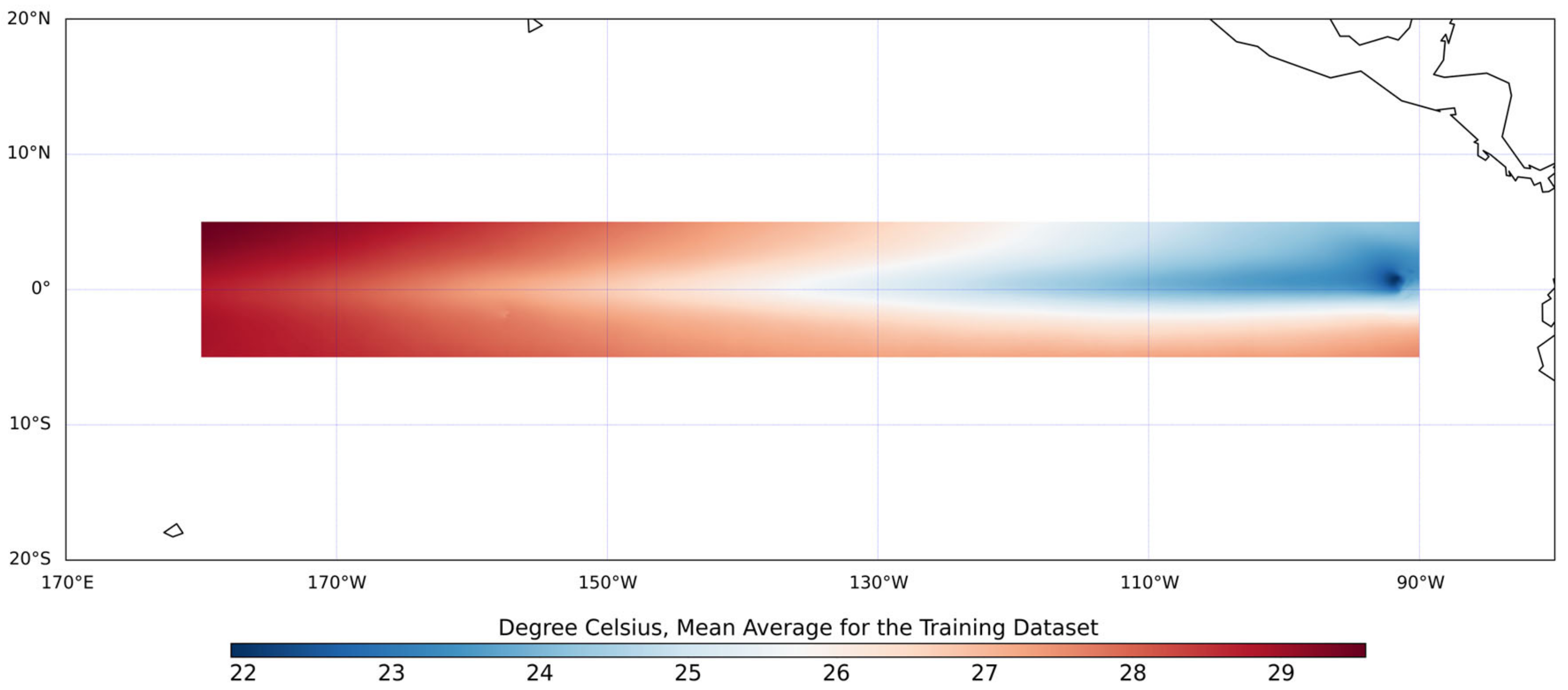
2. Dataset
3. Method
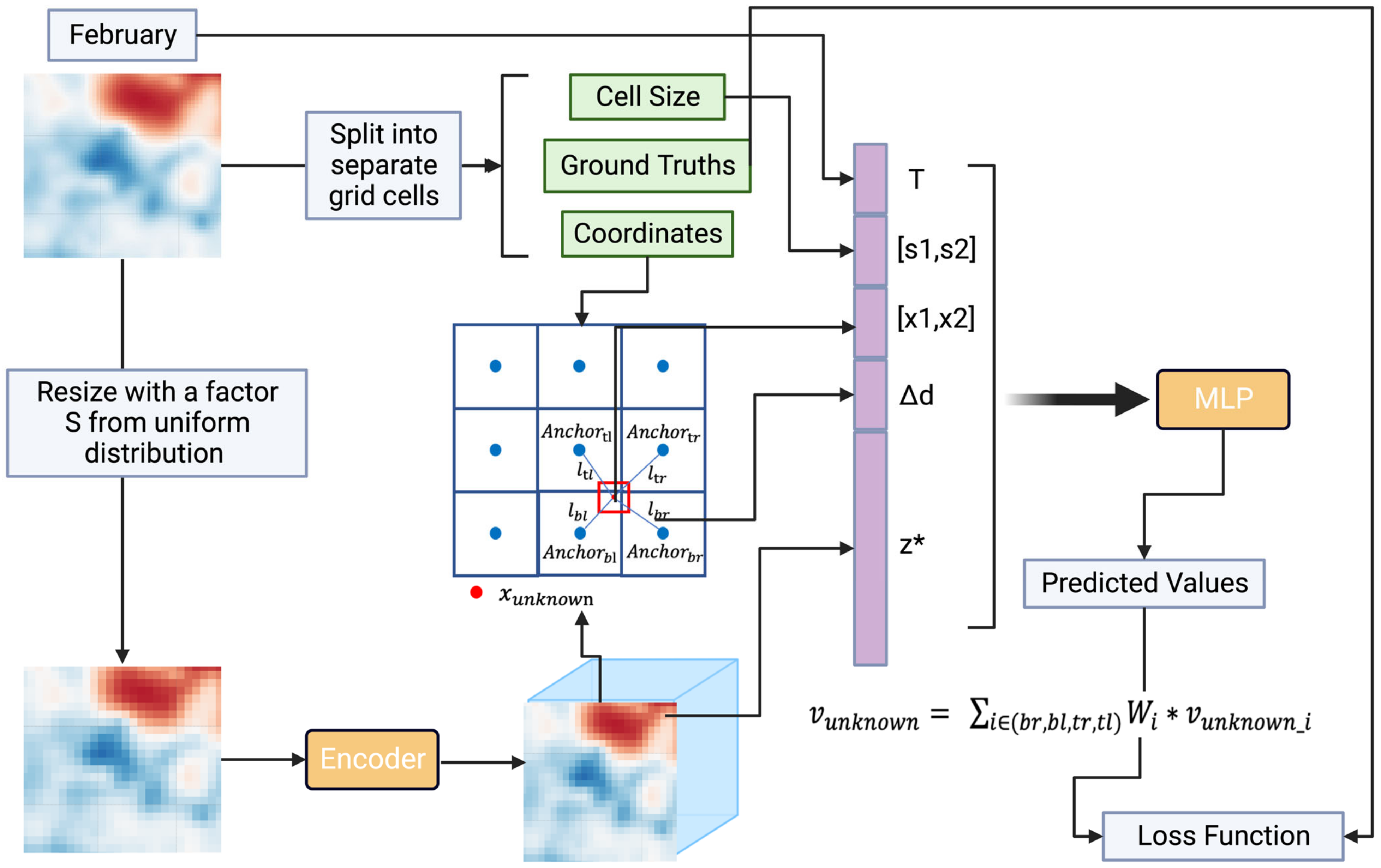
3.1. Overview of Proposed Method
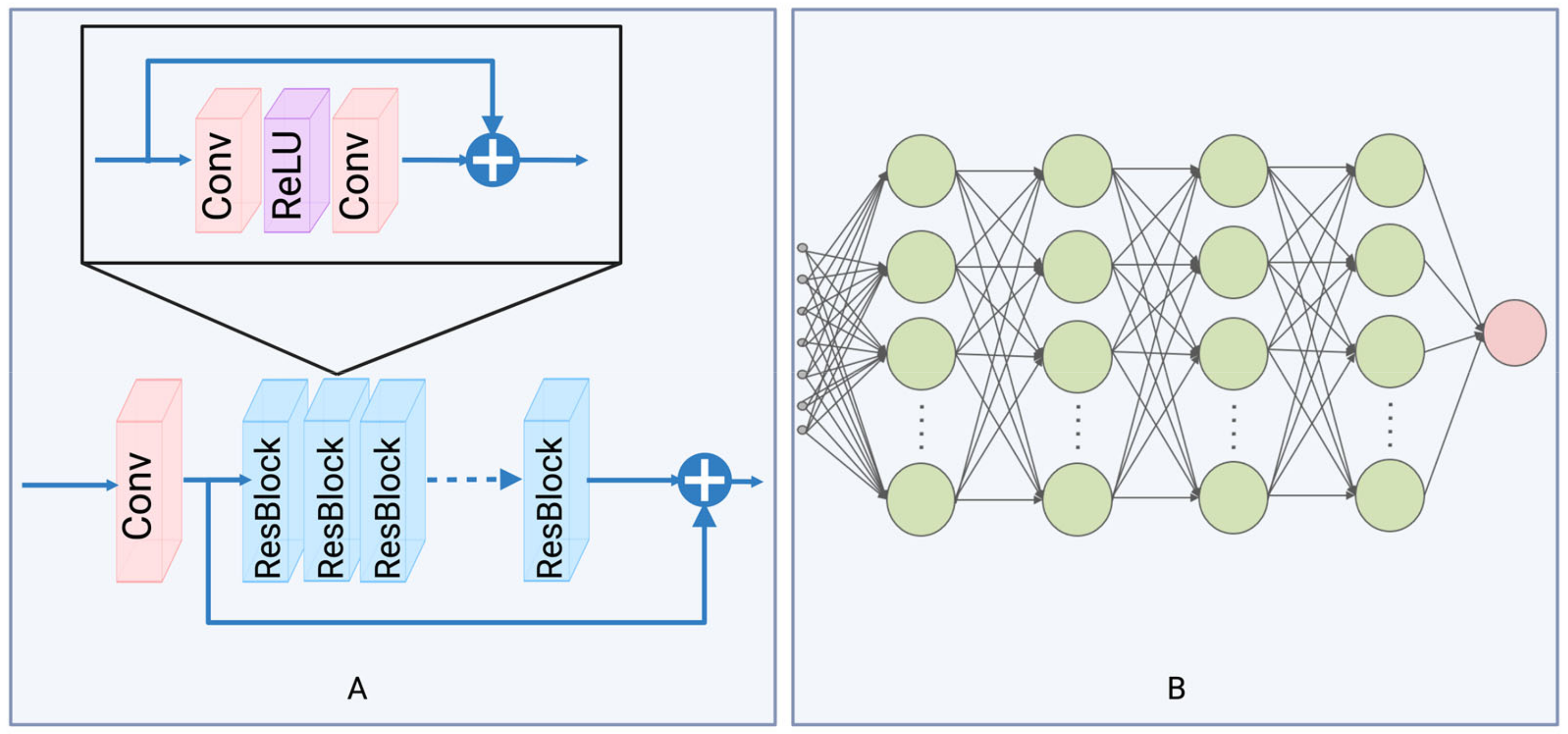
3.2. Enhanced Deep Super-Resolution Network and Multilayer Perceptron
3.3. Implicit Neural-Representation-Based Interpolation with Temporal Information
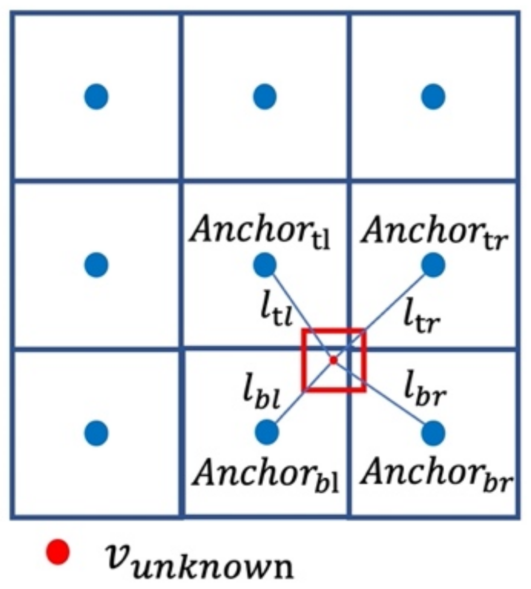
3.3.1. Implicit Neural-Representation-Based Interpolation
3.3.2. Temporal Information Embedding
3.4. Training and Setup
3.5. Validation
4. Results and Discussion
4.1. Comparison of Results Generated by Different Models for Arbitrary Scale HR
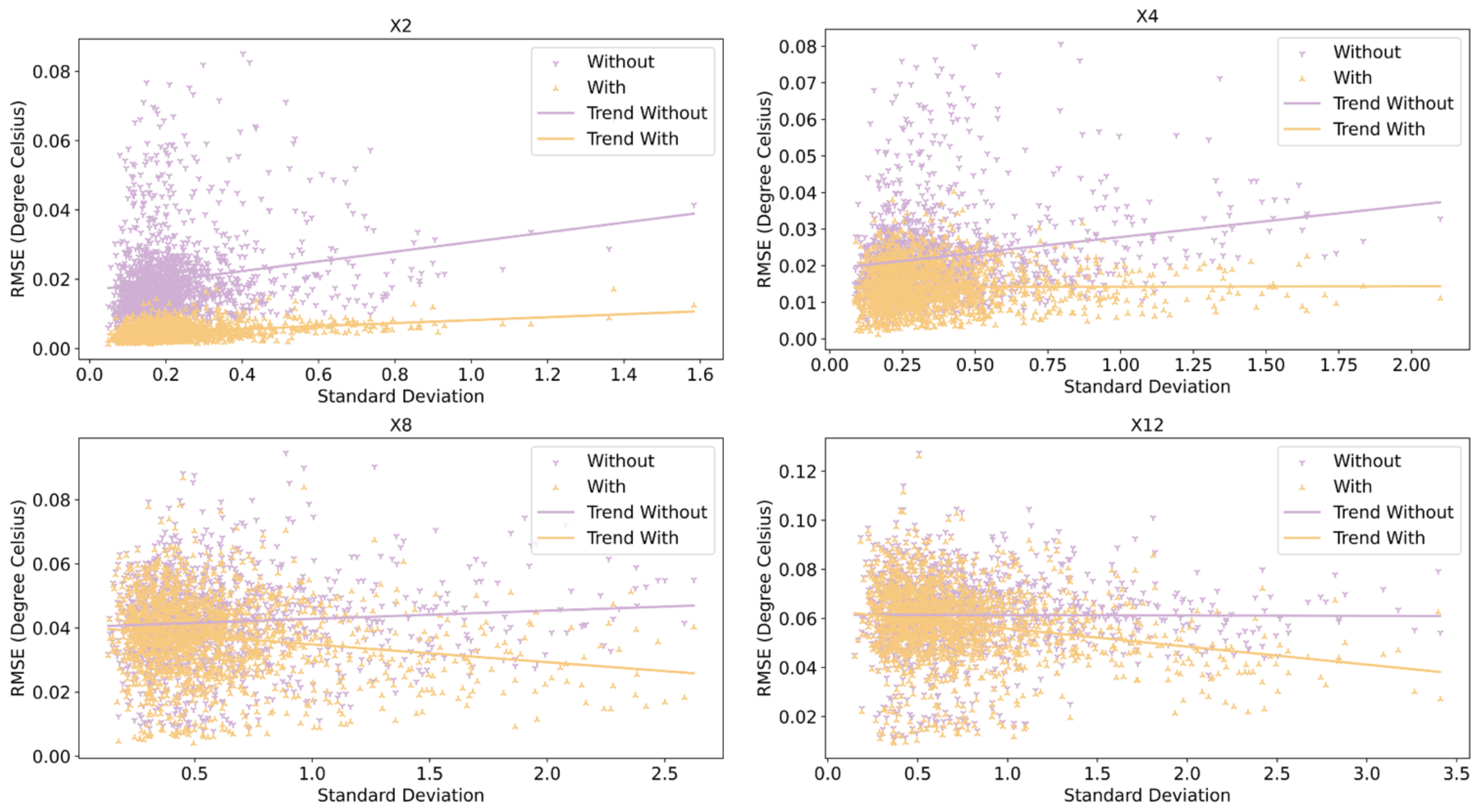
4.2. Analysis of the Impact of Temporal Information
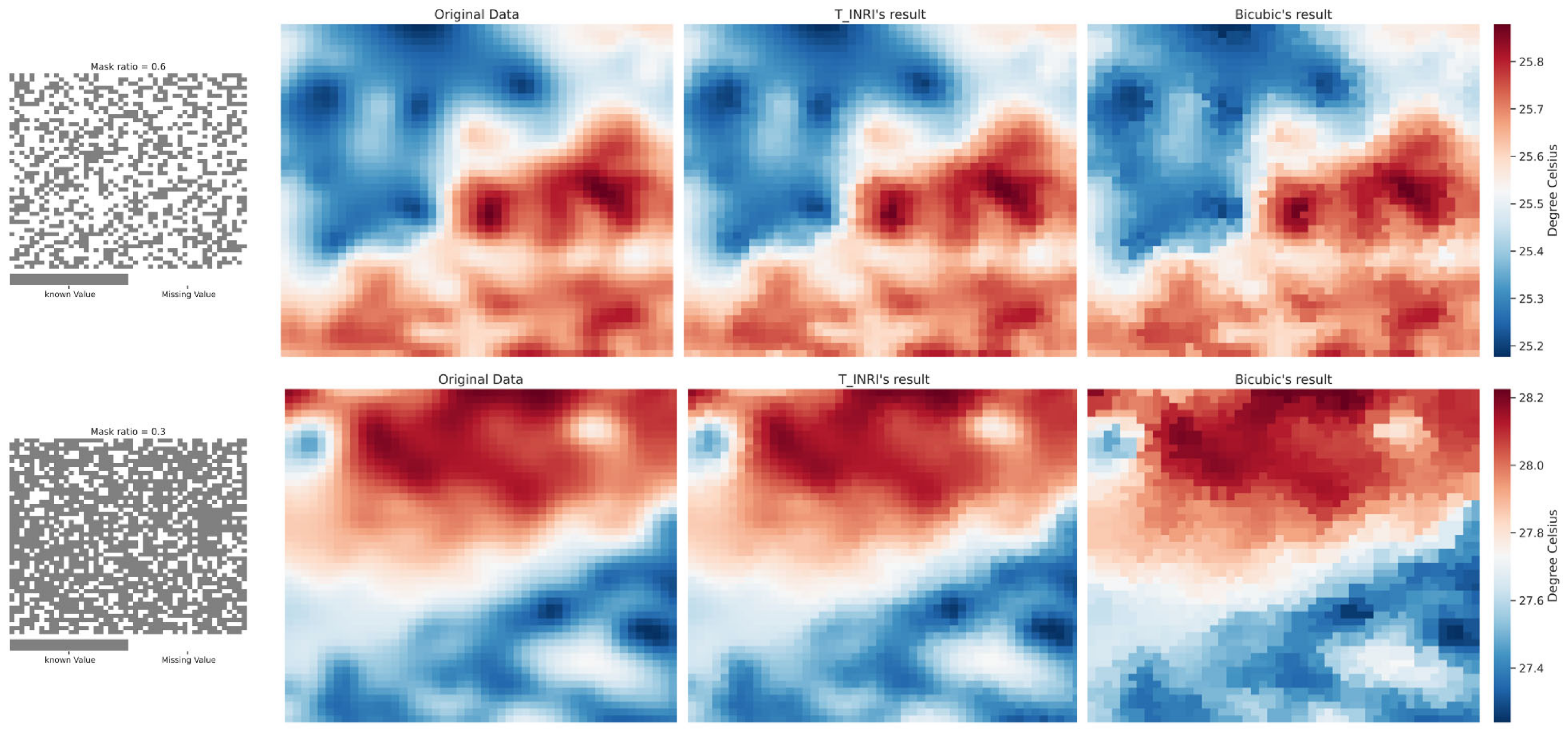
4.3. Analysis of Using Proposed Method for Recovering Missing Value
5. Conclusions
Author Contributions
Funding
Data Availability Statement
Conflicts of Interest
References
- Nigam, S.; Sengupta, A. The Full Extent of El Niño’s Precipitation Influence on the United States and the Americas: The Suboptimality of the Niño 3.4 SST Index. Geophys. Res. Lett. 2021, 48, e2020GL091447. [Google Scholar] [CrossRef]
- Yuan, X.; Kaplan, M.R.; Cane, M.A. The interconnected global climate system-a review of tropical-polar teleconnections. J. Clim. 2018, 31, 5765–5792. [Google Scholar] [CrossRef]
- Burns, J.M.; Subrahmanyam, B. Variability of the Seychelles–Chagos Thermocline Ridge Dynamics in Connection With ENSO and Indian Ocean Dipole. IEEE Geosci. Remote Sens. Lett. 2016, 13, 2019–2023. [Google Scholar] [CrossRef]
- Nouri, N.; Devineni, N.; Were, V.; Khanbilvardi, R. Explaining the trends and variability in the United States tornado records using climate teleconnections and shifts in observational practices. Sci. Rep. 2021, 11, 1741. [Google Scholar] [CrossRef] [PubMed]
- Irannezhad, M.; Liu, J.; Chen, D. Influential Climate Teleconnections for Spatiotemporal Precipitation Variability in the Lancang-Mekong River Basin From 1952 to 2015. J. Geophys. Res. Atmos. 2020, 125, e2020JD033331. [Google Scholar] [CrossRef]
- Gibson, P.B.; Chapman, W.E.; Altinok, A.; Monache, L.D.; DeFlorio, M.J.; Waliser, D.E. Training machine learning models on climate model output yields skillful interpretable seasonal precipitation forecasts. Commun. Earth Environ. 2021, 2, 159. [Google Scholar] [CrossRef]
- Simpson, J.J.; Hufford, G.L.; Fleming, M.D.; Berg, J.S.; Ashton, J.B. Long-term climate patterns in Alaskan surface temperature and precipitation and their biological consequences. IEEE Trans. Geosci. Remote Sens. 2002, 40, 1164–1184. [Google Scholar] [CrossRef]
- Ashok, K.; Behera, S.K.; Rao, S.A.; Weng, H.; Yamagata, T. El Niño Modoki and its possible teleconnection. J. Geophys. Res. Ocean. 2007, 112, 1–27. [Google Scholar] [CrossRef]
- Hernández, J.D.R.; Mesa, Ó.J.; Lall, U. Enso dynamics, trends, and prediction using machine learning. Weather Forecast 2020, 35, 2061–2081. [Google Scholar] [CrossRef]
- Zhang, M.; Rojo-Hernández, J.D.; Yan, L.; Mesa, Ó.J.; Lall, U. Hidden Tropical Pacific Sea Surface Temperature States Reveal Global Predictability for Monthly Precipitation for Sub-Season to Annual Scales. Geophys. Res. Lett. 2022, 49, e2022GL099572. [Google Scholar] [CrossRef]
- Han, D. Comparison of Commonly Used Image Interpolation Methods. In Proceedings of the Conference of the 2nd International Conference on Computer Science and Electronics Engineering (ICCSEE 2013), Hangzhou, China, 22–23 March 2013; pp. 1556–1559. [Google Scholar]
- Vandal, T.; Kodra, E.; Ganguly, S.; Michaelis, A.; Nemani, R.; Ganguly, A.R. Generating high resolution climate change projections through single image super-resolution: An abridged version. In Proceedings of the International Joint Conferences on Artificial Intelligence Organization, Stockholm, Sweden, 13–19 July 2018; Volume 2018, pp. 5389–5395. [Google Scholar]
- Ducournau, A.; Fablet, R. Deep learning for ocean remote sensing: An application of convolutional neural networks for super-resolution on satellite-derived SST data. In Proceedings of the 2016 9th IAPR Workshop on Pattern Recogniton in Remote Sensing (PRRS), Cancun, Mexico, 4 December 2016. [Google Scholar]
- Stengel, K.; Glaws, A.; Hettinger, D.; King, R.N. Adversarial super-resolution of climatological wind and solar data. Proc. Natl. Acad. Sci. USA 2020, 117, 16805–16815. [Google Scholar] [CrossRef] [PubMed]
- Wang, Y.; Karimi, H.A. Generating high-resolution climatological precipitation data using SinGAN. Big Earth Data 2023, 7, 81–100. [Google Scholar] [CrossRef]
- Sitzmann, V.; Lindell, D.B.; Bergman, A.W.; Wetzstein, G. NeurIPS-2020-implicit-neural-representations-with-periodic-activation-functions-Paper. Adv. Neural Inf. Process. Syst. 2020, 33, 7462–7473. [Google Scholar]
- Saragadam, V.; Tan, J.; Balakrishnan, G.; Baraniuk, R.G.; Veeraraghavan, A. MINER: Multiscale Implicit Neural Representation. In Proceedings of the Computer Vision—ECCV 2022, Tel Aviv, Israel, 23–27 October 2022; pp. 318–333. [Google Scholar]
- Peng, S.; Niemeyer, M.; Mescheder, L.; Pollefeys, M.; Geiger, A. Convolutional Occupancy Networks. In Proceedings of the Computer Vision—ECCV 2020: 16th European Conference, Glasgow, UK, 23–28 August 2020; Volume 12348, pp. 523–540. [Google Scholar]
- Sitzmann, V.; Zollhöfer, M.; Wetzstein, G. Scene representation networks: Continuous 3d-structure-aware neural scene representations. Adv. Neural Inf. Process. Syst. 2019, 32, 1–5. [Google Scholar]
- Niemeyer, M.; Mescheder, L.; Oechsle, M.; Geiger, A. Differentiable Volumetric Rendering: Learning Implicit 3D Representations without 3D Supervision. In Proceedings of the IEEE/CVF Conference on Computer Vision and Pattern Recognition, Seattle, WA, USA, 13–19 June 2020; pp. 3501–3512. [Google Scholar]
- Oechsle, M.; Mescheder, L.; Niemeyer, M.; Strauss, T.; Geiger, A. Texture fields: Learning texture representations in function space. In Proceedings of the IEEE/CVF International Conference on Computer Vision, Seoul, Republic of Korea, 27 October–2 November 2019; Volume 2019, pp. 4530–4535. [Google Scholar]
- Shen, L.; Pauly, J.; Xing, L. NeRP: Implicit Neural Representation Learning with Prior Embedding for Sparsely Sampled Image Reconstruction. IEEE Trans. Neural Netw. Learn. Syst. 2022, 1–13. [Google Scholar] [CrossRef] [PubMed]
- Strümpler, Y.; Postels, J.; Yang, R.; Van Gool, L.; Tombari, F. Implicit Neural Representations for Image Compression. In Proceedings of the Computer Vision—ECCV 2022, Tel Aviv, Israel, 23–27 October 2022; pp. 74–91. [Google Scholar]
- Zhang, K.; Zhu, D.; Min, X.; Zhai, G. Implicit Neural Representation Learning for Hyperspectral Image Super-Resolution. IEEE Trans. Geosci. Remote Sens. 2023, 61, 1–5. [Google Scholar] [CrossRef]
- Chen, Z.; Zhang, H. Learning implicit fields for generative shape modeling. In Proceedings of the IEEE/CVF Conference on Computer Vision and Pattern Recognition, Long Beach, CA, USA, 15–20 June 2019; Volume 2019, pp. 5932–5941. [Google Scholar]
- Park, J.J.; Florence, P.; Straub, J.; Newcombe, R.; Lovegrove, S. Deepsdf: Learning continuous signed distance functions for shape representation. In Proceedings of the IEEE/CVF Conference on Computer Vision and Pattern Recognition, Long Beach, CA, USA, 15–20 June 2019; Volume 2019, pp. 165–174. [Google Scholar]
- Chen, Y.; Liu, S.; Wang, X. Learning Continuous Image Representation with Local Implicit Image Function. In Proceedings of the IEEE/CVF Conference on Computer Vision and Pattern Recognition, Nashville, TN, USA, 20–25 June 2021; pp. 8624–8634. [Google Scholar]
- JPL MUR MEaSUREs Project. GHRSST Level 4 MUR Global Foundation Sea Surface Temperature Analysis (v4.1); JPL NASA: Pasadena, CA, USA, 2015. Available online: https://podaac.jpl.nasa.gov/dataset/MUR-JPL-L4-GLOB-v4.1 (accessed on 3 May 2023).
- Chin, T.M.; Vazquez-Cuervo, J.; Armstrong, E.M. A multi-scale high-resolution analysis of global sea surface temperature. Remote Sens. Environ. 2017, 200, 154–169. [Google Scholar] [CrossRef]
- Lim, B.; Son, S.; Kim, H.; Nah, S.; Lee, K.M. Enhanced Deep Residual Networks for Single Image Super-Resolution. In Proceedings of the IEEE Conference on Computer Vision and Pattern Recognition Workshops, Honolulu, HI, USA, 21–26 July 2017; Volume 2017, pp. 1132–1135. [Google Scholar]
- Kim, Y.T.; So, B.J.; Kwon, H.H.; Lall, U. A Multiscale Precipitation Forecasting Framework: Linking Teleconnections and Climate Dipoles to Seasonal and 24-hr Extreme Rainfall Prediction. Geophys. Res. Lett. 2020, 47, e2019GL085418. [Google Scholar] [CrossRef]
- Chen, Z.; Chen, Y.; Liu, J.; Xu, X.; Goel, V.; Wang, Z.; Shi, H.; Wang, X. VideoINR: Learning Video Implicit Neural Representation for Continuous Space-Time Super-Resolution. In Proceedings of the IEEE/CVF Conference on Computer Vision and Pattern Recognition, New Orleans, LA, USA, 18–24 June 2022. [Google Scholar]
- Chen, H.-W.; Xu, Y.-S.; Hong, M.-F.; Tsai, Y.-M.; Kuo, H.-K.; Lee, C.-Y. Cascaded Local Implicit Transformer for Arbitrary-Scale Super-Resolution. In Proceedings of the IEEE/CVF Conference on Computer Vision and Pattern Recognition, Vancouver, BC, Canada, 18–22 June 2023; pp. 18257–18267. [Google Scholar]
- Lee, J.; Jin, K.H. Local Texture Estimator for Implicit Representation Function. In Proceedings of the IEEE/CVF Conference on Computer Vision and Pattern Recognition, New Orleans, LA, USA, 18–24 June 2022; Volume 2022, pp. 1919–1928. [Google Scholar]


| Method | In-Training-Scale RMSE (°C) | Out-of-Training-Scale RMSE (°C) | ||||||||
|---|---|---|---|---|---|---|---|---|---|---|
| 2 | 3 | 4 | 5 | 8 | 10 | 12 | 14 | 16 | 20 | |
| Bicubic | 0.014 | 0.027 | 0.040 | 0.051 | 0.082 | 0.099 | 0.112 | 0.129 | 0.135 | 0.154 |
| Bilinear | 0.014 | 0.027 | 0.039 | 0.050 | 0.079 | 0.095 | 0.107 | 0.124 | 0.130 | 0.148 |
| SRCNN | - | - | 0.015 | - | 0.035 | - | - | - | - | - |
| SRGAN | - | - | 0.014 | - | 0.033 | - | - | - | - | - |
| 0.004 | 0.009 | 0.014 | 0.019 | 0.037 | 0.048 | 0.058 | 0.063 | 0.075 | 0.090 | |
| 0.013 | 0.015 | 0.017 | 0.021 | 0.038 | 0.049 | 0.059 | 0.065 | 0.077 | 0.092 | |
| Method | In-Training-Scale RMSE (°C) | Out-of-Training-Scale RMSE (°C) | ||||||||
|---|---|---|---|---|---|---|---|---|---|---|
| 2 | 3 | 4 | 5 | 8 | 10 | 12 | 14 | 16 | 20 | |
| Bicubic | 0.014 | 0.028 | 0.041 | 0.053 | 0.084 | 0.100 | 0.115 | 0.128 | 0.138 | 0.157 |
| Bilinear | 0.014 | 0.028 | 0.040 | 0.052 | 0.081 | 0.097 | 0.111 | 0.123 | 0.132 | 0.151 |
| 0.005 | 0.010 | 0.015 | 0.020 | 0.038 | 0.050 | 0.060 | 0.069 | 0.077 | 0.092 | |
| 0.014 | 0.021 | 0.023 | 0.028 | 0.044 | 0.055 | 0.064 | 0.073 | 0.081 | 0.096 | |
| Method | Missing Proportion (RMSE (°C)) | ||||||
|---|---|---|---|---|---|---|---|
| 50% | 60% | ||||||
| Bicubic | |||||||
| Linear | |||||||
| Nearest | |||||||
Disclaimer/Publisher’s Note: The statements, opinions and data contained in all publications are solely those of the individual author(s) and contributor(s) and not of MDPI and/or the editor(s). MDPI and/or the editor(s) disclaim responsibility for any injury to people or property resulting from any ideas, methods, instructions or products referred to in the content. |
© 2023 by the authors. Licensee MDPI, Basel, Switzerland. This article is an open access article distributed under the terms and conditions of the Creative Commons Attribution (CC BY) license (https://creativecommons.org/licenses/by/4.0/).
Share and Cite
Wang, Y.; Karimi, H.A.; Jia, X. Reconstruction of Continuous High-Resolution Sea Surface Temperature Data Using Time-Aware Implicit Neural Representation. Remote Sens. 2023, 15, 5646. https://doi.org/10.3390/rs15245646
Wang Y, Karimi HA, Jia X. Reconstruction of Continuous High-Resolution Sea Surface Temperature Data Using Time-Aware Implicit Neural Representation. Remote Sensing. 2023; 15(24):5646. https://doi.org/10.3390/rs15245646
Chicago/Turabian StyleWang, Yang, Hassan A. Karimi, and Xiaowei Jia. 2023. "Reconstruction of Continuous High-Resolution Sea Surface Temperature Data Using Time-Aware Implicit Neural Representation" Remote Sensing 15, no. 24: 5646. https://doi.org/10.3390/rs15245646