
An Integrated Approach for 3D Solar Potential Assessment at the City Scale


Abstract
:
1. Introduction
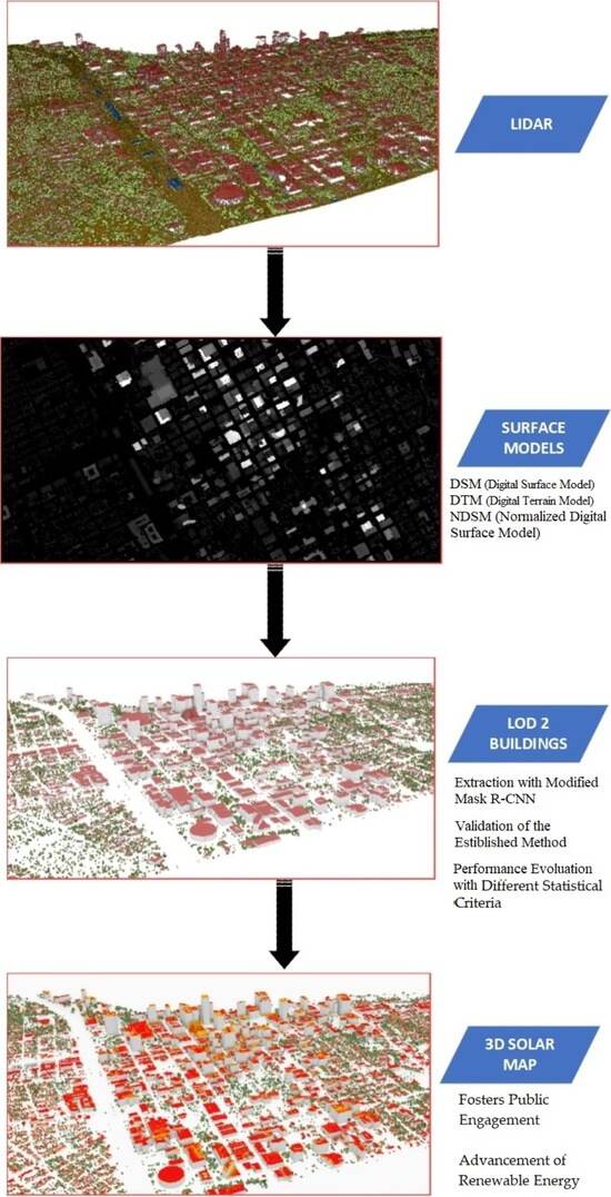
2. Methodology
2.1. Case Study
2.2. LiDAR Dataset
2.2.1. 3D City Model
2.2.2. LOD2 Building Extraction
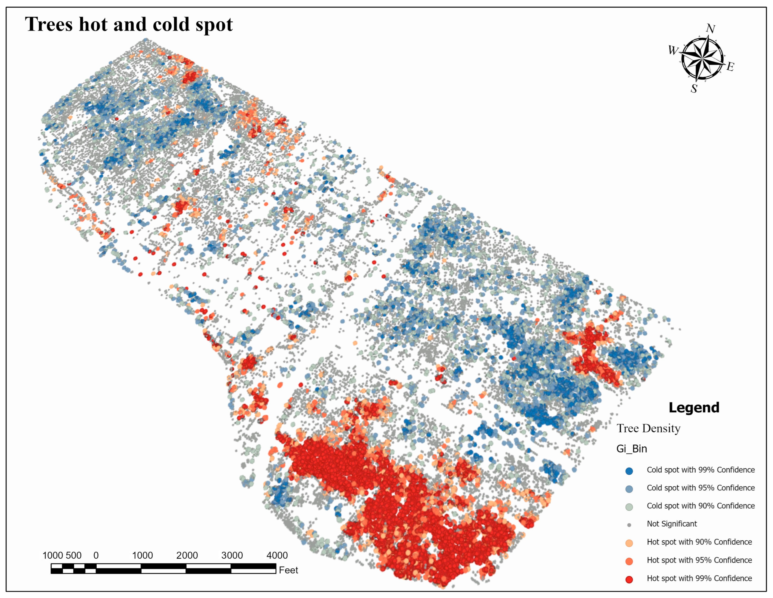
2.2.3. 3D Tree Extraction
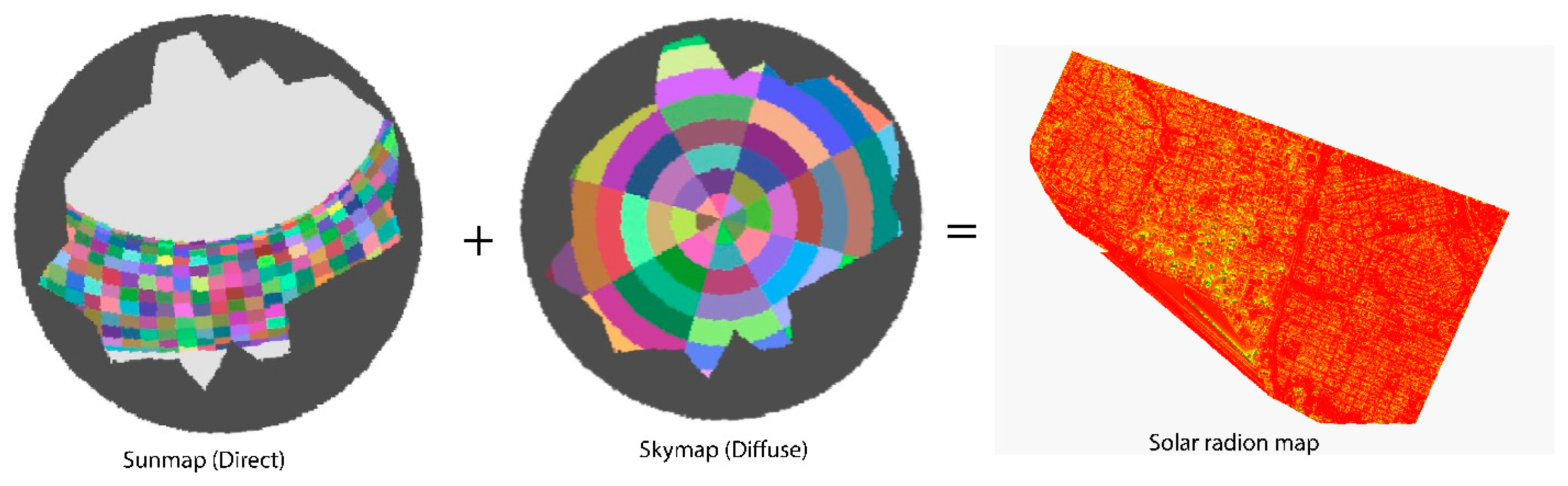
2.3. Solar Irradiation Model
- I.
- without site context (A);
- II.
- with site context (B).
2.4. Evaluating Solar Irradiation with 3D City Model
3. Analysis and Results
3.1. Annual Solar Irradiation Potential Estimation
3.2. Validation
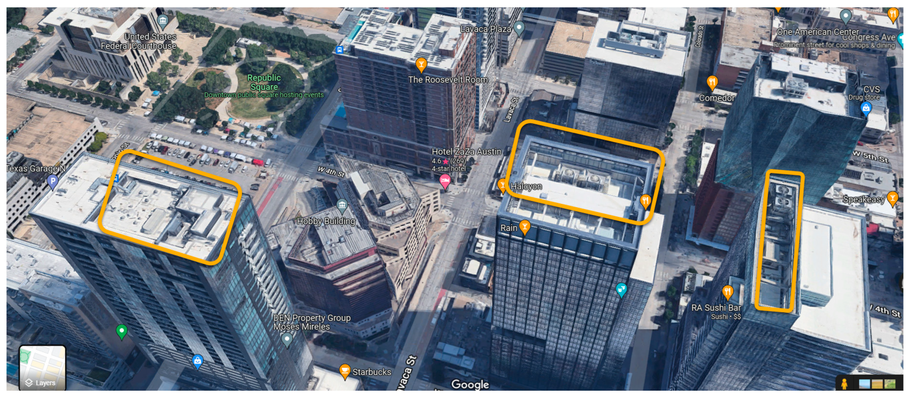
Site Impact Analysis
4. Discussion
5. Conclusions and Future Work
Author Contributions
Funding
Data Availability Statement
Conflicts of Interest
References
- Fogl, M.; Moudrý, V. Influence of vegetation canopies on solar potential in urban environments. Appl. Geogr. 2016, 66, 73–80. [Google Scholar] [CrossRef]
- Devabhaktuni, V.; Alam, M.; Depuru, S.S.S.R.; Green, R.C., II; Nims, D.; Near, C. Solar energy: Trends and enabling technologies. Renew. Sustain. Energy Rev. 2013, 19, 555–564. [Google Scholar] [CrossRef]
- Waqas, H.; Shang, J.; Munir, I.; Ullah, S.; Khan, R.; Tayyab, M.; Mousa, B.G.; Williams, S. Enhancement of the energy performance of an existing building using a parametric approach. J. Energy Eng. 2023, 149, 04022057. [Google Scholar] [CrossRef]
- Jaglin, S. Urban Electric Hybridization: Exploring the Politics of a Just Transition in the Western Cape (South Africa). J. Urban Technol. 2022, 30, 11–33. [Google Scholar] [CrossRef]
- Akaev, A.; Davydova, O. Climate and Energy: Energy Transition Scenarios and Global Temperature Changes Based on Current Technologies and Trends. In Reconsidering the Limits to Growth: A Report to the Russian Association of the Club of Rome; Springer: Cham, Swizterland, 2023; pp. 53–70. [Google Scholar]
- Jing, R.; Liu, J.; Zhang, H.; Zhong, F.; Liu, Y.; Lin, J. Unlock the hidden potential of urban rooftop agrivoltaics energy-food-nexus. Energy 2022, 256, 124626. [Google Scholar] [CrossRef]
- Javanroodi, K.; Nik, V.M.; Mahdavinejad, M. A novel design-based optimization framework for enhancing the energy efficiency of high-rise office buildings in urban areas. Sustain. Cities Soc. 2019, 49, 101597. [Google Scholar] [CrossRef]
- Dong, C.; Nemet, G.; Gao, X.; Barbose, G.; Sigrin, B.; O’shaughnessy, E. Machine learning reduces soft costs for residential solar photovoltaics. Sci. Rep. 2023, 13, 7213. [Google Scholar] [CrossRef] [PubMed]
- Defaix, P.R.; van Sark, W.G.J.H.M.; Worrell, E.; de Visser, E. Technical potential for photovoltaics on buildings in the EU-27. Sol. Energy 2012, 86, 2644–2653. [Google Scholar] [CrossRef]
- Eremia, M.; Toma, L.; Sanduleac, M. The smart city concept in the 21st century. Procedia Eng. 2017, 181, 12–19. [Google Scholar] [CrossRef]
- Lu, Y.; Wu, Z.; Chang, R.; Li, Y. Building Information Modeling (BIM) for green buildings: A critical review and future directions. Autom. Constr. 2017, 83, 134–148. [Google Scholar] [CrossRef]
- Avtar, R.; Tripathi, S.; Aggarwal, A.K.; Kumar, P. Population–urbanization–energy nexus: A review. Resources 2019, 8, 136. [Google Scholar] [CrossRef]
- Hofierka, J.; Kaňuk, J. Assessment of photovoltaic potential in urban areas using open-source solar radiation tools. Renew. Energy 2009, 34, 2206–2214. [Google Scholar] [CrossRef]
- Santos, T.; Gomes, N.; Freire, S.; Brito, M.; Santos, L.; Tenedório, J. Applications of solar mapping in the urban environment. Appl. Geogr. 2014, 51, 48–57. [Google Scholar] [CrossRef]
- Li, Z.; Zhang, Z.; Davey, K. Estimating geographical pv potential using lidar data for buildings in downtown San Francisco. Trans. GIS 2015, 19, 930–963. [Google Scholar] [CrossRef]
- Li, H.; Yi, H. Multilevel governance and deployment of solar PV panels in U.S. cities. Energy Policy 2014, 69, 19–27. [Google Scholar] [CrossRef]
- Srećković, N.; Lukač, N.; Žalik, B.; Štumberger, G. Determining roof surfaces suitable for the installation of PV (photovoltaic) systems, based on LiDAR (Light Detection And Ranging) data, pyranometer measurements, and distribution network configuration. Energy 2016, 96, 404–414. [Google Scholar] [CrossRef]
- Nutkiewicz, A.; Yang, Z.; Jain, R.K. Data-driven Urban Energy Simulation (DUE-S): A framework for integrating engineering simulation and machine learning methods in a multi-scale urban energy modeling workflow. Appl. Energy 2018, 225, 1176–1189. [Google Scholar] [CrossRef]
- Lee, J.; Zlatanova, S. Solar radiation over the urban texture: LIDAR data and image processing techniques for environmental analysis at city scale. In 3D Geo-Information Sciences; Springer: Heidelberg/Berlin, Germany, 2009; pp. 319–340. [Google Scholar]
- Pili, S.; Desogus, G.; Melis, D. A GIS tool for the calculation of solar irradiation on buildings at the urban scale, based on Italian standards. Energy Build. 2018, 158, 629–646. [Google Scholar] [CrossRef]
- Zhang, Y.; Dai, Z.; Wang, W.; Li, X.; Chen, S.; Chen, L. Estimation of the Potential Achievable Solar Energy of the Buildings Using Photogrammetric Mesh Models. Remote Sens. 2021, 13, 2484. [Google Scholar] [CrossRef]
- Hofierka, J.; Gallay, M.; Onačillová, K.; Hofierka, J., Jr. Physically-based land surface temperature modeling in urban areas using a 3-D city model and multispectral satellite data. Urban Clim. 2020, 31, 100566. [Google Scholar] [CrossRef]
- Levinson, R.; Akbari, H.; Pomerantz, M.; Gupta, S. Solar access of residential rooftops in four California cities. Sol. Energy 2009, 83, 2120–2135. [Google Scholar] [CrossRef]
- Tooke, T.R.; Coops, N.C.; Voogt, J.A.; Meitner, M.J. Tree structure influences on rooftop-received solar radiation. Landsc. Urban Plan. 2011, 102, 73–81. [Google Scholar] [CrossRef]
- Machete, R.; Falcão, A.P.; Gomes, M.G.; Rodrigues, A.M. The use of 3D GIS to analyse the influence of urban context on buildings’ solar energy potential. Energy Build. 2018, 177, 290–302. [Google Scholar] [CrossRef]
- Han, Y.; Pan, Y.; Zhao, T.; Sun, C. Evaluating buildings’ solar energy potential concerning urban context based on UAV photogrammetry. In Proceedings of the 16th IBPSA Conference, Rome, Italy, 2–4 September 2019; pp. 3610–3617. [Google Scholar]
- Mansouri Kouhestani, F.; Byrne, J.; Johnson, D.; Spencer, L.; Hazendonk, P.; Brown, B. Evaluating solar energy technical and economic potential on rooftops in an urban setting: The city of Lethbridge, Canada. Int. J. Energy Environ. Eng. 2019, 10, 13–32. [Google Scholar] [CrossRef]
- Huang, X.; Hayashi, K.; Matsumoto, T.; Tao, L.; Huang, Y.; Tomino, Y. Estimation of Rooftop Solar Power Potential by Comparing Solar Radiation Data and Remote Sensing Data—A Case Study in Aichi, Japan. Remote Sens. 2022, 14, 1742. [Google Scholar] [CrossRef]
- Du, Y.; Qin, B.; Zhao, C.; Zhu, Y.; Cao, J.; Ji, Y. A novel spatio-temporal synchronization method of roadside asynchronous mmw radar-camera for sensor fusion. IEEE Trans. Intell. Transp. Syst. 2021, 23, 22278–22289. [Google Scholar] [CrossRef]
- Zhou, G.; Bao, X.; Ye, S.; Wang, H.; Yan, H. Selection of optimal building facade texture images from uav-based multiple oblique image flows. IEEE Trans. Geosci. Remote Sens. 2020, 59, 1534–1552. [Google Scholar] [CrossRef]
- Zhou, G.; Zhou, X.; Song, Y.; Xie, D.; Wang, L.; Yan, G.; Hu, M.; Liu, B.; Shang, W.; Gong, C.; et al. Design of supercontinuum laser hyperspectral light detection and ranging (LiDAR) (SCLaHS LiDAR). Int. J. Remote Sens. 2021, 42, 3731–3755. [Google Scholar] [CrossRef]
- Newman, C.; Edwards, D.; Martek, I.; Lai, J.; Thwala, W.D.; Rillie, I. Industry 4.0 deployment in the construction industry: A bibliometric literature review and UK-based case study. Smart Sustain. Built Environ. 2020, 10, 557–580. [Google Scholar] [CrossRef]
- Prieto, A.; Knaack, U.; Auer, T.; Klein, T. Solar coolfacades: Framework for the integration of solar cooling technologies in the building envelope. Energy 2017, 137, 353–368. [Google Scholar] [CrossRef]
- Sun, R.; Wang, J.; Cheng, Q.; Mao, Y.; Ochieng, W.Y. A new IMU-aided multiple GNSS fault detection and exclusion algorithm for integrated navigation in urban environments. GPS Solut. 2021, 25, 147. [Google Scholar] [CrossRef]
- Gröger, G.; Plümer, L. CityGML–Interoperable semantic 3D city models. ISPRS J. Photogramm. Remote Sens. 2012, 71, 12–33. [Google Scholar] [CrossRef]
- Nys, G.; Billen, R. From consistency to flexibility: A simplified database schema for the management of CityJSON 3D city models. Trans. GIS 2021, 25, 3048–3066. [Google Scholar] [CrossRef]
- Wieland, M.; Nichersu, A.; Murshed, S.M.; Wendel, J. Computing solar radiation on CityGML building data. In Proceedings of the 18th AGILE International Conference on Geographic Information Science, National Harbor, MD, USA, 3–7 August 2015. [Google Scholar]
- Li, X.; Ratti, C. Mapping the spatio-temporal distribution of solar radiation within street canyons of Boston using Google Street View panoramas and building height model. Landsc. Urban Plan. 2019, 191, 103387. [Google Scholar] [CrossRef]
- Gong, F.-Y.; Zeng, Z.-C.; Ng, E.; Norford, L.K. Spatiotemporal patterns of street-level solar radiation estimated using Google Street View in a high-density urban environment. J. Affect. Disord. 2019, 148, 547–566. [Google Scholar] [CrossRef]
- Zhang, X.; Lv, Y.; Tian, J.; Pan, Y. An integrative approach for solar energy potential estimation through 3D modeling of buildings and trees. Can. J. Remote Sens. 2015, 41, 126–134. [Google Scholar] [CrossRef]
- Adjiski, V.; Kaplan, G.; Mijalkovski, S. Assessment of the solar energy potential of rooftops using LiDAR datasets and GIS based approach. Int. J. Eng. Geosci. 2022, 8, 188–199. [Google Scholar] [CrossRef]
- Abd Latif, Z.; Zaki, N.A.M.; Salleh, S.A. GIS-based estimation of rooftop solar photovoltaic potential using LiDAR. In Proceedings of the 2012 IEEE 8th International Colloquium on Signal Processing and Its Applications, Malacca, Malaysia, 23–25 March 2012; pp. 388–392. [Google Scholar]
- Taminiau, J.; Byrne, J.; Kim, J.; Kim, M.; Seo, J. Inferential-and measurement-based methods to estimate rooftop “solar city” potential in megacity Seoul, South Korea. Wiley Interdiscip. Rev. Energy Environ. 2022, 11, e438. [Google Scholar] [CrossRef]
- Jakica, N. State-of-the-art review of solar design tools and methods for assessing daylighting and solar potential for building-integrated photovoltaics. Renew. Sustain. Energy Rev. 2018, 81, 1296–1328. [Google Scholar] [CrossRef]
- Hofierka, J.; Zlocha, M. A new 3-D solar radiation model for 3-D city models. Trans. GIS 2012, 16, 681–690. [Google Scholar] [CrossRef]
- Feijoo, F.; Iyer, G.C.; Avraam, C.; Siddiqui, S.A.; Clarke, L.E.; Sankaranarayanan, S.; Binsted, M.T.; Patel, P.L.; Prates, N.C.; Torres-Alfaro, E.; et al. The future of natural gas infrastructure development in the United states. Appl. Energy 2018, 228, 149–166. [Google Scholar] [CrossRef]
- Lei, R.; Feng, S.; Lauvaux, T. Country-scale trends in air pollution and fossil fuel CO2 emissions during 2001–2018: Confronting the roles of national policies and economic growth. Environ. Res. Lett. 2020, 16, 014006. [Google Scholar] [CrossRef]
- Upadhyay, R.K. Markers for global climate change and its impact on social, biological and ecological systems: A review. Am. J. Clim. Chang. 2020, 09, 159–203. [Google Scholar] [CrossRef]
- Yu, J.; Tang, Y.M.; Chau, K.Y.; Nazar, R.; Ali, S.; Iqbal, W. Role of solar-based renewable energy in mitigating CO2 emissions: Evidence from quantile-on-quantile estimation. Renew. Energy 2022, 182, 216–226. [Google Scholar] [CrossRef]
- Kutzner, T.; Chaturvedi, K.; Kolbe, T.H. CityGML 3.0: New functions open up new applications. PFG–J. Photogramm. Remote Sens. Geoinf. Sci. 2020, 88, 43–61. [Google Scholar] [CrossRef]
- Biljecki, F.; Ledoux, H.; Stoter, J. Does a finer level of detail of a 3D city model bring an improvement for estimating shadows. In Advances in 3D Geoinformation; Springer: Heidelberg/Berlin, Germany, 2017; pp. 31–47. [Google Scholar]
- Dukai, B.; Ledoux, H.; Stoter, J.E. A multi-height LoD1 model of all buildings in the Netherlands. ISPRS Ann. Photogramm. Remote Sens. Spat. Inf. Sci. 2019, 4, 51–57. [Google Scholar] [CrossRef]
- Pijl, A.; Bailly, J.-S.; Feurer, D.; El Maaoui, M.A.; Boussema, M.R.; Tarolli, P. TERRA: Terrain extraction from elevation rasters through repetitive anisotropic filtering. Int. J. Appl. Earth Obs. Geoinf. 2020, 84, 101977. [Google Scholar] [CrossRef]
- Shabbir, A.; Ali, N.; Ahmed, J.; Zafar, B.; Rasheed, A.; Sajid, M.; Ahmed, A.; Dar, S.H. Satellite and scene image classification based on transfer learning and fine tuning of ResNet50. Math. Probl. Eng. 2021, 2021, 5843816. [Google Scholar] [CrossRef]
- Zhao, K.; Kang, J.; Jung, J.; Sohn, G. Building extraction from satellite images using mask R-CNN with building boundary regularization. In Proceedings of the IEEE Computer Society Conference on Computer Vision and Pattern Recognition Workshops, Salt Lake City, UT, USA, 18–22 June 2018; pp. 247–251. [Google Scholar]
- Maharana, K.; Mondal, S.; Nemade, B. A review: Data pre-processing and data augmentation techniques. Glob. Transit. Proc. 2022, 3, 91–99. [Google Scholar] [CrossRef]
- Sakeena, M.; Stumpe, E.; Despotovic, M.; Koch, D.; Zeppelzauer, M. On the Robustness and Generalization Ability of Building Footprint Extraction on the Example of SegNet and Mask R-CNN. Remote Sens. 2023, 15, 2135. [Google Scholar] [CrossRef]
- Nath, N.D.; Chaspari, T.; Behzadan, A.H. Single- and multi-label classification of construction objects using deep transfer learning methods. J. Inf. Technol. Constr. 2019, 24, 511–526. [Google Scholar] [CrossRef]
- Gupta, S.; Weinacker, H.; Koch, B. Comparative analysis of clustering-based approaches for 3-d single tree detection using airborne fullwave lidar data. Remote Sens. 2010, 2, 968–989. [Google Scholar] [CrossRef]
- Liang, J.; Gong, J.; Zhou, J.; Ibrahim, A.N.; Li, M. An open-source 3D solar radiation model integrated with a 3D Geographic Information System. Environ. Model. Softw. 2015, 64, 94–101. [Google Scholar] [CrossRef]
- Bode, C.A.; Limm, M.P.; Power, M.E.; Finlay, J.C. Subcanopy Solar Radiation model: Predicting solar radiation across a heavily vegetated landscape using LiDAR and GIS solar radiation models. Remote Sens. Environ. 2014, 154, 387–397. [Google Scholar] [CrossRef]
- Massimo, A.; Dell’Isola, M.; Frattolillo, A.; Ficco, G. Development of a geographical information system (GIS) for the integration of solar energy in the energy planning of a wide area. Sustainability 2014, 6, 5730–5744. [Google Scholar] [CrossRef]
- Fu, P.; Rich, P.M. Design and Implementation of the Solar Analyst: An ArcView Extension for Modeling Solar Radiation at Landscape Scales. In Proceedings of the 1999 Esri User Conference Proceedings, San Diego, CA, USA, 27–30 July 1999; pp. 1–24. [Google Scholar]
- Kausika, B.B.; van Sark, W.G.J.H.M. Calibration and validation of ArcGIS solar radiation tool for photovoltaic potential determination in the Netherlands. Energies 2021, 14, 1865. [Google Scholar] [CrossRef]
- Quirós, E.; Pozo, M.; Ceballos, J. Solar potential of rooftops in Cáceres city, Spain. J. Maps 2018, 14, 44–51. [Google Scholar] [CrossRef]
- Rich, P.M. Characterizing plant canopies with hemispherical photographs. Remote Sens. Rev. 1990, 5, 3–29. [Google Scholar] [CrossRef]
- Enjavi-Arsanjani, M.; Hirbodi, K.; Yaghoubi, M. Solar energy potential and performance assessment of CSP plants in different areas of Iran. Energy Procedia. 2015, 69, 2039–2048. [Google Scholar] [CrossRef]
- Orte, F.; Lusi, A.; Carmona, F.; D’Elia, R.; Faramiñán, A.; Wolfram, E. Comparison of NASA-POWER solar radiation data with ground-based measurements in the south of South America. In Proceedings of the 2021 XIX Workshop on Information Processing and Control (RPIC), San Juan, Argentina, 3–5 November 2021; pp. 1–4. [Google Scholar]
- Teyabeen, A.A.; Elhatmi, N.B.; Essnid, A.A.; Mohamed, F. Estimation of monthly global solar radiation over twelve major cities of Libya. Energy Built Environ. 2022, 5, 46–57. [Google Scholar] [CrossRef]
- Kowe, P.; Mutanga, O.; Odindi, J.; Dube, T. Exploring the spatial patterns of vegetation fragmentation using local spatial autocorrelation indices. J. Appl. Remote Sens. 2019, 13, 024523. [Google Scholar] [CrossRef]
- Getis, A.; Ord, J.K. The analysis of spatial association by use of distance statistics. In Perspectives on Spatial Data Analysis; Springer: Berlin/Heidelberg, Germany, 2010; pp. 127–145. [Google Scholar]
- Brito, M.C.; Redweik, P.; Catita, C.; Freitas, S.; Santos, M. 3D solar potential in the urban environment: A case study in Lisbon. Energies 2019, 12, 3457. [Google Scholar] [CrossRef]
- Lobaccaro, G.; Croce, S.; Vettorato, D.; Carlucci, S. A holistic approach to assess the exploitation of renewable energy sources for design interventions in the early design phases. Energy Build. 2018, 175, 235–256. [Google Scholar] [CrossRef]
- Prieto, I.; Izkara, J.L.; Usobiaga, E. The application of LiDAR data for the solar potential analysis based on urban 3D model. Remote Sens. 2019, 11, 2348. [Google Scholar] [CrossRef]
- Sredenšek, K.; Štumberger, B.; Hadžiselimović, M.; Mavsar, P.; Seme, S. Physical, geographical, technical, and economic potential for the optimal configuration of photovoltaic systems using a digital surface model and optimization method. Energy 2022, 242, 122971. [Google Scholar] [CrossRef]
- Allen, A.; Henze, G.; Baker, K.; Pavlak, G. Evaluation of low-exergy heating and cooling systems and topology optimization for deep energy savings at the urban district level. Energy Convers. Manag. 2020, 222, 113106. [Google Scholar] [CrossRef]
- Zhong, Q.; Nelson, J.R.; Tong, D.; Grubesic, T.H. A spatial optimization approach to increase the accuracy of rooftop solar energy assessments. Appl. Energy 2022, 316, 119128. [Google Scholar] [CrossRef]
- Brito, M.; Freitas, S.; Guimarães, S.; Catita, C.; Redweik, P. The importance of facades for the solar PV potential of a Mediterranean city using LiDAR data. Renew. Energy 2017, 111, 85–94. [Google Scholar] [CrossRef]
- Lindberg, F.; Jonsson, P.; Honjo, T.; Wästberg, D. Solar energy on building envelopes—3D modelling in a 2D environment. Sol. Energy 2015, 115, 369–378. [Google Scholar] [CrossRef]


| Attribute | Value |
|---|---|
| Source | https://data.tnris.org/?pg=1&inc=24#5.5/31.33/-99.341 (accessed on 23 November 2021) |
| Dataset Name | LiDAR Austin East/West/SW-2017 50 cm-central-Texas |
| Derived Maps | Aerial imaging, cadastral, and land parcel |
| Collection Timeframe | 28 January 2017 through 22 March 2017 |
| Spatial Reference | Transverse Mercator (UTM) Zone 14N |
| Classified pointcloud with Class Codes | 1 = unclassified, 2 = bare earth ground, 3 = low vegetation, 4 = medium vegetation, 5 = high vegetation, 6 = buildings, 7 = low point/noise, 9 = water, 10 = ignored ground ((1 × NPS) near BL), 13 = bridges, 14 = culverts |
| Collection Area | 5804 sq mi |
| Linear Unit | meter |
| Flight Lines | 457 (434 flight lines, 16 cross-ties, and 7 filler lines) |
| Vertical Spatial Reference | North American Vertical Datum 1988 (NAVD88), Geoid 12b |
| Sensor Type | Riegl R680i |
| Camera Serial Numbers | Unit 165, 863, 216 |
| Vertical Accuracy (NVA Checkpoints) | RMSE 5.35, 95% Percentile 11.248 cm |
| Vegetated Vertical Accuracy (VVA) | RMSE 5.496, 95% Percentile 10.700 cm |
| Nominal Post Spacing (NPS) | 0.50 m |
| Scan Angle | 60 degrees |
| Average Ground Speed | 127 Knts (flight speed) |
| Laser Pulse Rate | 330 kHz |
| Scan Rate | 130 Hz |
| Average Flying Altitude | 2869 ft above mean terrain (AMT) |
| Aggregated Nominal Point Spacing (ANPS) | 0.48 m |
| Aggregated Nominal Point Density (ANPD) | 4.39 pts/m2 |
| Confidence Level (%) | Gi_Bin | Pattern | Tree Spots | Tree Density |
|---|---|---|---|---|
| 99 | 3 | VH | hotspot | VH |
| clustered | Tall Trees | |||
| −3 | VH | coldspot | VL | |
| clustered | Tall Trees | |||
| 95 | 2 | M clustered | hotspot | MH |
| Tall Trees | ||||
| −2 | M clustered | coldspot | ML | |
| Tall Trees | ||||
| 90 | 1 | Clustered | hotspot | H |
| Tall Trees | ||||
| −1 | Clustered | coldspot | L | |
| Tall Trees |
Disclaimer/Publisher’s Note: The statements, opinions and data contained in all publications are solely those of the individual author(s) and contributor(s) and not of MDPI and/or the editor(s). MDPI and/or the editor(s) disclaim responsibility for any injury to people or property resulting from any ideas, methods, instructions or products referred to in the content. |
© 2023 by the authors. Licensee MDPI, Basel, Switzerland. This article is an open access article distributed under the terms and conditions of the Creative Commons Attribution (CC BY) license (https://creativecommons.org/licenses/by/4.0/).
Share and Cite
Waqas, H.; Jiang, Y.; Shang, J.; Munir, I.; Khan, F.U. An Integrated Approach for 3D Solar Potential Assessment at the City Scale. Remote Sens. 2023, 15, 5616. https://doi.org/10.3390/rs15235616
Waqas H, Jiang Y, Shang J, Munir I, Khan FU. An Integrated Approach for 3D Solar Potential Assessment at the City Scale. Remote Sensing. 2023; 15(23):5616. https://doi.org/10.3390/rs15235616
Chicago/Turabian StyleWaqas, Hassan, Yuhong Jiang, Jianga Shang, Iqra Munir, and Fahad Ullah Khan. 2023. "An Integrated Approach for 3D Solar Potential Assessment at the City Scale" Remote Sensing 15, no. 23: 5616. https://doi.org/10.3390/rs15235616