1. Introduction
Synthetic aperture radar (SAR) is one of the main means in the field of remote sensing because of its all-day and all-weather imaging characteristics [
1]. Polarization is an important attribute of electromagnetic waves. With the development of sensor technology, the SAR imaging mode has been extended from single polarization to full polarization. Applying all polarization information to the SAR system constitutes the polarimetric SAR (PolSAR) system. Compared with SAR, PolSAR can provide complete target electromagnetic scattering characteristics and polarization information [
2]. Ship detection has been a research hotspot in the fields of SAR and PolSAR applications, which helps to strengthen maritime traffic management and has good application prospects in civilian and military fields, such as safeguarding maritime rights and improving maritime warning capabilities.
Since ship targets are generally active in the vast ocean, they have position uncertainty and target dispersion. In addition, the massive remote sensing data used for ship detection include a large number of land areas and seawater areas without ships. Therefore, how to quickly and easily locate the area where ships exist in a complete remote sensing image through a ship coarse detection method, that is, extracting the potential areas of ships, is an important issue in ship detection tasks in massive remote sensing data. Another role of ship potential area extraction is to reduce the complexity of computation for polarimetric feature extraction in PolSAR ship detection tasks. In order to better extract the spatial and polarimetric features of PolSAR images and improve the detection effect, the latest PolSAR ship detection method based on deep learning [
3] uses multiple polarimetric feature extraction methods to construct multi-channel data as input for deep learning networks. If polarimetric feature extraction is performed on the entire scene image, the computational complexity will be significant. Therefore, it is a feasible method to reduce the computational complexity by only calculating the polarimetric features of the potential areas through ship potential area extraction.
Currently, three types of methods for PolSAR ship potential area extraction, also known as ship coarse detection, are as follows: (1) Statistical distribution-based methods—since ship detection is looking for a specific target from the ocean background and ship targets have strong scattered echoes compared to sea clutter, ships can be detected by modeling sea clutter and searching for outliers through a statistical analysis. The Constant False-Alarm Rate (CFAR) method and its variants [
4] belong to this category. The core of CFAR methods is to model sea clutter more accurately, e.g., Liu et al. [
5] applied an adaptive truncation method to estimate the parameters of the statistical models in PolSAR images. (2) Polarimetric scattering-feature-based methods, including various polarization decomposition methods [
6,
7,
8,
9,
10]—in a PolSAR target detection task, Bordbari et al. [
11] categorized the scattering mechanism into target and non-target and used subspace projection to improve the detection performance. (3) Spatial-feature-based methods—spatial-feature-based methods use manually designed or automatically learned features extracted in the spatial domain to distinguish ships from the background. Grandi et al. [
12] used wavelet features to detect targets in PolSAR images, which explains the dependence of texture measurements on the polarization state. All of the above ship potential area extraction methods have some limitations. On the one hand, CFAR-type methods usually need to perform an accurate sea–land segmentation first to ensure that the background is seawater. Although current methods based on GIS information can quickly and efficiently exclude large land areas, the fine segmentation at the sea–land boundaries still relies on specially designed sea–land segmentation methods. In addition, the non-homogeneous sea clutter under a complex sea state makes it difficult to model the clutter distribution uniformly on the whole PolSAR image. On the other hand, PolSAR ship potential area extraction methods based on polarimetric features as well as spatial features rely on the accurate description of the features. The backscattering from radar targets is sensitive to the relative geometric relationship between the target attitude and the radar line of sight, which leads to scattering diversity of the target [
13,
14], and the scattering diversity makes the polarimetric and spatial features of the ship variable, which makes it difficult to detect based on the pixel-level features. In addition, complex sea surface backgrounds, including islands, waves, ship wakes, defocusing, azimuth ambiguity, cross sidelobes, stripe noise, strong scattering artificial targets (e.g., lighthouses and buoys), etc., can interfere with the detection of ship targets in the case of imperfect feature descriptions, resulting in false alarms and missed alarms. The visualization of some false alarms is shown in
Figure 1.
We designed a method for the PolSAR ship potential area extraction task, so that it can be applied to both the nearshore areas containing part of the land and the distant sea areas, and it can coarsely detect ships while excluding the interference of complex backgrounds without relying on the fine land–sea segmentation algorithms other than GIS information. Under the premise that extracting traditional pixel-level features is not effective, trying to use the latent high-level semantic information in PolSAR images is a good idea to solve the problem. The bag-of-words (BOW) models and the topic models were initially used for text data mining and natural language processing (NLP), which can extract the semantic information, especially latent topic information, in documents. They can also be applied in the field of remote sensing image processing if the images or image blocks are regarded as the documents or bag of words [
15]. Sivic et al. [
16] introduced the bag-of-words model for the first time in the field of computer vision. The visual bag-of-words model treats an image as a set of local visual features within a bag and ignores the spatial layout information of the features. It borrows the idea of the traditional bag-of-words model, which treats the features extracted from an image as visual words and ignores the order of occurrence and grammatical structure of the words. By statistically modeling visual words, the features are reduced in dimensionality. For the case that multiple visual features correspond to a visual word, Yuan et al. [
17] proposed a meaningful spatially co-occurrent pattern of visual words to eliminate the influence of polysemous visual words. For the topic model, Deerwester et al. [
18] proposed the latent semantic analysis (LSA) model. Later, Hofmann [
19] extended it to Probabilistic LSA (pLSA). Bosch et al. [
20] regarded image classes as latent topics, using the pLSA method to automatically obtain these latent topics from bag-of-words features of images for classification. The Latent Dirichlet Allocation (LDA) model [
21] is also a classic generative topic model, which introduces parameters that follow the Dirichlet distribution on the basis of pLSA to establish the probability distribution of the latent topic variable. Li et al. [
22] used the LDA model for scene classification for the first time, while Zhong et al. [
23] utilized an improved LDA topic model for natural image classification. There are the following problems to be solved when using the LDA topic model for PolSAR ship potential area extraction: Firstly, the bag-of-words generation method should be optimized, so that each bag of words contains homogeneous features as much as possible to facilitate the subsequent semantic information extraction. Secondly, the original PolSAR image has a large height and width, and when there are too many pixels, the LDA topic model has large computational complexity, so measures need to be taken to reduce the computational complexity. Thirdly, some of the targets with similar semantic features are not actually homogeneous targets, and further precise differentiation between them is needed to improve the precision rate as much as possible on the basis of ensuring a high recall rate for ship coarse detection.
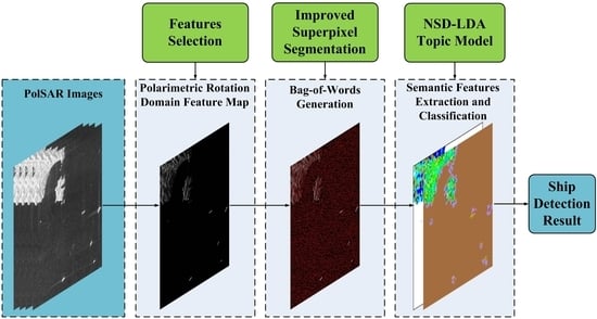
In this article, we propose a PolSAR ship potential area extraction (coarse detection) method based on neighborhood semantic differences of the LDA bag-of-words topic model (NSD-LDA). Firstly, in order to reduce the effect of scattering diversity, the unified polarimetric rotation domain theory proposed by Chen et al. [
24,
25,
26] is introduced. By selecting several typical polarimetric rotation domain feature parameters, a feature map suitable for extracting high-level semantic features is obtained, which not only maximizes the differences between the target and the background but also maximizes prior homogeneous regions to reduce the computational complexity of the subsequent semantic feature extraction. Secondly, we generate the bag of words via an improved superpixel segmentation method. The traditional superpixel segmentation method is not applicable to the selected feature maps, and a more suitable superpixel segmentation method can be obtained by improving the seed point selection, iteration strategy, and termination conditions. Then, on the bag of words obtained with the superpixel segmentation method, high-level semantic information is extracted using our proposed NSD-LDA method. Specifically, in order to enhance the correlation between polarimetric and spatial features, making the extracted high-level semantic information more accurate, on the basis of generating the bag of words using the superpixel method, the differences between the semantic vectors of the target bag of words and its neighboring bags of words are used to replace the original target semantic vectors as the extracted high-level semantic features. Finally, based on the extracted high-level semantic features, the PolSAR ship potential area extraction (coarse detection) is completed using an SVM classifier, prior knowledge, and morphological post-processing. The main contributions of this article are summarized as follows:
We propose an unsupervised PolSAR ship potential area extraction (coarse detection) method, which can effectively migrate images obtained from the same type of sensors and facilitate deployment on large-scale production lines.
By extracting high-level semantic features of the generated bag of words, our method has better applicability to complex backgrounds including parts of land.
Through polarimetric rotation domain feature selection, improved superpixel bag-of-words generation, and high-level semantic features extraction, our method further strengthens the correlation between polarimetric and spatial features, resulting in more robust ship detection results.
The innovations of our method are summarized as follows:
By selecting polarimetric rotation domain feature parameters under dual-constraint conditions, we improved the discrimination between the target and background while expanding prior homogeneous semantic regions, and obtained polarimetric feature maps suitable for subsequent bag-of-words generation and high-level semantic feature extraction.
By improving the superpixel segmentation method and using prior information guidance, the bag of words applicable to the selected polarimetric feature map is constructed, which combines polarimetric features with spatial features and significantly reduces the computational complexity of the subsequent semantic feature extraction.
With the proposed NSD-LDA method, polarimetric and spatial features are more correlated, and the extracted potential areas of ships are more accurate.
The remainder of this paper is organized as follows: The proposed method is de-tailed in
Section 2, followed by experimental results in
Section 3. Some discussions are presented in
Section 4, and
Section 5 concludes the paper.
2. Methods
In this paper, we propose a PolSAR ship potential area extraction method based on neighborhood semantic differences of an LDA bag-of-words topic model. A flowchart of this method is given in
Figure 2. Firstly, several polarimetric rotation domain feature parameters are extracted from the original PolSAR image and compared for selection, and the feature parameters are selected to construct a polarimetric feature map containing polarimetric information based on the maximization of the difference between the ship target and the background and the maximization of the number of pixels in the prior homogeneous region (seawater). Details will be presented in
Section 2.1. Secondly, the selected polarimetric feature map is clustered to generate a bag of words by using an improved superpixel method. All details are discussed at length in
Section 2.2. Thirdly, the high-level semantic information is extracted with the proposed NSD-LDA method for each bag of words. This part will be discussed thoroughly in
Section 2.3. Finally, the extracted semantic information is classified using the SVM classifier and then post-processed using expert knowledge to obtain the results of ship potential area extraction. This part will be presented in
Section 2.4.
2.1. Polarimetric Rotation Domain Features Selection
2.1.1. Characterization of Polarimetric Rotation Domain Feature Parameters
The scattering diversity of radar targets makes SAR/PolSAR information processing more difficult. In order to explore and utilize the information contained in this scattering diversity, Chen et al. extended the polarimetric information obtained under specific imaging geometric relations to the direction rotating around the radar line of sight, and they proposed a unified polarimetric rotation domain theory [
24] and polarimetric correlation/coherence feature rotation domain interpretation tools [
25,
26].
Specifically, for PolSAR images, the polarimetric scattering matrix
can be represented as follows under horizontal (
) and vertical (
) polarization bases:
where
is the backscattered coefficient from vertical polarization transmission and horizontal polarization reception. Other terms are similarly defined.
By rotating the polarimetric scattering matrix
around the radar line of sight, the polarimetric scattering matrix in the rotation domain
can be obtained:
where
is the rotation angle, and
.
The correlation values and coherence values between different polarization channels in PolSAR images contain rich polarimetric information. For two arbitrary polarization channels
and
, the polarimetric correlation pattern can be written as
and the polarimetric coherence pattern can be written as
where
is the conjugate of
. By extending the above two parameters to the polarimetric rotation domain, the polarimetric rotation domain correlation pattern can be written as
and the polarimetric rotation domain coherence pattern can be written as
where the value of
is within
, and the value of
is within
.
Taking a polarimetric correlation pattern as an example, for four kinds of independent polarimetric correlation patterns, including , , , and , the following seven amplitude class feature parameters are defined for feature characterization, including the original correlation , the mean value of correlation , the maximum correlation , the minimum correlation , the standard deviation of correlation , the correlation contrast , and the correlation anisotropy .
Similarly, for four kinds of independent polarimetric coherence patterns, seven polarimetric coherence feature parameters, which are consistent with polarimetric correlation feature parameters, are also defined for feature characterization, including , , , , , , and .
In summary, a total of 56 polarimetric rotation domain feature parameters are obtained, all of which contain rich polarimetric information and have clear physical meanings.
2.1.2. Polarimetric Rotation Domain Feature Parameter Selection and Feature Map Construction
In order to construct a feature map containing polarimetric information for subsequent bag-of-words generation and high-level semantic feature extraction, the 56 polarimetric rotation domain feature parameters are selected to find which meets the following two conditions best. One is to maximize the difference between ship targets and various backgrounds. Enhancing the differentiation between targets and backgrounds can make the ship potential area extraction results more accurate. The second is to maximize the number of pixels belonging to the prior homogeneous regions (seawater). Seawater is the most dominant background, and if it is excluded through prior information, the computational complexity of the subsequent semantic feature extraction step can be significantly reduced.
The Relief method [
27] is a well-known filtered feature selection method that estimates the weight of each feature based on its ability to classify between different classes of samples. A total of 1500 ship pixels and 1500 background pixels, including 500 calm sea surface pixels, 500 land/island/reef pixels, and 100 pixels each of wave, defocus, azimuth ambiguity, cross sidelobe, and stripe noise, are randomly selected from the GF-3 dataset for the weight calculation. The results are shown in
Table 1 and
Table 2. There are 56 polarimetric rotation domain feature parameters, and the larger the weight value is, the stronger the ability of this polarimetric rotation domain feature parameter to discriminate between the ships and the backgrounds.
After comparison, the classification weights of feature parameters and are the highest, with values of 0.91 and 0.85, respectively. We choose these two feature parameters to construct polarimetric rotation domain feature maps separately and calculate the proportion of prior homogeneous region (seawater) pixels.
Five GF-3 PolSAR images each of a nearshore and distant ocean are selected as the dataset. For the polarimetric rotation domain correlation features, perform a truncation operation, set the pixel values of the original polarimetric correlation features exceeding 255 to 255, and round down other values to construct an 8-bit feature map. According to reference [
28], if the target satisfies the reflection symmetry property, its cross-polarization scattering coefficients and co-polarization scattering coefficients are uncorrelated, which are represented as follows:
In geophysical media, this symmetry can be observed on water surfaces in the upwind or downwind direction and isotropic and anisotropic scattering media, such as snow or sea ice. The feature parameters
and
characterize the correlation between the cross-polarization scattering coefficient and co-polarization scattering coefficient. In the feature maps constructed with the feature parameters, for a calm sea surface, the pixel value is 0 due to the reflection symmetry. For sea clutter caused by waves, the pixel value is below 10. For artificial targets, the pixel value is large. This is determined by the physical properties of the targets and is general in PolSAR images. In order to choose the feature map that maximizes the number of pixels with semantic seawater, the proportion of pixels with a value of 0, a value not exceeding 10 and 20, is counted, and the results are shown in
Table 3.
The sea surface in nearshore PolSAR images is usually relatively calm, and based on reflection symmetry, pixels with a value of 0 can be identified as seawater. Due to the presence of a large amount of sea clutter caused by waves in the distant ocean PolSAR images, pixels with a value not exceeding 10 can be recognized as oceans. We compare the number of 0-value pixels in nearshore images and the number of pixels with a value not exceeding 10 in distant ocean images; feature
is selected to construct the polarimetric rotation domain feature map, and subsequent processing is performed. The constructed polarimetric feature maps are shown in
Figure 3 and
Figure 4.
Large areas of land can be excluded using GIS information. In order to expand the semantic prior areas and minimize the impact on subsequent semantic extraction of other targets, pixel values less than 2 in the nearshore feature maps are set to 0, and pixel values less than 10 in the distant ocean feature maps are set to 0.
2.2. Bag-of-Words Generation Based on Improved Superpixel Segmentation
The concept of a bag of words was first introduced in the field of natural language processing (NLP). The core of the concept is that if a text is treated as a bag, the word order of the words in it will not be considered, and it will only be treated as a set composed of words. This makes the bag of words also applicable in the field of computer vision (CV). If an image or a pixel block is treated as a bag of words, the pixels inside can be considered as words. A superpixel is a set of pixels with similar underlying features and similar spatial distances. By generating superpixels, an image can be dimensionally reduced for easy subsequent processing. In this article, we introduce the superpixel method to generate a bag of words. The most widely used superpixel segmentation methods include the following two types. One is based on changes in regional contours, which is represented as the watershed [
29] method. The other is the clustering-based method, represented by Simple Linear Iterative Clustering (SLIC) [
30].
After polarimetric rotation domain feature extraction, we obtain the feature map containing polarimetric information, and generating the bag of words on the feature map via the superpixel method will have the following problems: Firstly, like the original PolSAR image, the polarimetric rotation domain feature map also has speckle noise, which will have a negative effect on superpixel segmentation. Secondly, the seawater part of the polarimetric rotation domain feature map approaches a zero value, resulting in a large number of isolated points composed of one or several pixels scattered disorderly on the sea surface in the nearshore feature map. On the other hand, in the distant ocean feature map, there are some areas with irregular low-amplitude clutter pixel blocks. These can also have a negative effect on superpixel segmentation. Finally, the boundary of heterogeneous regions, such as ships, land, and sea clutter being blurred by speckle noise, degrades the accuracy of edge extraction as well as making the clustering results inaccurate.
To address the above problems, we use the following approach to optimize the superpixel segmentation process.
2.2.1. Edge Extraction of Polarimetric Feature Map
By extracting the edge information of the polarimetric rotation domain feature map as a constraint condition for generating superpixels, the generated superpixels can better fit the edge of the ground object. Considering the speckle noise, Gaussian Gamma-Shaped bi-windows (GGSBi) [
31] are introduced to replace a conventional rectangular window. Specifically, assuming the bi-windows are horizontal, the GGSBi function of pixel
is as follows:
where
is the upper window and
is the lower window. Follow a Gaussian distribution along the
direction, with a parameter of
controlling the window length, and the range of values is
. Follow a gamma distribution along the
direction, with parameters
and
.
controls the spacing of the two windows,
represents the gamma function,
controls the window width, and the range of values is
,
. In this article, the values are set to
,
,
.
Rotate the bi-windows counterclockwise along the centerline to obtain the bi-windows’ function with orientation angle
:
At each orientation, two local mean functions are computed with the following convolutions:
When the orientation angle
is discretized into
, the ratio-based edge strength map
is
where
is calculated with
The edge directional map
is
The set of edge pixels can be obtained through the Non-Maximum Suppression (NMS) method.
The parameter setting of the GGS bi-windows is determined with the edge extraction effect. When the window is small and the distance between the two windows is large, it has better adaptability to edges with large curvature.
Due to the numerous evaluation indicators for edge extraction effectiveness and the difficulty in determining which one is most suitable, the accuracy of edge extraction is mainly obtained through visual interpretation. In addition, we use the following methods to assist in determining the accuracy of edge extraction: If the extracted edge pixel is within a specified tolerance of the ground truth pixel, then it is counted as a true edge pixel. Calculate the proportion of true edge pixels extracted from typical ground objects, such as ships, lands, islands, and defocusing, as well as the proportion of missed edge pixels caused by speckle noise to all edge pixels extracted. When the proportion of true edge pixels is high enough and the proportion of missed edge pixels is low, the edge extraction effect meets the requirements.
If the PolSAR image resolution changes, the GGS bi-windows’ parameters need to be reset using the above method, provided that the task of extracting the ship potential area remains unchanged, i.e., the scene of edge extraction remains unchanged.
2.2.2. A Clustering Method Suitable for Speckle Noise and Low Amplitude, Low Discrimination Areas
This section proposes a method for clustering on the polarimetric rotation domain feature map to obtain initial superpixels. Since seawater contains a large number of low-amplitude pixel blocks and isolated points with values of 0 or approaching 0, when clustering, on the one hand, it is necessary to reduce the impact of speckle noise, and on the other hand, it should be suitable for a large number of low-amplitude, low-discrimination areas. Under edge constraint conditions, after cutting the polarimetric rotation domain feature map to obtain the initial blocks, seed points selection and pixels clustering are carried out for 0-value areas; low-amplitude, low-discrimination areas; and speckle noise areas in nearshore and distant sea scenes, respectively. The specific clustering steps are as follows:
- 1.
Divide the original polarimetric rotation domain feature map into blocks of size , where ; and are the length and width of the original feature map.
- 2.
Clustering of low-amplitude, low- discrimination areas and 0-value areas in the nearshore scene: For each initial block, if the original feature map is a nearshore feature map and the mean value of the pixels in the block is less than 10, find the point with the lowest pixel value and gradient from the center towards the edge as the initial seed point. When the value of the initial seed point is 0, if the value of its unlabeled neighbor pixel is also 0, it is merged into the superpixel to which the seed point belongs. When the value of the initial seed point is not 0, if the value of the unlabeled neighbor pixel has a difference with the seed point not greater than 3, or the difference with the pixel value of the superpixel’s center point is not greater than 5, then it is merged into the superpixel to which the seed point belongs, and the seed point is updated to these neighbor pixels, and then the center-point position of the new superpixel is updated and the center-point amplitude is updated to the mean value of the new superpixel. Repeat this step until there are only isolated points left in the block.
- 3.
Clustering of speckle noise areas in the nearshore scene: If the original feature map is a nearshore feature map and the mean value of the pixels in the block is not less than 10, find the point with the lowest gradient in the central
neighborhood as the initial seed point. For the unlabeled neighborhood pixels of the seed point, calculate its dissimilarity
with the seed point. Assuming the speckle noise follows a gamma distribution, the dissimilarity is defined as the likelihood ratio statistic of the
pixel block centered on two pixel points:
where
is the number of pixels in the pixel block around the pixel point, i.e.,
;
and
are the values of each pixel in the block. If the dissimilarity is less than 0.3, the neighboring pixel is merged into the superpixel to which the seed point belongs, and then the center-point position of the new superpixel is updated and the center-point amplitude is updated to the mean value of the new superpixel. Repeat this step until there are only isolated points left in the block.
- 4.
Clustering of low-amplitude, low-discrimination areas and 0-value areas in the distant ocean scene: For each initial block, if the original feature map is a distant ocean feature map and the mean value of the pixels in the block is less than 20, and when the value of the initial seed point is 0, the clustering method is consistent with the clustering method for the 0-value areas in step 2. When the value of the initial seed point is not 0, the thresholds for the difference between the unlabeled point and seed point, as well as between the unlabeled point and superpixel’s center point, are set to 6 and 10, respectively. The clustering method is consistent with the clustering method for low-amplitude, low-discrimination areas in step 2.
- 5.
Clustering of speckle noise areas in the distant ocean scene: If the original feature map is a distant ocean feature map and the mean value of the pixels in the block is not less than 20, the clustering method is consistent with the clustering method for speckle noise areas in step 3.
- 6.
The edge information obtained from edge extraction constrains the clustering results mentioned above, so that the generated superpixel boundaries do not cross the edges.
2.2.3. Post-Processing of Homogeneous Region Merging
This section proposes a method for merging homogeneous superpixels. After clustering, the initial superpixels are obtained, but a large number of superpixels have boundaries falling on the initial block boundaries. In addition, small-area superpixels and isolated points make the generated superpixels discontinuous, requiring post-processing steps to merge homogeneous regions. Under edge constraint conditions, merge the cross-edge homogeneous regions of the initial superpixels obtained by clustering, and merge isolated points and small-area superpixels into the neighboring superpixels with the smallest dissimilarity. The specific steps are as follows:
- 1.
For the superpixels on both sides of the initial block boundary, if they are homogeneous regions, merge them. Homogeneous regions include 0-value regions; low-amplitude, low-discrimination regions; and regions with speckle noise. The merging conditions are consistent with the clustering conditions of each region. Among them, low-amplitude, low-discrimination regions are calculated as thresholds based on the mean of superpixels, while regions with speckle noise have a threshold of the dissimilarity of superpixels
less than 0.3. The dissimilarity is defined as follows:
where
and
are the number of pixels in the superpixel, and
and
are the values of each pixel in the superpixel.
- 2.
For small-area superpixels, calculate the dissimilarity with their neighboring superpixels to merge them into the superpixel with the smallest dissimilarity. When the number of pixels in a superpixel is less than 0.3 , the superpixel is considered to be a small-area superpixel, and is the initial block edge length.
- 3.
For isolated points, calculate the dissimilarity with their neighboring superpixels to merge them into the superpixel with the smallest dissimilarity.
- 4.
The edge information obtained from edge extraction constrains the post-processing results mentioned above, so that the generated superpixel boundaries do not cross the edges.
After post-processing, semantic labels are directly assigned to some of the superpixels based on prior knowledge. Among them, the 0-value superpixels and low-amplitude, low-discrimination superpixels are seawater, and the merged superpixels have the same semantics as the superpixels, which merge other superpixels, rather than the superpixels that are merged. A bag of words is generated for the remaining unassigned semantic labeled superpixels for subsequent semantic feature extraction. By pre-assigning labels with prior knowledge, a large number of seawater regions can be identified, reducing the computational complexity of subsequent semantic feature extraction. The comparison results of superpixel segmentation are shown in
Figure 5 and
Figure 6. Compared with the classic watershed and SLIC methods, our method has better applicability in low-amplitude, low-discrimination areas on the basis of reducing the effect of speckle noise, and the generated superpixel edges are more closely matched to the actual target.
2.3. Neighborhood Semantic Differences Extraction Based on LDA Bag-of-Words Topic Model
The topic model was originally applied in the field of text mining to extract semantic information implicit in the text. Latent Dirichlet Allocation (LDA) [
21] is a bag-of-words-based topic model, so the order of words in a document can be disregarded. If an image is considered as a collection of pixels, then the image is a bag of words and the pixels are the words in it, so the LDA topic model can also be introduced into the field of computer vision (CV) [
23]. LDA is based on a generative probabilistic model, with the core idea of learning a set of latent topics, and each document or image can be represented as a mixture of topics from that set. Therefore, after generating the bag of words via the superpixel method above, all superpixel blocks can be regarded as a set of documents, and pixels can be regarded as words in each document. By extracting the high-level semantic information implied by each superpixel block, i.e., the distribution of topics of that superpixel block, feature vectors are generated and classified to obtain superpixel blocks with the semantics of ships. This process is also a process of dimensionality reduction for features.
A sketch map of the LDA topic model is shown in
Figure 7, where
is the number of topics;
is the number of documents, which is the number of superpixels in a polarimetric feature map;
is the number of words contained in the
th document, which is the number of pixels in the
th superpixel of the feature map;
represents the value of the
th pixel in the
th superpixel;
represents the topic of the
th pixel in the
th superpixel;
represents the topic distribution of the
th superpixel; and
represents the pixel value distribution of the
th topic. Then, for this article, the pixel values in each superpixel are generated with the following process:
A certain topic is selected with a certain probability based on the topic distribution of the superpixel.
A certain pixel value is selected with a certain probability based on the word distribution of this topic, which is also the pixel value distribution.
The joint probability distribution function of this process is as follows:
where
follows the Dirichlet distribution with parameter
,
follows the Dirichlet distribution with parameter
,
follows the polynomial distribution with parameter
, and
follows the polynomial distribution with parameter
. Repeat the above process to generate all superpixels and the whole feature map.
We solve the LDA parameters via the Gibbs sampling method [
32], which is a special case of the Markov-Chain Monte Carlo algorithm. The core of this method is to randomly select a variable from the probability vector each time, sample the value of the current variable with the given value of other variables, and keep iterating until convergence, then output the parameters to be estimated.
After obtaining the topic distribution of all superpixels, the topic distribution vector of each superpixel is the semantic feature of that superpixel. Due to the spatial correlation between the ship targets and their backgrounds, although the superpixel segmentation strengthens the spatial correlation of the pixel-level features to a certain extent, at the semantic level, its spatial correlation still needs to be further strengthened.
For each superpixel, the superpixels adjacent to its boundary are its neighboring superpixels. Drawing on the LBP idea, the mean value of the difference between the topic distribution vector of a superpixel and the topic distribution vectors of all its neighboring superpixels is defined as the neighborhood topic distribution difference vector of the superpixel, which we call neighborhood semantic differences, and this value can be used as the neighborhood semantic feature of the superpixel. It is expressed as follows:
where
,
, and
are the topic distribution vectors, and
is the number of neighborhood superpixels. For
, a sketch map of the neighborhood structure is shown in
Figure 8.
Replace the original semantic features of a superpixel with its neighborhood semantic features, making the extracted semantic features more spatially relevant. The superpixels with semantics of seawater and sea clutter previously obtained from prior knowledge need to be assigned corresponding feature vectors for easy calculation.
2.4. Ship Coarse Detection Based on SVM Classifier and Expert Knowledge Post-Processing
Nonlinear multi-classification of neighborhood semantic features uses Gaussian kernel function support vector machines (SVMs). Considering that in the polarimetric rotation domain feature map, the ship target has the highest pixel value and the seawater has the lowest pixel value, for a certain class of targets, the weighted values of the pixel values with the highest probability of the topic belonging to the first of each component of the positive and negative parts of the neighborhood semantic feature vector of any of its superpixels are the positive and negative topic words of the class, respectively, where is the number of topics that have increased the number of prior semantic classes. After sorting the positive and negative topic words, if the positive topic word of the class is the highest value and not lower than 225, while the negative topic word of the class is the lowest value and not higher than 30, the superpixel with a linkage domain of not less than 20 pixels belonging to the class is a ship target; otherwise, the whole PolSAR image is considered to have no ship target.
When using the original semantic features of superpixels for classification, for a certain class of targets, the pixel value with the highest probability of the topic corresponding to the highest component of the original semantic feature vector of any of its superpixels is the topic word of the class. After sorting the topic words, if the topic word of the class is the highest value and not less than 250, the superpixel with a linkage domain of not less than 20 pixels belonging to the class is a ship target; otherwise, the whole PolSAR image is considered to have no ship target. The comparison results of classification using original semantic features and neighborhood semantic features are shown in
Figure 9 and
Figure 10. The color of the superpixel in the figure indicates its semantics; red indicates the target whose semantic is the ship, and the color of the rest of the semantic targets is randomly assigned. As shown in
Figure 9c, the superpixels in the black box mistakenly label the original land targets as ships when using the original semantic features for classification. As shown in
Figure 9d, this misclassification is avoided when using neighborhood semantic features for classification.
4. Discussion
Compared with the other three unsupervised PolSAR ship detection methods, our proposed method improves the detection ability of ships in complex backgrounds, but further work is still needed to improve detection performance. In addition, we analyze and discuss the effectiveness of several steps of our method.
Firstly, we replace the polarimetric feature we selected in the polarimetric rotation domain feature selection step with three other polarimetric features in order of decreasing classification weights, and we construct polarimetric feature maps to test the impact of polarimetric feature selection on the detection results, which are shown in
Table 5. The method for constructing the correlation feature map is described in
Section 2.1.2. When constructing coherence feature maps, the original coherence features are multiplied by 256 and then rounded down and stretched to construct 8-bit feature maps for easy comparison. It can be observed that feature
, which has the second-highest classification weights after the feature we selected, has exactly the same detection results as the feature we selected, whereas features
and
have a lower precision in their detection results compared to the precision of the feature we selected. Therefore, both features
and
can be used for polarimetric feature map construction.
Secondly, we replace the superpixel segmentation method in the bag-of-words generation step based on superpixel segmentation with watershed and SLIC methods in order to test the effect of bag-of-words generation methods on the detection results, which are shown in
Table 6. It can be observed that when the watershed and SLIC methods are used for superpixel segmentation, the recall in the detection results is significantly reduced. The core of ship potential area extraction is to improve the precision as much as possible while ensuring a high recall; therefore, adopting our proposed superpixel segmentation method applicable to the constructed polarimetric feature maps is a key step in ship potential area extraction.
Thirdly, we replace our method with the original LDA method in the semantic features extraction step to test the effect of semantic extraction on the detection results, which are shown in
Table 7. It can be observed that our method outperforms the original LDA method in terms of precision in complex backgrounds, but in simple backgrounds, our method is consistent with the detection results of the original LDA method, proving the effectiveness of our method in complex backgrounds.
In order to better demonstrate the effect of our proposed three steps on the overall performance improvement, we demonstrate the superiority and effectiveness of our proposed method by verifying the effect of different combinations of steps on the ship potential area extraction results in
Table 8. In this case, Baseline consists of the polarimetric feature
, SLIC superpixel segmentation, and original LDA topic model. It can be observed that the detection effect improved by selecting polarimetric features that maximize the difference between ships and backgrounds is related to the representation ability of the selected feature. The improved superpixel segmentation method suitable for low-amplitude and speckle noise areas is of great significance in ensuring high recall. The NSD-LDA method improves the detection results of complex backgrounds more than simple backgrounds.
Finally, in the LDA bag-of-words topic model, the preset hyperparameter has a certain effect on the semantic extraction results, and after experiments, the value of in our method is set to 10. The LDA topic model obtains the latent topic distribution information, and the detection effect is the best when the number of preset topics matches the scene. Otherwise, fewer topics bring about the phenomenon of synonymy, and more topics bring about the phenomenon of polysemy, which both reduce the accuracy of the semantic extraction. The hyperparameters need to be adjusted manually and cannot be given automatically, which is a limitation of our method. In addition, our proposed superpixel method differs from SLIC and watershed methods in that it does not pre-set the number of superpixels, and the generated superpixel scale is determined with the constructed polarimetric rotation domain feature map. When the number of pixels of an initial superpixel is less than a threshold, it will be merged with the neighborhood superpixels with the smallest dissimilarity, making it difficult to avoid small ships with scales smaller than the threshold being submerged. This is another limitation of our method. The core idea of this work is to extract the ship potential areas without relying on the labeled samples and using unsupervised methods under the scattering diversity and complex background conditions, so as to reduce the computational complexity of polarimetric and spatial feature extraction of the subsequent deep learning-based PolSAR ship fine detection.


