Article

Simulation of Parallel Polarization Radiance for Retrieving Chlorophyll a Concentrations in Open Oceans Based on Spaceborne Polarization Crossfire Strategy

1
School of Environmental Science and Optoelectronic Technology, University of Science and Technology of China, Hefei 230026, China
2
Anhui Institute of Optics and Fine Mechanics, Hefei Institutes of Physical Science, Chinese Academy of Sciences, Hefei 230031, China
3
Key Laboratory of Optical Calibration and Characterization, Chinese Academy of Sciences, Hefei 230031, China
4
Hefei Chief Expert Studio of Agricultural Industry, Hefei 230031, China
*
Author to whom correspondence should be addressed.
Remote Sens. 2023, 15(23), 5490; https://doi.org/10.3390/rs15235490
Submission received: 25 September 2023 / Revised: 10 November 2023 / Accepted: 17 November 2023 / Published: 24 November 2023

Abstract

:
The polarization crossfire (PCF) suite carried onboard the Chinese GaoFen-5B satellite is composed of a Particulate Observing Scanning Polarimeter (POSP) and a Directional Polarimetric Camera (DPC), which can provide multi-angle, multi-spectral, and polarization data. In this paper, the influence of polarization and the directionality of reflectance in open oceans on the inversion of chlorophyll a (Chla) concentrations are investigated, from 410 nm to 670 nm. First, we exploit a vector radiative transfer model to simulate the absolute and relative magnitudes of the water-leaving radiance signal (I) and the parallel polarization radiance (PPR) to the top-of-atmosphere (TOA) radiation field. The simulation results show that the PPR can enhance the relative contribution of the water-leaving signal, especially in sunglint observation geometry. The water-leaving signal for PPR exhibits significant directional and spectral variations relative to the observation geometries, and the maximum value of the water-leaving signal for PPR occurs in the backscattering direction. In addition, the sensitivity of the PPR to the Chla concentration is sufficient. The synthetic datasets are utilized to develop retrieval algorithms for the Chla concentrations based on the back-propagation neural network (BPNN). The inversion results show that the PCF strategy improves the accuracy of Chla retrieval, with an RMSE of 0.014 and an RRMSE of 6.57%. Thus, it is an effective method for retrieving the Chla concentration in open oceans, by utilizing both the directionality and polarization of the reflectance.

1. Introduction

Phytoplankton can contribute at least 45% of global primary productivity each year, which profoundly affects the biogeochemical cycle [1,2]. Chla is the main pigment for photosynthesis in phytoplankton, and its concentration can characterize the biomass of marine phytoplankton and its primary productivity [3,4]. Satellite remote sensing can realize the capability to continuously observe the global ocean. The ocean color sensor receives the total radiance at the TOA, and atmospheric correction is performed to accurately retrieve the water-leaving radiance. The water-leaving radiance is determined by the absorption and scattering characteristics of the ocean water and its constituents, which can be used to retrieve the inherent optical properties (IOPs) and biogeochemical properties of seawater [5]. Generally, the retrieval algorithms for Chla concentration typically include analytical, empirical, semi-empirical/semi-analytical, and machine learning algorithms [6].
The process of the atmospheric correction algorithm implies subtracting the atmospheric contributions and the sea surface contributions from the signals received by the sensors at the TOA [7,8]. The atmospheric contributions include absorption and scattering of aerosols and molecules. The sea surface contributions include sunglint radiance and skylight radiance, both of which are specularly reflected by wave facets [9]. The traditional atmospheric correction method employs the black pixel assumption at infrared (IR) wavelengths to obtain the aerosol contributions, which has been applied to open ocean waters [10]. The traditional method has an inevitable error that increases towards shorter wavelengths. As the atmospheric contribution increases, this error increases too. The dominant contributions to the TOA measurement reflectance in chlorophyll-sensitive wavelengths come from the atmosphere and sea surface in ocean color remote sensing. The sunglint signal obscures the signal of the water-leaving radiance and saturates the satellite pixels in the ocean color sensors, especially in open ocean waters. The distribution of skylight reflection is common, but the intensity is much weaker. These two signals are independent of the optically active substances in seawater.
To reduce these impacts, related studies have used the polarization properties of reflected light. Because incident sunlight is polarized by molecules, aerosols, hydrosols, and the air–sea interface, the polarization state of light carries a lot of information about the atmosphere–ocean system (AOS). Near the Brewster angle, the skylight reflected from both flat water and water waves is approximately perpendicularly polarized [11], so Fougnie et al. [12] measured the parallel component of the upwelling radiance to reduce skylight contamination in open oceans. Frouin et al. [13] attempted to use unpolarized reflectance at the TOA to retrieve water properties in open ocean waters. The results demonstrate that the contribution of the water-leaving signal to the TOA signal is enhanced in most observation geometries, compared to the total reflectance. This is because the radiance scattered by open ocean waters is assumed to be unpolarized, and the influence of aerosols and the air–sea interface on the unpolarized reflectance is relatively small. Instead of using unpolarized reflectance, He et al. [14] proposed to use parallel polarization radiation (PPR = I + Q) to retrieve the normalized water-leaving radiance, and proved that the PPR can diminish sunglint contamination and enhance the ocean color signal, using PCOART simulations and POLDER-2 polarization data. Also, the experimental and simulation results indicate that the PPR has a higher ocean color signal for suspended particulate matter compared to the total radiance [15]. Although PPR has these advantages, its sensitivity to Chla concentrations and its contribution to the radiation field at the TOA in open oceans have not been examined yet.
Advances in polarimetric remote sensing (PRS) not only effectively improves the retrieval accuracy of aerosol and hydrosol particles [16,17,18], but it is also becoming increasingly important for understanding the microphysics and optical properties of particulates in the AOS [5,19,20]. From the radiative transfer simulations and field measurements, it has been proved that polarization information on the upwelling radiation can retrieve the inorganic particle concentrations [21,22], chlorophyll fluorescence [23], and IOPs [24,25,26]. For example, Chami and Platel [26] used a neural network (NN) to indicate that the polarization and directional variations of reflectance can significantly improve the retrieval of scattering coefficients by 75% and 60%, respectively. So, it is promising to use the polarization and directional variations of reflectance to retrieve water constituents.
In order to obtain reliable polarization data for the establishment and validation of retrieval models, an above-water instrument named POLWR has been designed to measure the polarization characteristics of the water-leaving signal, and it has been validated by field measurements [27]. In addition, several airborne and satellite polarization instruments have been developed over the last few decades, such as POLDER [28]; the Research Scanning Polarimeter (RSP) [29]; the Multi-viewing, Multi-channel, and Multi-polarization Imager (3MI) [30]; the Spectropolarimeter for Planetary EXploration (SPEXone) [31]; and the Hyper-Angular Rainbow Polarimeter (HARP2) [32]. The polarization crossfire (PCF) suite is composed of both the Particulate Observing Scanning Polarimeter (POSP) and the Directional Polarimetric Camera (DPC), and was successfully launched onboard the Chinese GaoFen-5B satellite on 7 September 2021. The simultaneous observations by the DPC and POSP instruments provides more polarization bands and viewing angles. Moreover, the POSP is equipped with corresponding radiation and polarization calibrators, which can perform cross-calibration for the DPC on the same platform, further improving the quality of the PCF data [33].
In this study, we focus on Chla concentrations in open oceans and explore the advantages of the PPR and PCF strategy in ocean color remote sensing. Firstly, the PCF suite and the radiative transfer model, together with the input parameters for model, are introduced. Then, we simulate and analyze the angular and spectral variations of the TOA reflectance for the PPR in the coupled AOS at different observation geometries and Chla concentrations. Furthermore, the relative contributions of the water-leaving signals for the I and PPR at the TOA are shown and compared. Finally, based on the back-propagation neural network (BPNN), we compare the accuracy of the water-leaving signals for the I and PPR in the retrieval of Chla concentrations, and examine the PCF strategy in relation to the performance of the retrieval algorithm.

2. Data and Methods

2.1. Overview of PCF

The Chinese GaoFen-5B satellite is a hyperspectral observation satellite for the detection of the atmosphere, land, and ocean, by simultaneously conducting spectral, angular, and polarimetric measurements. The satellite carries the DPC and POSP sensors (PCF), with five other typical sensors and maintains a sun-synchronous orbit at an altitude of 705 km with an inclination of 98°. The overpass local time is 1:30 PM and the revisiting period is two days. The PCF suite can nearly cover overlapping observation regions, with the same swath width of approximately 1850 km [34]. The band settings for the PCF suite are listed in Table 1.
The DPC is a multi-angle polarized sensor, which is similar to the POLDER design [35]. Compared with the GaoFen-5/DPC, the number of maximum observation angles of DPC is increased from 12 to 17, and the spatial resolution of a DPC pixel at the nadir point is higher, from 3.3 km to 1.7 km. The DPC can realize a field of view ±50° in both along-track and cross-track directions, and can perform spectral measurement in eight bands.
The POSP is an APS-like type scanning polarimeter, and its field of view is also ±50° in the cross-track direction [33]. Compared to the DPC, the POSP has a spatial resolution of 6.4 km at the nadir point and can only perform single-angle observations, but it can detect 9 polarized spectral bands ranging from 380 to 2250 nm.

2.2. Radiative Transfer Model and Data Inputs of the Model

The reflectance for the I and PPR at the TOA were simulated using the so-called Ocean Successive Orders with Atmosphere—Advanced (OSOAA) radiative transfer model [36], which uses the successive orders from the scattering method and plane-parallel layer assumption to solve the vector radiative transfer equation for the coupled AOS. The OSOAA model considers a rough sea surface base on Cox-Munk [37] and outputs the angular distribution of the upward Stokes vectors. The spectral range of the OSOAA model is in the visible to near-infrared band (i.e., 400~800 nm).
The OSOAA mode was performed to simulate the upwelling radiation field and polarized radiation field at six wavelengths, namely 410 nm, 443 nm, 490 nm, 510 nm, 565 nm, and 670 nm. The upper layer is dominated by atmospheric molecules, with a Rayleigh optical depth of 0.324 (410 nm), 0.235 (443 nm), 0.156 (490 nm), 0.138 (510 nm), 0.088 (565 nm), and 0.044 (670 nm). The calculation of the Rayleigh optical thickness for each spectral band takes into account the spectral response function of the PCF, except for at 510 nm.

2.2.1. Aerosol Model

The middle layer is the atmospheric aerosol. We used Shettle and Fenn’s maritime aerosol type, composed of small rural and oceanic particle components, and a relative humidity of 80% (M80) [38]. The aerosol optical thickness (AOT) at 550 nm τ a is 0.15. The scattering phase function and polarized phase function for the selected aerosol model at different wavelengths are computed using Mie theory, as shown in Figure 1.

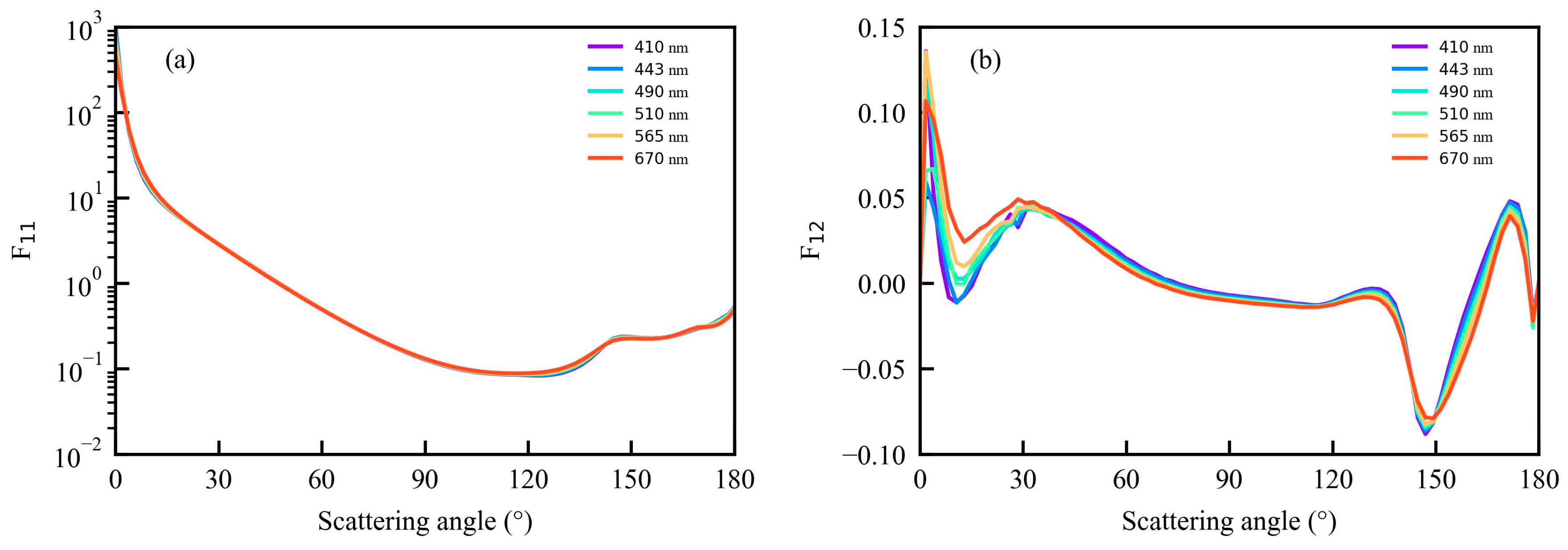
2.2.2. Optical Model of Case 1 Water

The research object in this paper is open ocean waters and the lower oceanic layer consists of pure sea water, phytoplankton, and colored dissolved organic matter (CDOM). The scattering coefficient of pure sea water is calculated by the Morel’s model [39]. The absorption coefficient of pure sea water is taken from Pope and Fry (i.e., 380~730 nm) [40]. The absorption and scattering coefficients of phytoplankton are computed using the Chla concentration [41,42]:
a p ( λ , [ Chla ] ) = A P ( λ ) × [ Chla ] E P ( λ )
b p ( λ , [ Chla ] ) = 0.30 × ( 550 λ ) × [ Chla ] 0.62
where a p ( λ , [ Chla ] ) and b p ( λ , [ Chla ] ) are the absorption and scattering coefficients of phytoplankton at wavelength λ (in nm) for a given Chla concentration [ Chla ] (in mg/m3), respectively. A P ( λ ) and E P ( λ ) are wavelength-dependent constant coefficients (i.e., the wavelength range is 400~700 nm) [41].
The CDOM is a purely absorbing particle, and its absorption coefficient is calculated as follows [43,44,45]:
a y ( λ , [ Chla ] ) = a y ( 440 , [ Chla ] ) × exp ( 0.014 × ( λ 440 ) ) ,
a y ( 440 , [ Chla ] ) = p 2 × a p ( 440 , [ Chla ] ) ,
p 2 = 0.3 + 5.7 × R 2 × a p ( 440 , [ Chla ] ) 0.02 + a p ( 440 , [ Chla ] ) .
where R 2 is a random number ranging from 0 to 1, and we use 0.5 in this study [44].
The backscattering ratio is defined as B b p = b b p / b p , where b b p is the backward scattering coefficient. The backscattering ratio of phytoplankton B b p ( [ Chla ] ) is spectrally independent [46]:
B b p ( [ Chla ] ) = 0.002 + 0.01 ( 0.5 0.25 log 10 [ Chla ] )
The size distribution of the phytoplankton-like particles is often assumed to follow the Junge power law [47]. In this paper, the Fournier–Forand (FF) phase function with Voss and Fry (VF) reduced Mueller matrix, which is chosen for the underwater particles. The VF reduced Mueller matrix provides the normalized light scattering polarization matrix derived from real measurements [48,49]. The FF phase function is an approximate analytic form used to describe particles with a Junge particle size distribution [50,51], and it is in good agreement with the measured Petzold phase function [52]. The FF phase function is determined as follows:
F F F ( Θ ) = 1 4 π ( 1 δ ) 2 δ v { v ( 1 δ ) ( 1 δ v ) + [ δ ( 1 δ v ) v ( 1 δ ) sin 2 ( Θ / 2 ) ] } + 1 δ 180 v 16 π ( δ 180 1 ) δ 180 v ( 3 cos 2 ( Θ ) 1 )
where:
v = 3 μ 2 ,   δ = 4 3 ( n 1 ) 2 sin 2 ( Θ / 2 )
Here, Θ is the scattering angle, δ 180 is the value of δ at Θ = 180 ° , μ is the slope parameter of the Junge distribution, and n is the real part of the refractive index of the particles.
The backscattering ratio can be obtained using Equation (5) [52]:
B bp FF = 1 1 δ 90 v + 1 0.5 ( 1 δ 90 v ) ( 1 δ 90 ) δ 90 v
where δ 90 is the value of δ at Θ = 90 ° . Further, a linear relationship between μ and n is proposed [52], namely:
n = 1.01 + 0.1542 ( μ 3 )
According to Equation (4), the value of B b p ( [ Chla ] ) for a given Chla concentration can be calculated. By performing best fits with a look-up table generated by Equations (6)–(8), the values of μ and n are obtained, which are the two model parameters of the FF phase function [53].
The bulk scattering matrix of open ocean water F B u l k can be written as:
F B u l k ( λ , Θ ) = b w ( λ ) F w ( Θ ) + b p ( λ ) F p ( Θ ) b w ( λ ) + b p ( λ )
where b w ( λ ) is the scattering coefficient of pure sea water. F w ( Θ ) represents the scattering matrix of pure sea water and is obtained through Rayleigh scattering. F p represents the scattering matrix of phytoplankton.

2.3. The Concept of Parallel Polarization Radiance

The vector radiation field of the coupled AOS can be expressed by the Stokes vector, as follows:
S = [ I Q U V ] = [ < E x 2 ( t ) > + < E y 2 ( t ) > < E x 2 ( t ) > < E y 2 ( t ) > < 2 E x ( t ) E y ( t ) cos δ > < 2 E x ( t ) E y ( t ) sin δ > ]
where I is the total intensity of the light beam, Q is the intensity difference between the polarized components of the electromagnetic wave parallel and perpendicular to the reference plane. U indicates the intensity difference between the polarized components in the planes 45° and −45° to the reference plane. V is the circularly polarized component, which is negligible for most cases of light scattered by the sea surface and atmosphere [54,55]. E x ( t ) and E y ( t ) are components of the electric vector in the local-view meridian plane (determined by a scatted beam in the view direction of the sensor and normal local surface) and in the plane perpendicular to the meridian plane, respectively. Moreover, δ is the phase difference between E x ( t ) and E y ( t ) , and the notation < > represents the time average. The PPR and VPR (vertical polarization radiance) are defined as follows [14]:
P P R = I + Q V P R = I Q
Based on the OSOAA and the input parameters of the model described in Section 2.2, we set a black ocean (i.e., light fully absorbed by the ocean) to simulate the reflectance of the I, PPR, and VPR just above the sea surface (0+) at 443 nm. The reflectance is, thus, the sum contribution of both the reflectance reflected by scattered skylight at the air–sea surface and the reflectance reflected by direct sunlight at the air–sea surface. The reflectance for the PPR at 0+ is defined as:
ρ 0 + ,   p p r = π P P R 0 + E s cos θ s
where E s is the extra-terrestrial solar irradiance and the solar zenith angle θ s is set to 30°. The reflectance for the I or VPR can be obtained by replacing the PPR.
As shown in Figure 2, the smallest of the three reflectance is ρ 0 + ,   P P R , which can also be observed at other wavelengths. Therefore, selecting the PPR can reduce the sea surface effects [14]. Unlike the second and third Stokes vectors (Q, U), the PPR has a similar physical meaning to I and represents the intensity of the parallel polarization radiance, making PPR easier to apply in ocean remote sensing.

2.4. Definition of the Radiation Field at the TOA

The total reflectance for the I and PPR at the TOA are, respectively, represented as:
ρ t = π I t E s cos θ s ρ t , p p r = π P P R t E s cos θ s
where I t is the TOA total radiance from all the components of the AOS, including the atmosphere, ocean surface, and phytoplankton in the seawater. P P R t is the TOA total parallel polarization radiance.
The water-leaving signals for the I and PPR at the TOA are defined as:
ρ w = π I w E s cos θ s ρ w , p p r = π P P R w E s cos θ s
where I w is the water-leaving radiance contribution at the TOA. P P R w is the water-leaving parallel polarization radiance contribution at the TOA. I w is expressed in this article as:
I w = I t I t , b
where I t , b is the background radiance at the TOA, which equates to an AOS with the same atmosphere and sea surface, but with a black ocean. Similarly, P P R w is calculated using:
P P R w = P P R t P P R t , b
where P P R t , b is the background parallel polarization radiance at the TOA.

2.5. Back-Propagation Neural Network

The back-propagation neural network is a multi-layer feed-forward neural network that considers the backward error. The BPNN can use nonlinear units (neurons) to map input–output nonlinear features and is widely used in the estimation of water quality parameters [6]. The outstanding advantage of BPNN is that a unique transfer function is added to each neuron of the network, and the network weights are adjusted during each training process through the error backpropagation technique. The input layer, hidden layer, and output layer constitute the most basic BPNN structure, and each layer is connected by neurons.

3. Results and Discussion

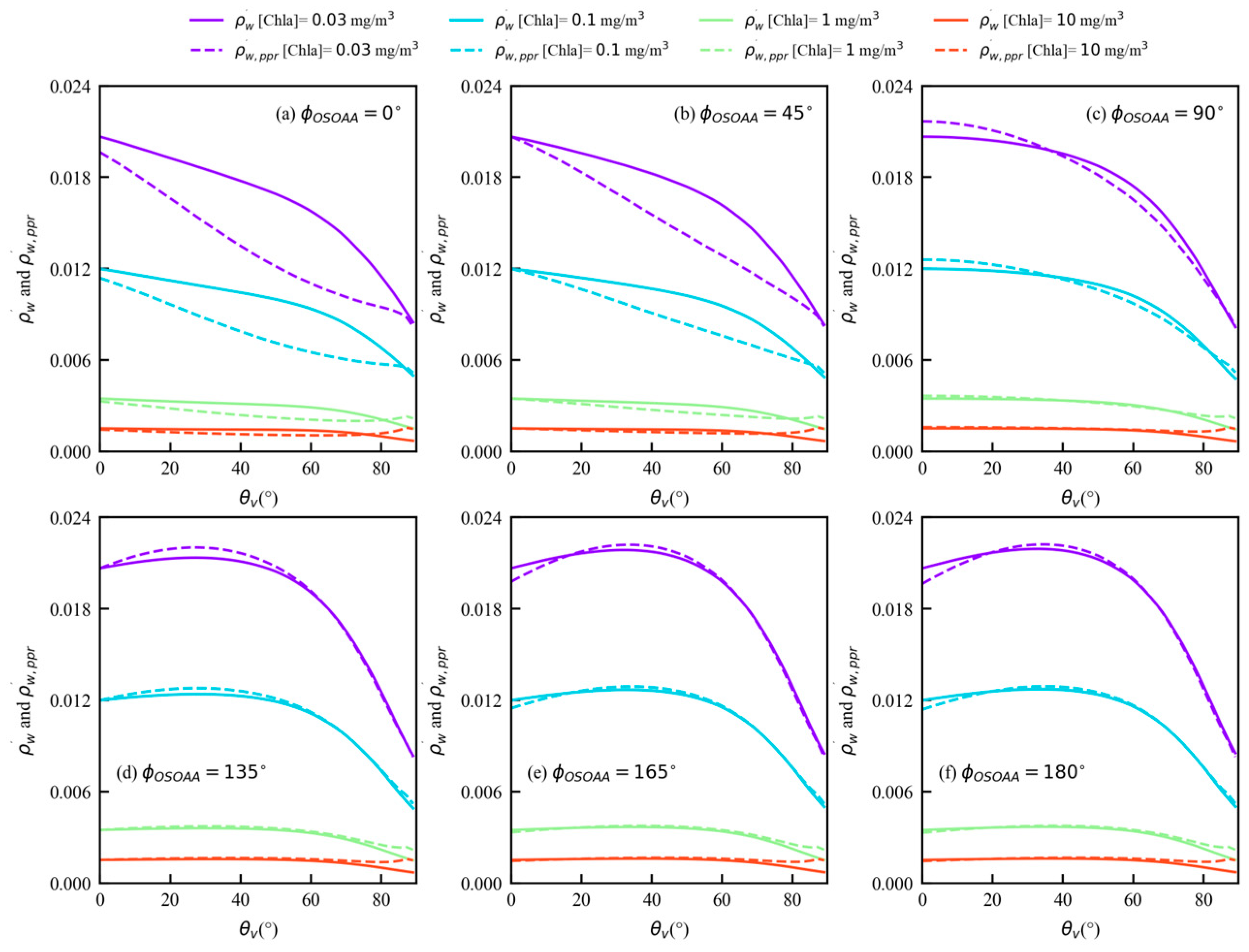
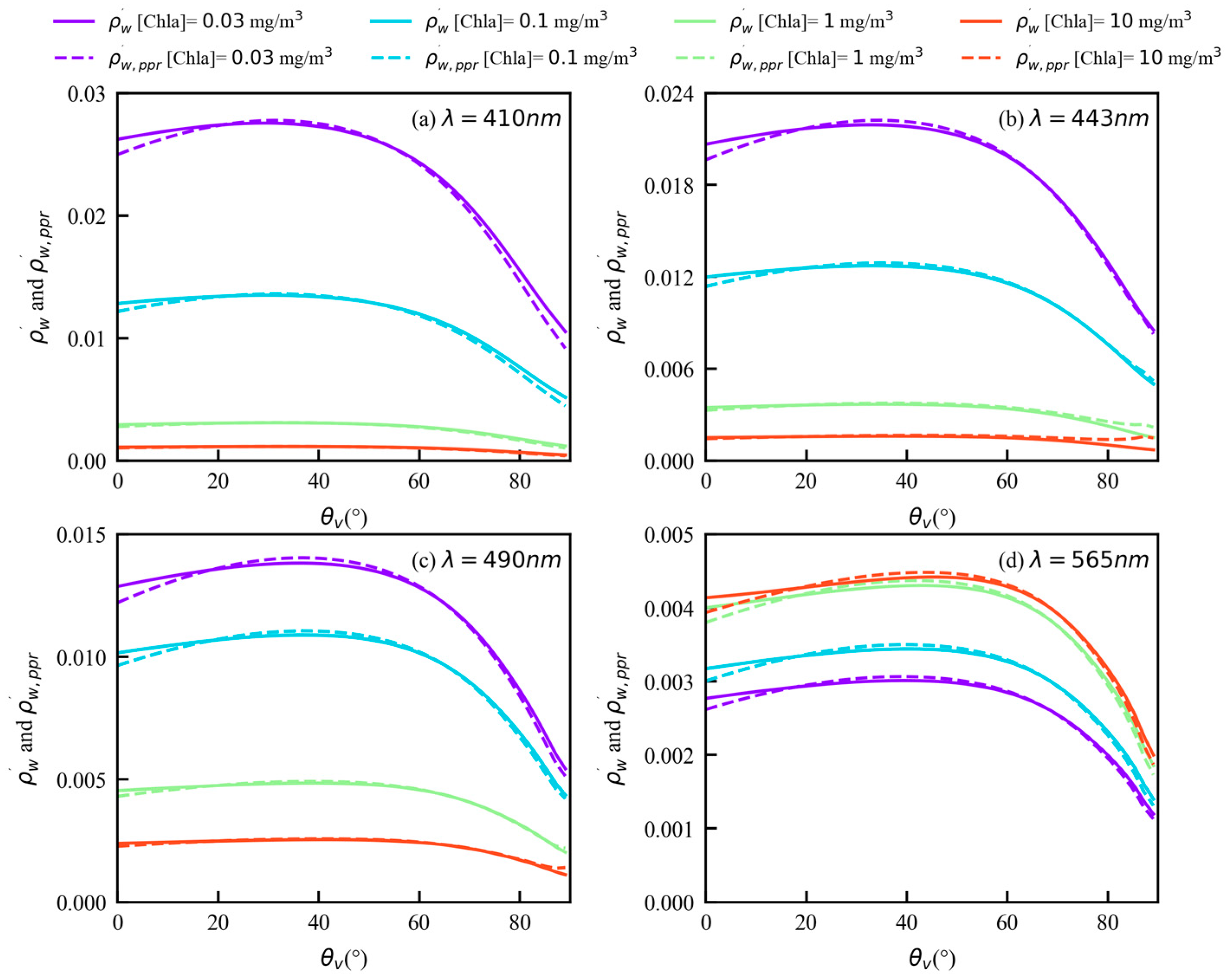
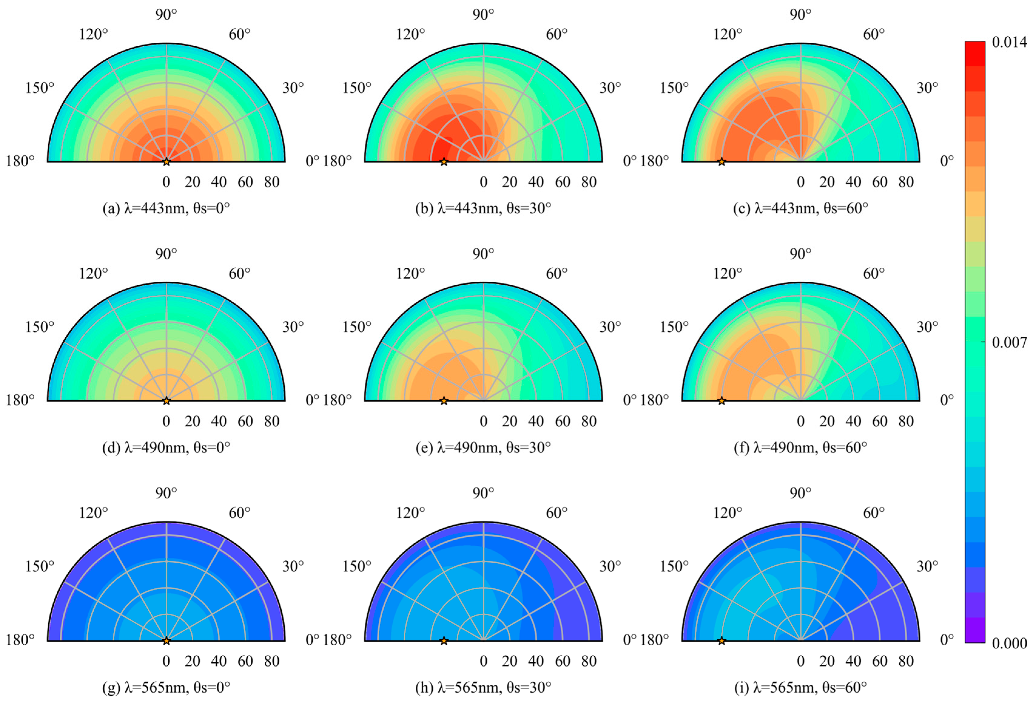
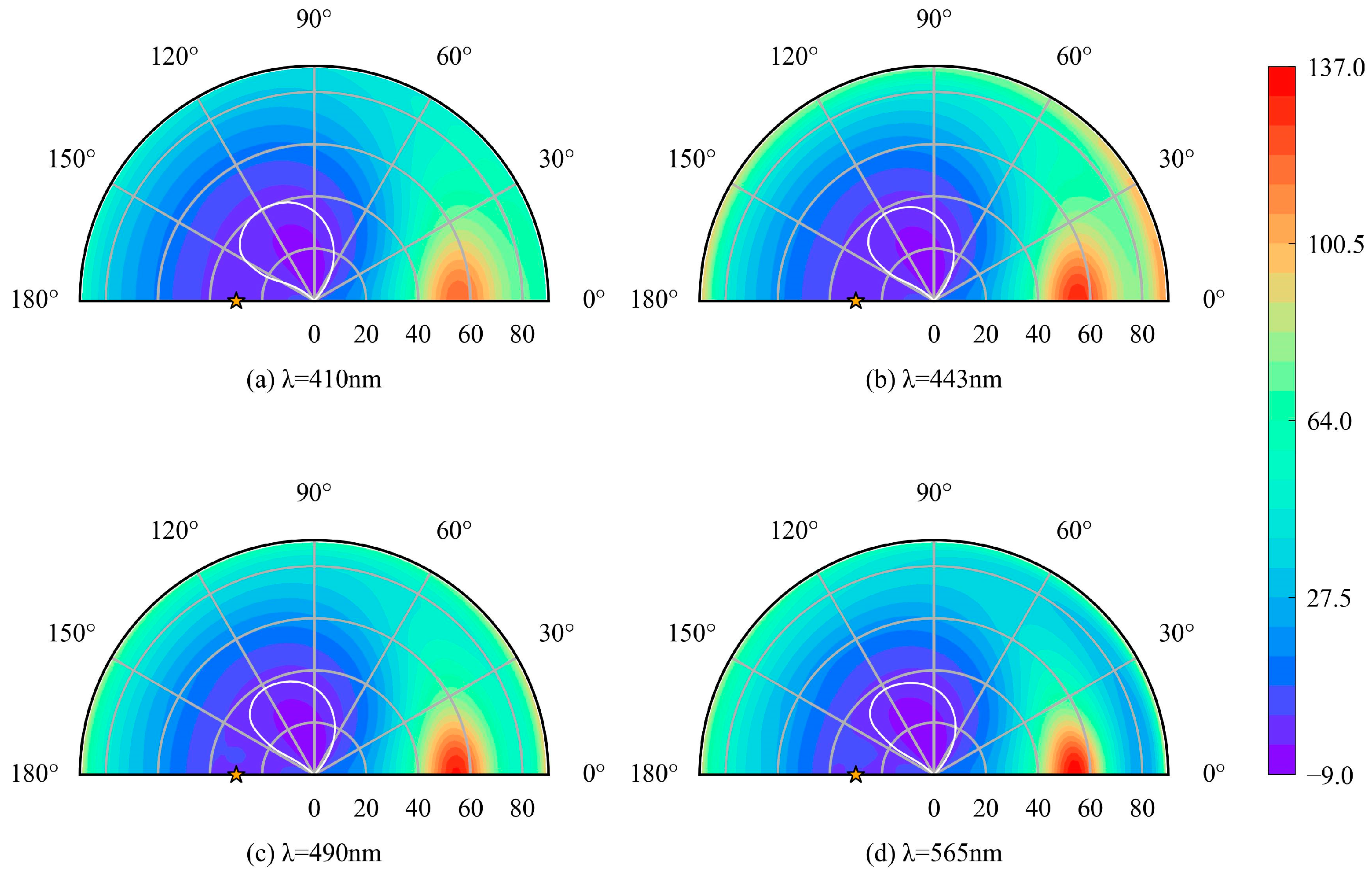
3.1. Angular Variation of TOA PPR Reflectance

Figure 3 displays the polar diagram of the angular variations of the reflectance for the I and PPR at 443 nm at the TOA. Figure 4 is the same as Figure 3, but for 565 nm. In these figures, the solar zenith angle θ s is 30° and the Chla concentration [ Chla ] is 0.1 mg/m3. The radial coordinate represents the viewing zenith angle θ v , and the angular coordinate represents the relative azimuth angle φ O S O A A . The azimuth angle of 180° corresponds to the backscattering half-plane (i.e., the sensor and the sun are in the same half-plane). The azimuth angle of 0° corresponds to the specular half-plane (i.e., the sensor and the sun are located in opposite half-planes), which contains sunglint. As shown in Figure 3a,b and Figure 4a,b, the angular distributions of the TOA reflectance ρ t , p p r and ρ t are similar, and the values for both are larger at a high zenith angle, this is because the total reflectance at the TOA is mainly affected by the atmospheric layer [56]. The longer atmospheric path length increases the effect of atmospheric scattering with the increase in the viewing zenith angle. The phase matrices of the atmosphere and ocean determine the exact location of the minimum total reflectance, which is usually near the nadir point [57]. The reflectance ρ t , p p r is significantly smaller than ρ t within relative azimuth angles φ O S O A A ranging from 0° to 60° and the viewing zenith angles θ v ranging from 30° to 75°. Similar result can also be obtained for a large viewing zenith angle θ v (e.g., 75°~90°).
Figure 3c,d and Figure 4c,d show the angular variation of ρ w is smaller, while the azimuth variation of ρ w , p p r is larger. The angular distributions for ρ w , p p r and ρ w are different for a region located in the range of φ O S O A A between 0° to 60°, where the values of ρ w are higher than that of ρ w , p p r . Figure 5 shows the maximum value of ρ w , p p r (0.0129) is bigger than that of ρ w (0.0127) at 443 nm when the Chla concentration is 0.1 mg/m3, and both maximum values occur in the backscattering direction but do not exactly align with the solar zenith angle. At different Chla concentrations, similar variations for ρ w , p p r and ρ w as function of the viewing zenith angle can be observed within the φ O S O A A of 90° to 180°. The water-leaving signal at the TOA is the smallest at a large viewing zenith angle due to the increase in atmospheric attenuation. For all azimuth angles, the water-leaving signals for I and PPR at 443 nm decrease with increasing Chla concentration, and their variation curves with respect to the viewing zenith angle are more uniform for a high Chla concentration.
Figure 6 shows that the water-leaving signals for I and PPR exhibit similar angular variations and magnitudes in the backscattering half-plane. Figure 7 shows the polar diagram of the water-leaving signal for the PPR at the TOA at 443 nm, 490 nm, and 565 nm, for different solar zenith angles (0°, 30°, and 60°). Notably, at a solar zenith angle of 0°, the angular distribution of the water-leaving signal ρ w , p p r is symmetrical. As the solar zenith angle increases, the symmetry of ρ w , p p r is disrupted, and the maximum value of ρ w , p p r changes with the solar zenith angle, moving towards the backscattering direction. The observation geometry can significantly affect the angular variation of ρ w , p p r , especially at solar zenith angles of 30° and 60°.

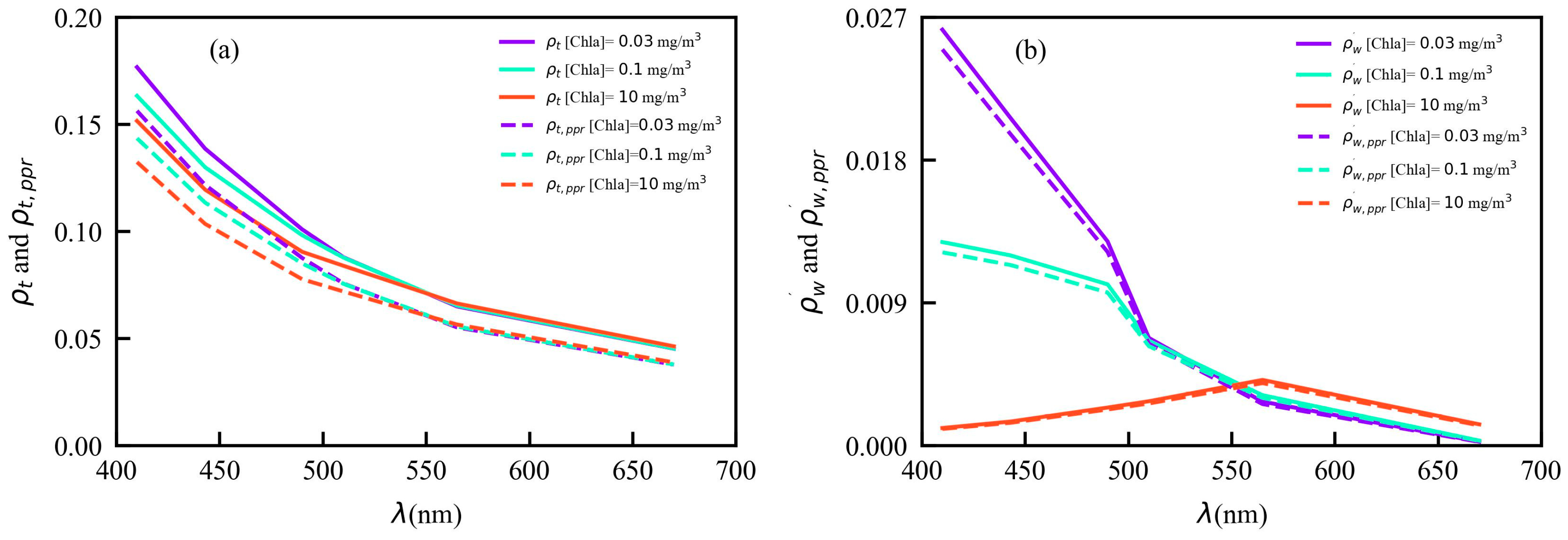
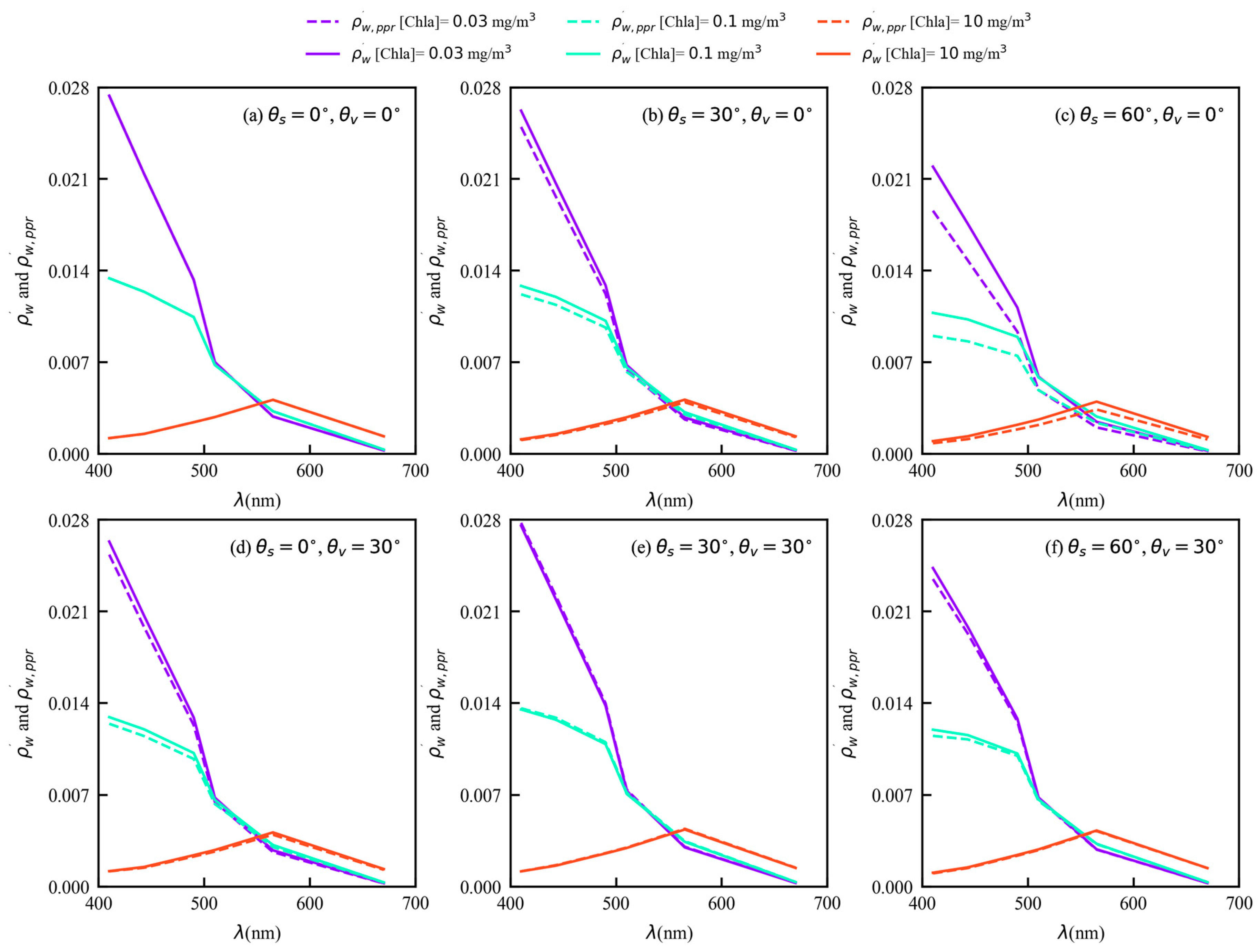
3.2. Spectral Variation of TOA PPR Reflectance

Figure 8 shows spectral variation of TOA reflectance at the nadir point for different Chla concentrations. As shown in Figure 8a, the spectral variation of ρ t , p p r is similar to ρ t but with a lower value. The total reflectance at the TOA is smaller for longer wavelengths, owing to the decreasing molecular and aerosol scattering with increasing wavelength. This demonstrates that atmosphere scattering is the predominant contributor to the TOA total reflectance in visible bands.
Figure 8b shows the value of ρ w is slightly higher than that of ρ w , p p r . The water-leaving signal ρ w decreases with the increase in the Chla concentration at 410 nm and 443 nm, this is due to the fact that chlorophyll has a strong ability to absorb blue light. When the Chla concentration changes from 0.03 to 10 mg/m3, ρ w at 410 nm decreases by 0.025. There is an inflection wavelength around 550 nm, where ρ w is nearly independent of the Chla concentration. At 565 nm and 670 nm, the reflectance ρ w increases as the Chla concentration increases, due to a stronger backscattering and a weaker absorption effect. The above results are the theoretical basis of the band ratio method for the Chla concentration retrieval algorithm, and the water-leaving signal for the PPR has similar spectral characteristics. Furthermore, the spectral variations and magnitudes of the reflectance ρ w and ρ w , p p r are similar under different observation geometries (Figure 9).
Figure 8b shows the largest water-leaving signal for the PPR is found in the blue wavelength for [Chla] = 0.03 mg/m3 and [Chla] = 0.1 mg/m3. The reflectance ρ w , p p r decreases as the wavelength increases to 670 nm. For [Chla] = 10 mg/m3, the maximum ρ w , p p r occurs at 565 nm, because of the combined effect of the spectral variations of the total absorption and scattering coefficients [57]. On both sides of the maximum, as the wavelength approaches 410 nm and 670 nm, the value of ρ w , p p r decreases. In particular, the water-leaving signal for the PPR has a minimum at 670 nm. This is due to the higher absorption coefficient of seawater and the lower scattering coefficient of phytoplankton.

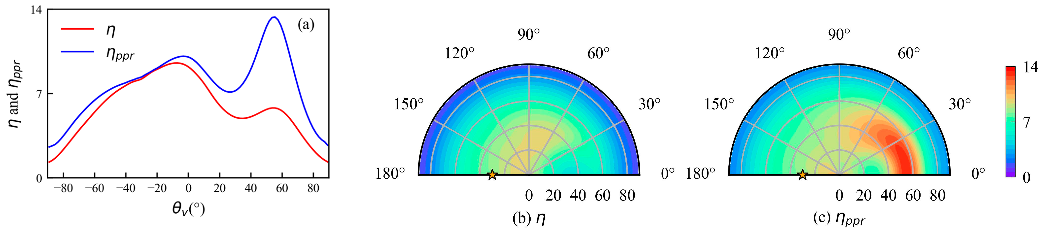
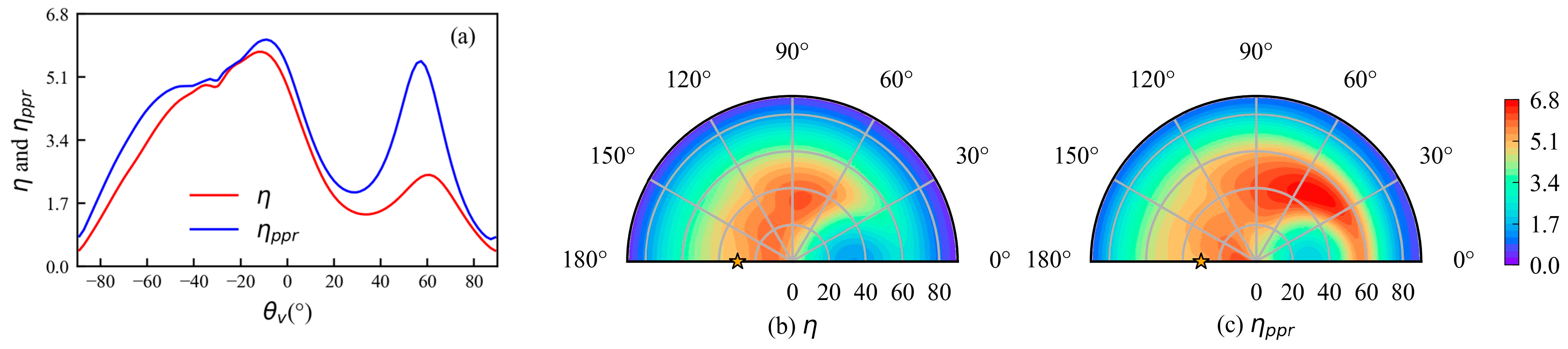
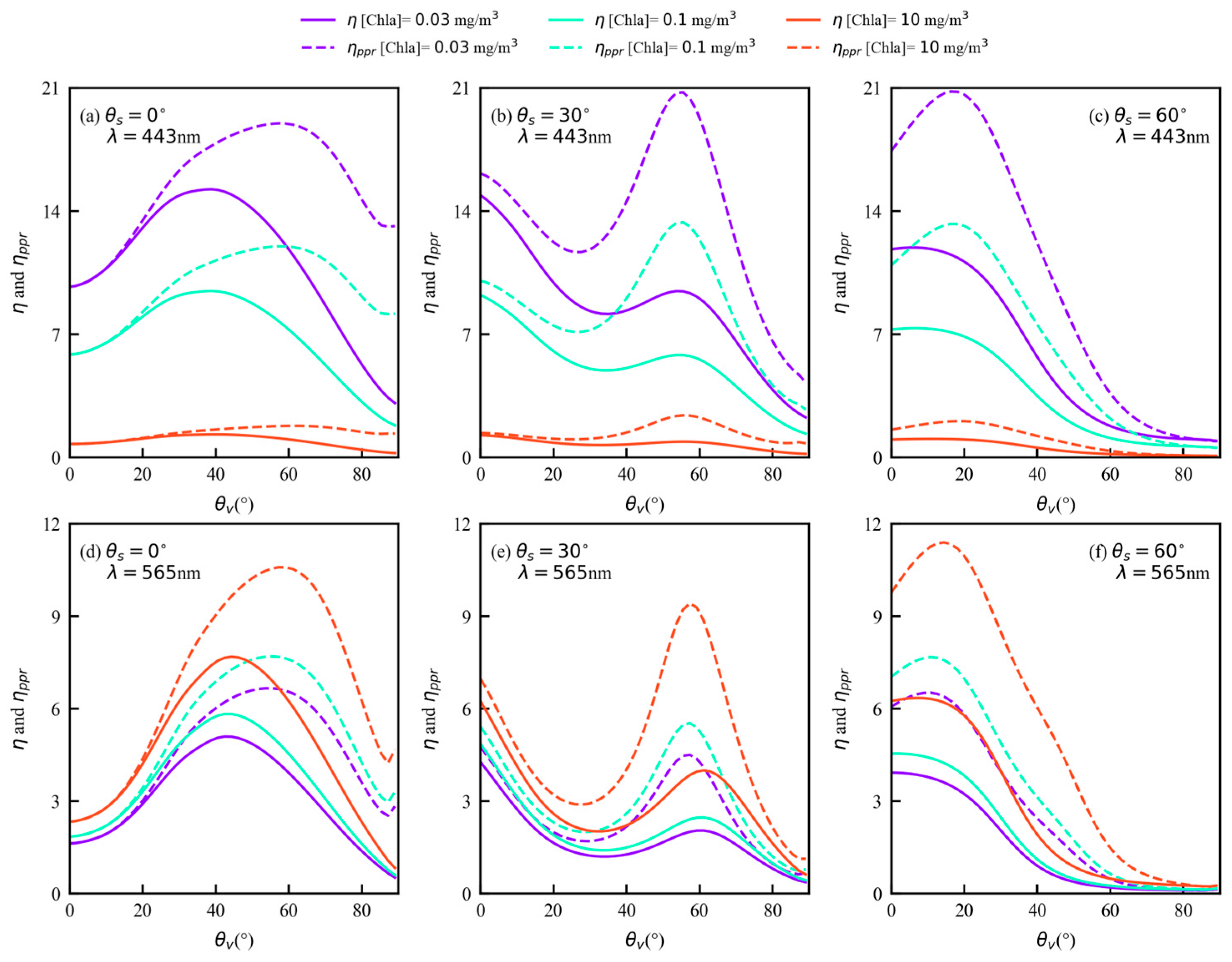
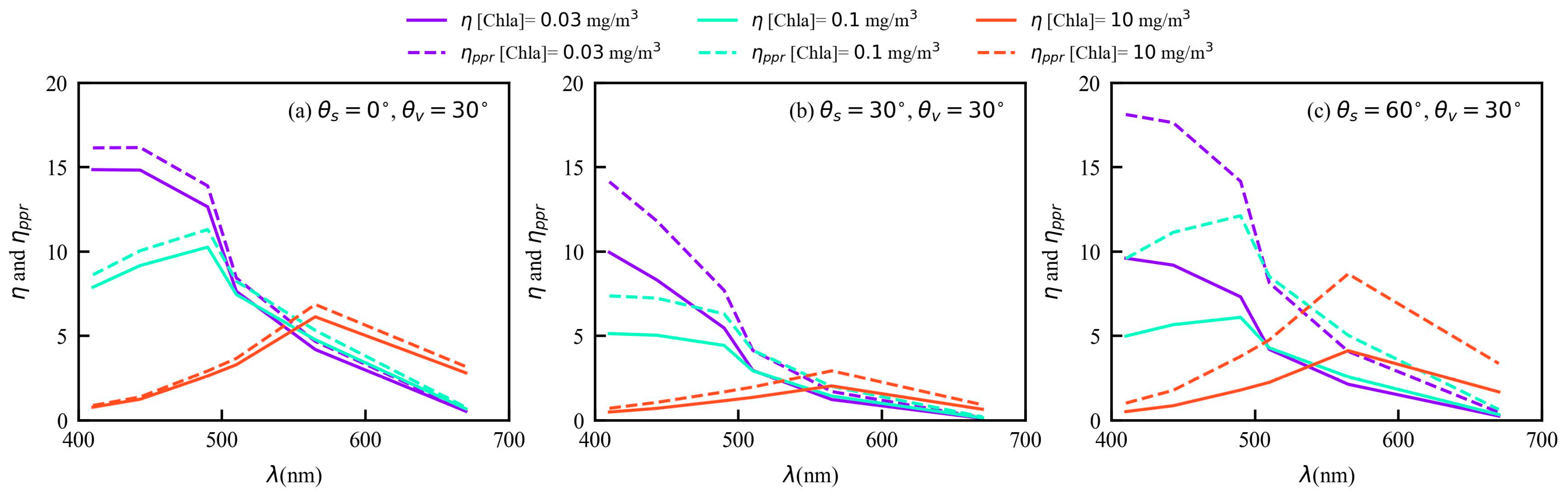
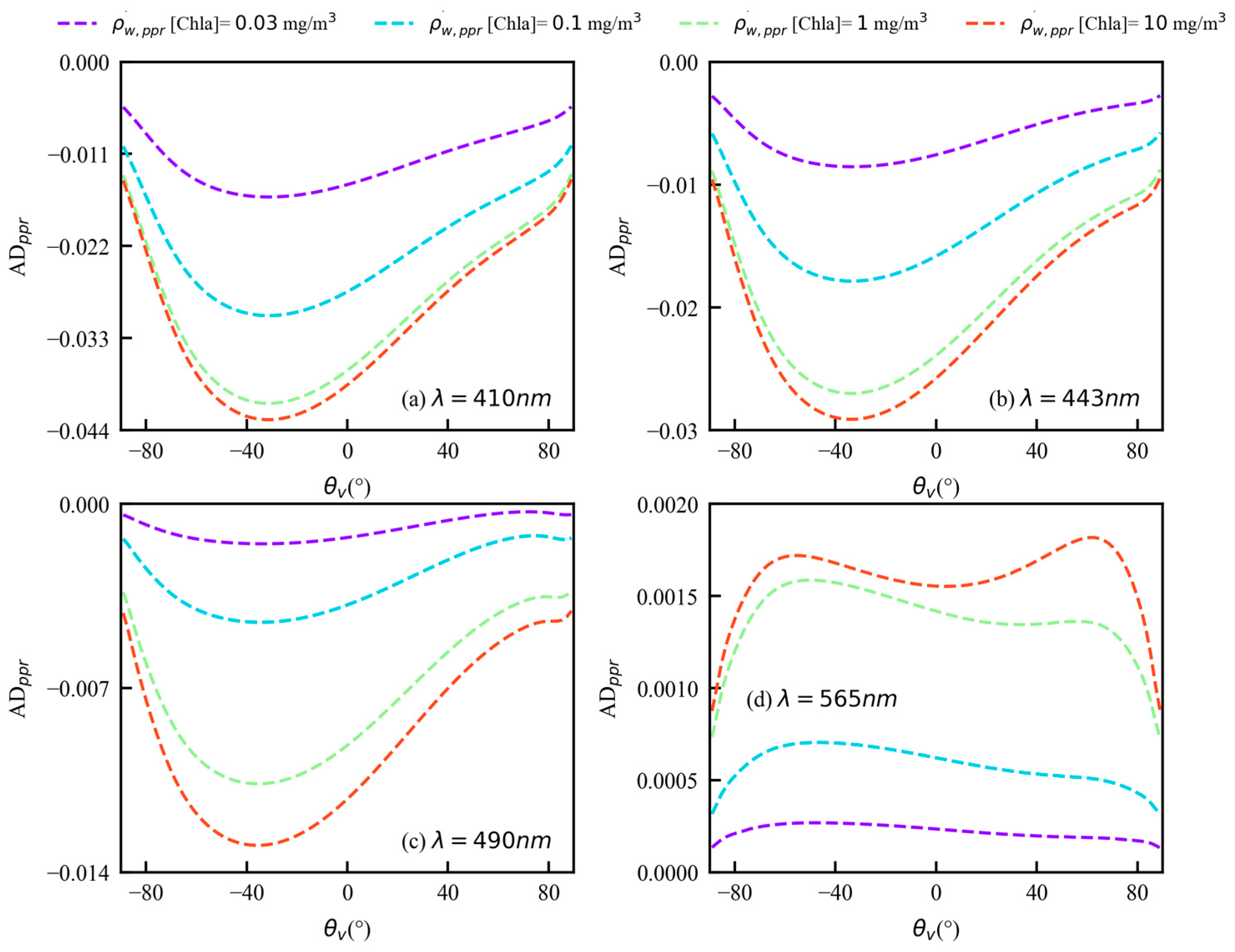
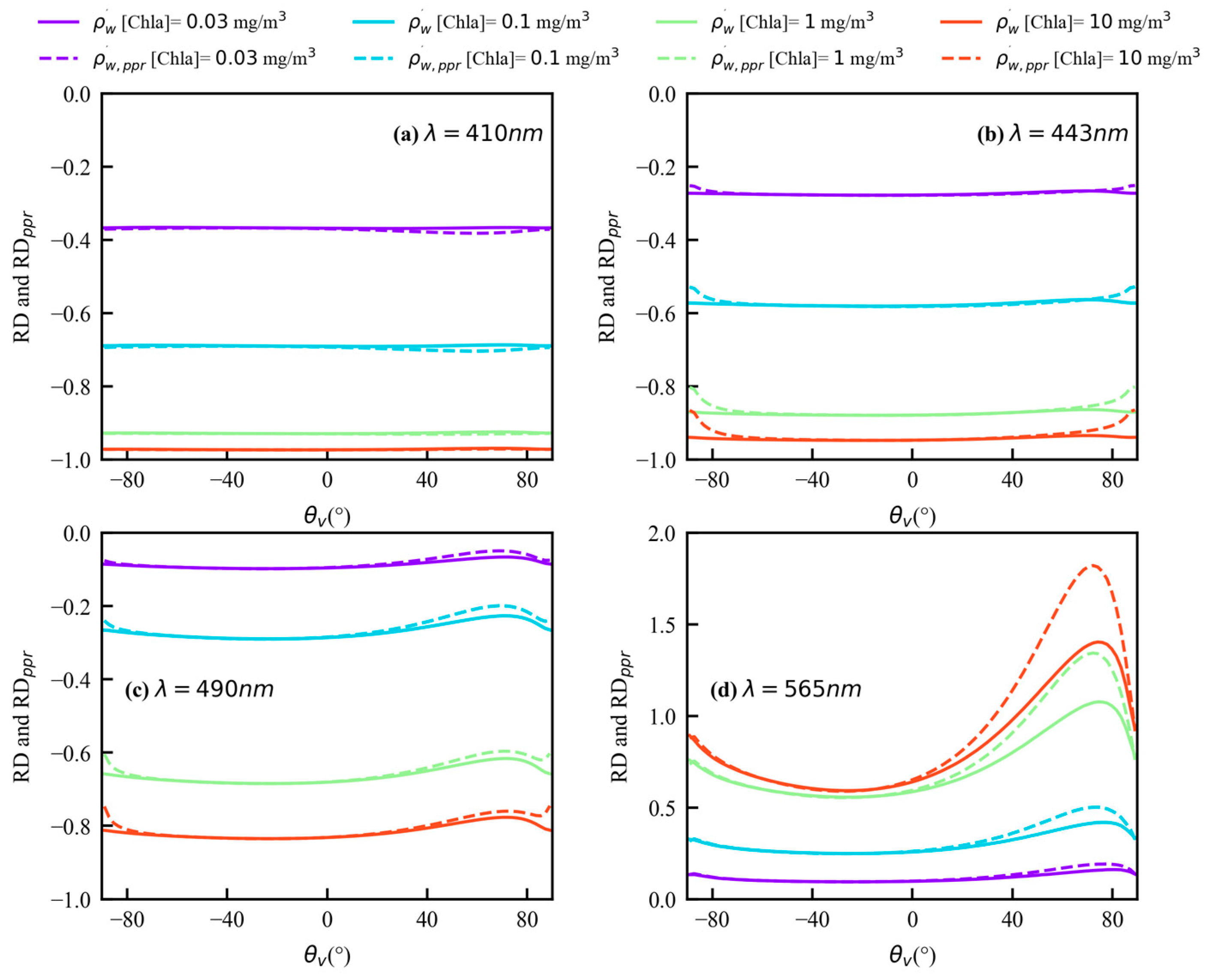
3.3. Enhancement of Contributions of the Water-Leaving Signals by PPR

The relative contributions of the water-leaving signals for the I and PPR at the TOA are estimated in the following way:
η = 100 ρ w / ρ t η p p r = 100 ρ w , p p r / ρ t , p p r
The variations of η and η p p r are examined at 443 nm in the principal plane (Figure 10a). Figure 10a shows the value of η p p r is higher than η in the principal plane. The maximum value of η in the two half-planes is around 9.5%, which is consistent with previous research findings [57,58,59]. For the observation geometry of the sunglint, the value of η is minimal due to the pronounced influence of sunglint. The roughness of the sea surface induced by the wind enables the observation of the sunlight reflection effect within a range of ±20° from the specular direction ( θ v = + 30 ° ) [9]. However, the value of η p p r is much higher compared to that of η in this particular geometry. For example, η p p r is around 13.3% compared with 5.8% for η at the viewing zenith angle of 54°. Note that η p p r is mostly higher than η regardless of the variations in the viewing zenith and azimuth angle outside the principal plane (Figure 10b,c). Therefore, the PPR can enhance the relative contribution of the water-leaving signal, especially in the sunglint observation geometry (Figure 10 and Figure 11).
Figure 12 shows the comparisons of the TOA relative contributions of the water-leaving signals for the I and PPR at different solar zenith angles and Chla contributions. Obviously, the PPR can enhance the relative contribution of the water-leaving signal except for the observation geometry (with a sun zenith angle of 0° and a viewing zenith angle of less than 20°), where the PPR and I exhibit similar detection capabilities for the ocean color signal.
Figure 13 shows the spectral variations of η and η p p r at different solar zenith angles and Chla concentrations. The relative contribution of the water-leaving signal on the PPR is greater than that for the I at all wavelengths. In addition, the relative contributions of the PPR and I are noticeable between 410 nm and 565 nm for different Chla concentrations. Note that the change trend in the relative contribution η is consistent with the results by Zhai et al. [57] and Ottaviani et al. [60], where the result by Ottaviani et al. was simulated using field measurements from IOPs in open oceans.
We calculate the relative deviation of the relative contributions for the I and PPR at the TOA as:
χ = ( η p p r η η ) × 100 %
The PPR can significantly enhance the ocean color signals in most observation geometries, with the maximum enhancement (136.5%) observed in the sunglint observation geometry at 565 nm (Figure 14). The benefit of the PPR is attributed to the compensatory effect of Q and the total radiance [14,61]. As the viewing zenith angle increases, both the radiance and Q at the TOA increase, and the negative values of Q can partially offset the increase in radiance (Figure 3a,b). Moreover, the polarization reflectance at the TOA is insensitive to the Chla concentration in open ocean waters [62,63]. As shown in Figure 3c,d, the PPR does not substantially reduce the TOA water-leaving signal. Thus, the water-leaving relative contribution on the PPR increases.

3.4. Sensitivity of PPR Reflectance to Chla in Open Oceans

The sensitivity of the water-leaving signal for the PPR to the Chla in open oceans is investigated by analyzing the variations in ρ w , p p r with different Chla concentrations. To assess these variations, the absolute difference ( A D p p r ) and relative difference ( R D p p r ) between the reflectance ρ w , p p r calculated at a given Chla concentration and the reflectance ρ w , p p r calculated at a reference concentration are defined by:
A D p p r = Δ ρ w , p p r ( Chla , Chla ref ) = ρ w , p p r ( Chla ) ρ w , p p r ( Chla ref ) R D p p r = A D p p r / ρ w , p p r ( Chla ref )
where ref stands for the reference Chla concentration with a value of 0.01 mg/m3. The A D and R D for I can be obtained by replacing the reflectance ρ w , p p r with the reflectance ρ w .
Figure 15 shows the variations of A D p p r as a function of the viewing zenith angle in the principal plane at different wavelengths and Chla concentrations. Negative values of θ v are related to the backscattering half-plane and positive values are related to the specular half-plane. The A D p p r value at 565 nm is positive and increases with the increase in the Chla concentration, meaning that the reflectance ρ w , p p r also increases at 565 nm. On the other hand, the A D p p r values at 410 nm, 443 nm, and 490 nm are negative, indicating that as the Chla concentration increases, and the water-leaving signal for the PPR decreases. The absolute A D p p r at 443 nm ranges from 0.0027 to 0.0291, and its maximum appears at a viewing zenith angle of around −30°. The reflectance ρ w , p p r of these four wavelengths is linearly related to the Chla concentration. Similar results can also be observed in Figure 6.
Figure 16 shows the variation of R D p p r and R D , as a function of the viewing zenith angle in the principal plane at different wavelengths and Chla concentrations. The angular variations of R D p p r and R D are similar, and the absolute values of R D p p r are larger than R D in the majority of the observation geometries. For example, the small viewing zenith angle is around 0° for 410 nm, 443 nm, and 490 nm. The large viewing zenith angle is around 70° for 565 nm. This means that the sensitivity of the PPR to the Chla concentration is sufficient.

3.5. Chla Inversion Algorithm Based on BPNN

The datasets required for the neural network are obtained using OSOAA simulation; 90% of the synthetic datasets were randomly selected for model training, and the remaining 10% of the datasets were used for testing. We chose the K-fold cross-validation to randomly divide the training datasets into K groups. Among them, K-1 groups are used for model fitting, and the remaining group is used for model testing. This process should be repeated K times [64]. In this article, K is set to 10. By performing 10-fold cross-validation, inaccuracies in the model evaluation due to accidental segmentation of the dataset can be avoided.
The Chla concentrations were generated logarithmically with a range of 0.005~1.5 mg/m3, inducing an increased proportion of lower Chla concentrations, which makes the simulations more consistent with the realistic open ocean. Adding 5% Gaussian noise to the simulated reflectance corresponds with the performance of the actual instrument.

3.5.1. Architecture of the BPNN Algorithm

This study constructed a 3-layer BPNN model, with an input layer, a hidden layer, and an output layer. To investigate the effects of the ρ w , ρ w , p p r and PCF strategy on the retrieval of the Chla concentration, three different configurations of the input layer were examined. In the first configuration, the input layer consists of the water-leaving signal for the I at a nadir point obtained for four wavelengths, namely 410 nm, 443 nm, 490 nm, 565 nm. This case is referred to as case I. The second configuration is similar to the first configuration, but the reflectance ρ w is replaced with the reflectance ρ w , p p r . Such a configuration is referred to as case PPR. The input layers in case I and case PPR consist of four neurons, because four wavelengths are used.
In the third configuration, the input layer at 410 nm selects the water-leaving signal for the PPR at the nadir point, and the input layers at 443 nm, 490 nm, and 565 nm consist of the reflectance obtained for 17 scattering angles, respectively, namely 102°, 106°, 111°, 116°, 122°, 128°, 135°, 143°, 145°, 148°, 150°, 152°, 155°, 156°, 159°, 160°, and 161°. Note that the scattering angle of 150° corresponds to the observation at the nadir point. However, the input layer composition for the three wavelengths is different. Specifically, among all observation directions, the input layer at 490 nm selects the water-leaving signal for the PPR and the input layer at 565 nm uses the water-leaving signal for the I. For the input layer at 443 nm, select the water-leaving signal for the PPR at the nadir point and choose the water-leaving signal for the I for the remaining observation directions. The third configuration described above is intended to be consistent with the PCF strategy and, therefore, is referred to as the case PCF. In the case PCF, the input layer contains 52 neurons.
The output layer only contains one neuron, representing the Chla concentration. For each neural network model, the optimal number of hidden layer neurons is determined through experiments [26].

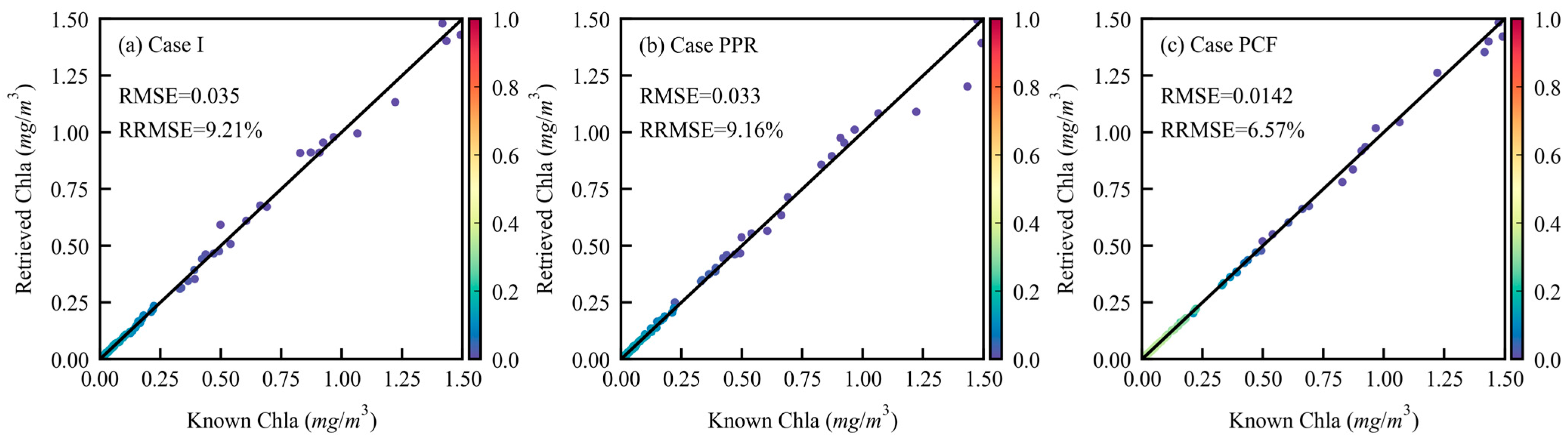
3.5.2. Chla Inversion Results

The root mean square error (RMSE) and the relative root mean square error (RRMSE) were used to evaluate the performance of the neural networks in three cases. The RMSE and RRMSE are defined as:
R M S E = 1 n i = 1 n ( Chla known i Chla retrieved i ) 2 R R M S E = 1 n i = 1 n ( Chla known i Chla retrieved i Chla known i ) 2
where n is the number of the validation datasets; Chla known i is the known Chla concentration used for the simulation, and Chla retrieved i is the Chla concentration retrieved from the BPNN. We used the following formula to evaluate the differences between case I and the other cases (PPR and PCF):
Δ R M S E x = R M S E x R R M S E I
where subscript x represents case PPR or PCF, and subscript I represents case I.
The inversion results from three BPNN models were evaluated using the validation datasets (see Table 2). Figure 17 shows the comparison between the retrieved values and the known values for the three cases. The models with three different configurations have good performance, and the coefficients of determination are close to 1. Similar results were also observed for the training datasets. Figure 17a,b indicates that the performance of the model of the Chla retrieval is better for the water-leaving signal of the PPR compared with the water-leaving signal of the I, with an RMSE value of 0.033 and an RRMSE value of 9.16%. The RMSE of the Chla retrieval for case PPR is approximately 0.002 lower than that of case I. This means that the PPR performs better in the retrieval of Chla in open oceans compared to the I.
Compared with case I and PPR, case PCF not only has the lowest RMSE (0.014) and RRMSE (6.57%), but also the slope in the linear model is the closest to 1 (Figure 17c). The RMSE decreases by around 0.021 when case PCF is considered. Therefore, the PCF strategy considering multi-directional and polarimetric detection significantly enhances the accuracy of the Chla retrieval.

4. Conclusions

In this paper, the impacts of both the PPR at the TOA and the PCF strategy on the retrieval of Chla concentrations in open oceans has been investigated, based on the OSOAA radiative transfer model. The spectrum ranges from 410 nm to 670 nm, covering the bands sensitive to Chla, as well as the bands set by the PCF.
First, the angular and spectral variations of the TOA reflectance for the I and PPR were examined. The results revealed that the values on the angular pattern of total reflectance for the PPR are smaller than that for the I. The water-leaving signals for the I and PPR at the TOA have the same magnitude in most observation geometries, and the maximum water-leaving signal for the PPR is higher. Therefore, the relative contribution of the water-leaving signal on the PPR is enhanced. Moreover, the water-leaving signal for the PPR exhibits significant directional and spectral variations relative to the observation geometries and Chla concentrations. The maximum value of ρ w , p p r appears in the backscattering direction at 410 nm. When the Chla concentration is 0.03 and 0.1 mg/m3, the largest relative contribution by the PPR is found at 410 nm. With an increase in the Chla concentration to 10 mg/m3, the maximum contribution is observed at 565 nm. Note that the water-leaving signal for the PPR is more sensitive to Chla concentration variations than that of I in the majority of observation geometries, especially at 565 nm and a high Chla concentration (10 mg/m3). Finally, the influence of the polarization and multi-directionality of the reflectance at the TOA on the retrieval of the Chla concentrations (ranging from 0.1 to 1.5 mg/m3) was studied based on the BPNN. The results showed that the water-leaving signal for the PPR slightly improved the accuracy of the Chla retrieval compared to that of I. Thus, the PPR can more comprehensively characterize the information on marine components. In the three cases, the PCF strategy performed best, with an RMSE of 0.014 and an RRMSE of 6.57%. This indicates that the polarization and directionality of the reflectance can improve the inversion of Chla in open oceans.
In conclusion, it is beneficial for ocean color remote sensing to take into account the directionality and polarization of the reflectance. The PPR can reduce sea surface effects and enhance the relative contribution of the water-leaving signal at the TOA. Our results indicate that the PCF data received from the Gaofen-5B satellite has encouraging potential for ocean color remote sensing in open oceans.

Author Contributions

Conceptualization, Y.W. (Yichen Wei) and X.S.; methodology, Y.W. (Yichen Wei), H.Y. and Y.W. (Yuxuan Wang); validation, Y.W. (Yichen Wei); software, Y.W. (Yichen Wei), Y.W. (Yuxuan Wang) and Y.L.; writing—original draft preparation, Y.W (Yichen Wei); writing—review and editing, X.S., X.L., H.H., R.T. and J.H.; visualization, Y.W. (Yichen Wei) and Y.W. (Yuyao Wang); supervision, X.S.; project administration, X.S. and X.L.; funding acquisition, X.S. All authors have read and agreed to the published version of the manuscript.

Funding

This work was supported by the Aerospace Science and Technology Innovation Application Research Project (E23Y0H555S1), the Aviation Science and Technology Innovation Application Research Project (62502510201), the China High-Resolution Earth Observation System (CHEOS)(30-Y20A010-9007-17/18), and the China Center for Resource Satellite Data and Applications Project (E13Y0J31601).

Data Availability Statement

Data are contained within the article.

Acknowledgments

The authors thank the development team on the payload for the Gaofen-5B satellite at Anhui Institute of Optics and Fine Mechanics, Chinese Academy of Sciences (CAS), Hefei, China. In addition, we would like to thank the Centre National d’Etudes Spatiales (CNES-France) for the maintenance and the online distribution of the OSOAA radiative transfer model (https://github.com/CNES/RadiativeTransferCode-OSOAA, accessed on 17 August 2022). We are grateful for the constructive comments provided by the editor and the anonymous reviewers on this paper.

Conflicts of Interest

The authors declare no conflict of interest.

References

  1. Boyce, D.G.; Lewis, M.R.; Worm, B. Global phytoplankton decline over the past century. Nature 2010, 466, 591–596. [Google Scholar] [CrossRef] [PubMed]
  2. Falkowski, P.G.; Katz, M.E.; Knoll, A.H.; Quigg, A.; Raven, J.A.; Schofield, O.; Taylor, F.J. The evolution of modern eukaryotic phytoplankton. Science 2004, 305, 354–360. [Google Scholar] [CrossRef]
  3. Marzano, F.S.; Iacobelli, M.; Orlandi, M.; Cimini, D. Coastal Water Remote Sensing from Sentinel-2 Satellite Data Using Physical, Statistical, and Neural Network Retrieval Approach. IEEE Trans. Geosci. Remote Sens. 2021, 59, 915–928. [Google Scholar] [CrossRef]
  4. IOCCG. Phytoplankton Functional Types from SPACE; Reports of the International Ocean Colour Coordinating Group; IOCCG: Dartmouth, NS, Canada, 2014; Volume 15, p. 153. [Google Scholar]
  5. Ibrahim, A.; Gilerson, A.; Chowdhary, J.; Ahmed, S. Retrieval of macro- and micro-physical properties of oceanic hydrosols from polarimetric observations. Remote Sens. Environ. 2016, 186, 548–566. [Google Scholar] [CrossRef]
  6. Xu, S.Q.; Li, S.J.; Tao, Z.; Song, K.S.; Wen, Z.D.; Li, Y.; Chen, F.F. Remote Sensing of Chlorophyll-a in Xinkai Lake Using Machine Learning and GF-6 WFV Images. Remote Sens. 2022, 14, 5136. [Google Scholar] [CrossRef]
  7. El-Habashi, A.; Bowles, J.; Foster, R.; Gray, D.; Chami, M. Polarized observations for advanced atmosphere-ocean algorithms using airborne multi-spectral hyper-angular polarimetric imager. J. Quant. Spectrosc. Radiat. Transf. 2021, 262, 107515. [Google Scholar] [CrossRef]
  8. Gao, M.; Zhai, P.W.; Franz, B.A.; Hu, Y.X.; Knobelspiesse, K.; Werdell, P.J.; Ibrahim, A.; Cairns, B.; Chase, A. Inversion of multiangular polarimetric measurements over open and coastal ocean waters: A joint retrieval algorithm for aerosol and water-leaving radiance properties. Atmos. Meas. Tech. 2019, 12, 3921–3941. [Google Scholar] [CrossRef]
  9. Chami, M.; Larnicol, M.; Minghelli, A.; Migeon, S. Influence of the Suspended Particulate Matter on the Satellite Radiance in the Sunglint Observation Geometry in Coastal Waters. Remote Sens. 2020, 12, 1445. [Google Scholar] [CrossRef]
  10. Gordon, H.R.; Wang, M. Retrieval of water-leaving radiance and aerosol optical thickness over the oceans with SeaWiFS: A preliminary algorithm. Appl. Opt. 1994, 33, 443–452. [Google Scholar] [CrossRef]
  11. Zhou, G.; Xu, W.; Niu, C.; Zhao, H. The polarization patterns of skylight reflected off wave water surface. Opt. Express 2013, 21, 32549–32565. [Google Scholar] [CrossRef]
  12. Fougnie, B.; Frouin, R.; Lecomte, P.; Deschamps, P.Y. Reduction of skylight reflection effects in the above-water measurement of diffuse marine reflectance. Appl. Opt. 1999, 38, 3844–3856. [Google Scholar] [CrossRef] [PubMed]
  13. Frouin, R.; Pouliquen, E.; Bréon, F.-M. Ocean color remote sensing using polarization properties of reflected sunlight. In Proceedings of the CNES, 6th International Symposium on Physical Measurements and Signatures in Remote Sensing, Val d’Isère, France, 17–22 January 1994; pp. 665–674. [Google Scholar]
  14. He, X.; Pan, D.; Bai, Y.; Wang, D.; Hao, Z. A new simple concept for ocean colour remote sensing using parallel polarisation radiance. Sci. Rep. 2014, 4, 3748. [Google Scholar] [CrossRef]
  15. Liu, J.; He, X.; Liu, J.; Bai, Y.; Wang, D.; Chen, T.; Wang, Y.; Zhu, F. Polarization-based enhancement of ocean color signal for estimating suspended particulate matter: Radiative transfer simulations and laboratory measurements. Opt. Express 2017, 25, A323–A337. [Google Scholar] [CrossRef] [PubMed]
  16. Harmel, T.; Chami, M. Influence of polarimetric satellite data measured in the visible region on aerosol detection and on the performance of atmospheric correction procedure over open ocean waters. Opt. Express 2011, 19, 20960–20983. [Google Scholar] [CrossRef] [PubMed]
  17. Chowdhary, J.; Cairns, B.; Waquet, F.; Knobelspiesse, K.; Ottaviani, M.; Redemann, J.; Travis, L.; Mishchenko, M. Sensitivity of multiangle, multispectral polarimetric remote sensing over open oceans to water-leaving radiance: Analyses of RSP data acquired during the MILAGRO campaign. Remote Sens. Environ. 2012, 118, 284–308. [Google Scholar] [CrossRef]
  18. Gao, M.; Zhai, P.W.; Franz, B.; Hu, Y.; Knobelspiesse, K.; Werdell, P.J.; Ibrahim, A.; Xu, F.; Cairns, B. Retrieval of aerosol properties and water-leaving reflectance from multi-angular polarimetric measurements over coastal waters. Opt. Express 2018, 26, 8968–8989. [Google Scholar] [CrossRef]
  19. Hansen, J.E.; Travis, L.D. Light-Scattering in Planetary Atmospheres. Space Sci. Rev. 1974, 16, 527–610. [Google Scholar] [CrossRef]
  20. Espinosa, W.R.; Martins, J.V.; Remer, L.A.; Dubovik, O.; Lapyonok, T.; Fuertes, D.; Puthukkudy, A.; Orozco, D.; Ziemba, L.; Thornhill, K.L.; et al. Retrievals of Aerosol Size Distribution, Spherical Fraction, and Complex Refractive Index from Airborne In Situ Angular Light Scattering and Absorption Measurements. J. Geophys. Res. Atmos. 2019, 124, 7997–8024. [Google Scholar] [CrossRef]
  21. Liu, J.; Hu, B.L.; He, X.Q.; Bai, Y.; Tian, L.Q.; Chen, T.Q.; Wang, Y.H.; Pan, D.L. Importance of the parallel polarization radiance for estimating inorganic particle concentrations in turbid waters based on radiative transfer simulations. Int. J. Remote Sens. 2020, 41, 4923–4946. [Google Scholar] [CrossRef]
  22. Liu, J.; Liu, J.; He, X.; Tian, L.; Bai, Y.; Chen, T.; Wang, Y.; Zhu, F.; Pan, D. Retrieval of marine inorganic particle concentrations in turbid waters using polarization signals. Int. J. Remote Sens. 2019, 41, 4901–4922. [Google Scholar] [CrossRef]
  23. Gilerson, A.; Zhou, J.; Oo, M.; Chowdhary, J.; Gross, B.M.; Moshary, F.; Ahmed, S. Retrieval of chlorophyll fluorescence from reflectance spectra through polarization discrimination: Modeling and experiments. Appl. Opt. 2006, 45, 5568–5581. [Google Scholar] [CrossRef]
  24. Ibrahim, A.; Gilerson, A.; Harmel, T.; Tonizzo, A.; Chowdhary, J.; Ahmed, S. The relationship between upwelling underwater polarization and attenuation/absorption ratio. Opt. Express 2012, 20, 25662–25680. [Google Scholar] [CrossRef] [PubMed]
  25. Freda, W.; Haule, K.; Sagan, S. On the role of the seawater absorption-to-attenuation ratio in the radiance polarization above the southern Baltic surface. Ocean Sci. 2019, 15, 745–759. [Google Scholar] [CrossRef]
  26. Chami, M.; Platel, M.D. Sensitivity of the retrieval of the inherent optical properties of marine particles in coastal waters to the directional variations and the polarization of the reflectance. J. Geophys. Res. Atmos. 2007, 112, C05037. [Google Scholar] [CrossRef]
  27. Liu, J.; Jia, X.Y.; He, X.Q.; Wang, Y.H.; Zhu, Q.K.; Li, H.W.; Zou, C.B.; Chen, T.Q.; Feng, X.P.; Zhang, G.; et al. A New Method for Direct Measurement of Polarization Characteristics of Water-Leaving Radiation. IEEE Trans. Geosci. Remote Sens. 2022, 60, 1–14. [Google Scholar] [CrossRef]
  28. Deschamps, P.Y.; Breon, F.M.; Leroy, M.; Podaire, A.; Bricaud, A.; Buriez, J.C.; Seze, G. The POLDER mission: Instrument characteristics and scientific objectives. IEEE Trans. Geosci. Remote Sens. 1994, 32, 598–615. [Google Scholar] [CrossRef]
  29. Stamnes, S.; Hostetler, C.; Ferrare, R.; Burton, S.; Liu, X.; Hair, J.; Hu, Y.; Wasilewski, A.; Martin, W.; van Diedenhoven, B.; et al. Simultaneous polarimeter retrievals of microphysical aerosol and ocean color parameters from the “MAPP” algorithm with comparison to high-spectral-resolution lidar aerosol and ocean products. Appl. Opt. 2018, 57, 2394–2413. [Google Scholar] [CrossRef] [PubMed]
  30. Fougnie, B.; Marbach, T.; Lacan, A.; Lang, R.; Schlüssel, P.; Poli, G.; Munro, R.; Couto, A.B. The multi-viewing multi-channel multi-polarisation imager—Overview of the 3MI polarimetric mission for aerosol and cloud characterization. J. Quant. Spectrosc. Radiat. Transf. 2018, 219, 23–32. [Google Scholar] [CrossRef]
  31. Hasekamp, O.P.; Fu, G.L.; Rusli, S.P.; Wu, L.H.; Di Noia, A.; de Brugh, J.A.; Landgraf, J.; Smit, J.M.; Rietjens, J.; van Amerongen, A. Aerosol measurements by SPEXone on the NASA PACE mission: Expected retrieval capabilities. J. Quant. Spectrosc. Radiat. Transf. 2019, 227, 170–184. [Google Scholar] [CrossRef]
  32. Martins, J.V.; Nielsen, T.; Fish, C.; Sparr, L.; Fernandez-Borda, R.; Schoeberl, M.; Remer, L. HARP CubeSat–An innovative hyperangular imaging polarimeter for earth science applications. In Proceedings of the Small Sat Pre-Conference Workshop, Logan Utah, UT, USA, 3 August 2014. [Google Scholar]
  33. Lei, X.; Liu, Z.; Tao, F.; Dong, H.; Hou, W.; Xiang, G.; Qie, L.; Meng, B.; Li, C.; Chen, F.; et al. Data Comparison and Cross-Calibration between Level 1 Products of DPC and POSP Onboard the Chinese GaoFen-5(02) Satellite. Remote Sens. 2023, 15, 1933. [Google Scholar] [CrossRef]
  34. Li, Z.Q.; Hou, W.Z.; Hong, J.; Fan, C.; Wei, Y.Y.; Liu, Z.H.; Lei, X.F.; Qiao, Y.L.; Hasekamp, O.P.; Fu, G.L.; et al. The polarization crossfire (PCF) sensor suite focusing on satellite remote sensing of fine particulate matter PM from space. J. Quant. Spectrosc. Radiat. Transf. 2022, 286, 108217. [Google Scholar] [CrossRef]
  35. Li, Z.Q.; Hou, W.Z.; Hong, J.; Zheng, F.X.; Luo, D.G.; Wang, J.; Gu, X.F.; Qiao, Y.L. Directional Polarimetric Camera (DPC): Monitoring aerosol spectral optical properties over land from satellite observation. J. Quant. Spectrosc. Radiat. Transf. 2018, 218, 21–37. [Google Scholar] [CrossRef]
  36. Chami, M.; Lafrance, B.; Fougnie, B.; Chowdhary, J.; Harmel, T.; Waquet, F. OSOAA: A vector radiative transfer model of coupled atmosphere-ocean system for a rough sea surface application to the estimates of the directional variations of the water leaving reflectance to better process multi-angular satellite sensors data over the ocean. Opt. Express 2015, 23, 27829–27852. [Google Scholar] [CrossRef] [PubMed]
  37. Cox, C.; Munk, W. Measurement of the Roughness of the Sea Surface from Photographs of the Sun’s Glitter. J. Opt. Soc. Am. 1954, 44, 838–850. [Google Scholar] [CrossRef]
  38. Shettle, E.P.; Fenn, R.W. Models for the aerosols of the lower atmosphere and the effects of humidity variations on their optical properties. Environ. Res. 1979, 94, 504. [Google Scholar]
  39. Morel, A. Optical properties of pure water and pure seawater. Opt. Asp. Oceanogr. 1974, 14, 1–24. [Google Scholar]
  40. Pope, R.M.; Fry, E.S. Absorption spectrum (380-700 nm) of pure water. II. Integrating cavity measurements. Appl. Opt. 1997, 36, 8710–8723. [Google Scholar] [CrossRef]
  41. Bricaud, A.; Morel, A.; Babin, M.; Allali, K.; Claustre, H. Variations of light absorption by suspended particles with chlorophyll a concentration in oceanic (case 1) waters: Analysis and implications for bio-optical models. J. Geophys. Res. Ocean. 1998, 103, 31033–31044. [Google Scholar] [CrossRef]
  42. Morel, A. Optical Modeling of the Upper Ocean in Relation to Its Biogenous Matter Content (Case-I Waters). J. Geophys. Res. Ocean. 1988, 93, 10749–10768. [Google Scholar] [CrossRef]
  43. Lee, S. Models, Parameters, and Approaches That Used to Generate Wide Range of Absorption and Backscattering Spectra; Ocean Color Algorithm Working Group; IOCCG: Dartmouth, NS, Canada, 2003. [Google Scholar]
  44. Zhai, P.W.; Hu, Y.; Winker, D.M.; Franz, B.A.; Werdell, J.; Boss, E. Vector radiative transfer model for coupled atmosphere and ocean systems including inelastic sources in ocean waters. Opt. Express 2017, 25, A223–A239. [Google Scholar] [CrossRef]
  45. Morel, A.; Gentili, B. A simple band ratio technique to quantify the colored dissolved and detrital organic material from ocean color remotely sensed data. Remote Sens. Environ. 2009, 113, 998–1011. [Google Scholar] [CrossRef]
  46. Huot, Y.; Morel, A.; Twardowski, M.S.; Stramski, D.; Reynolds, R.A. Particle optical backscattering along a chlorophyll gradient in the upper layer of the eastern South Pacific Ocean. Biogeosciences 2008, 5, 495–507. [Google Scholar] [CrossRef]
  47. Stramski, D.; Kiefer, D.A. Light scattering by microorganisms in the open ocean. Prog. Oceanogr. 1991, 28, 343–383. [Google Scholar] [CrossRef]
  48. Voss, K.J.; Fry, E.S. Measurement of the Mueller matrix for ocean water. Appl. Opt. 1984, 23, 4427–4439. [Google Scholar] [CrossRef]
  49. Kokhanovsky, A.A. Parameterization of the Mueller matrix of oceanic waters. J. Geophys. Res. Oceans 2003, 108, 3175. [Google Scholar] [CrossRef]
  50. Fournier, G.R.; Forand, J.L. Analytic phase function for ocean water. In Proceedings of the Ocean Optics XII, Bergen, Norway, 13–15 June 1994; pp. 194–201. [Google Scholar]
  51. Fournier, G.R.; Jonasz, M. Computer-based underwater imaging analysis. In Proceedings of the Airborne and In-Water Underwater Imaging, Denver, CO, USA, 28 October 1999; pp. 62–70. [Google Scholar]
  52. Mobley, C.D.; Sundman, L.K.; Boss, E. Phase function effects on oceanic light fields. Appl. Opt. 2002, 41, 1035–1050. [Google Scholar] [CrossRef] [PubMed]
  53. Shi, C.; Nakajima, T.; Hashimoto, M. Simultaneous retrieval of aerosol optical thickness and chlorophyll concentration from multiwavelength measurement over East China Sea. J. Geophys. Res. Atmos. 2016, 121, 14084–14101. [Google Scholar] [CrossRef]
  54. Egan, W.G. Optical stokes parameters for farm cropidentification. Remote Sens. Environ. 1970, 1, 165–180. [Google Scholar] [CrossRef]
  55. Coulson, K.L. Polarization and Intensity of Light in the Atmosphere; A Deepak Pub: Hampton, VA, USA, 1988. [Google Scholar]
  56. Shi, C.; Wang, P.C.; Nakajima, T.; Ota, Y.; Tan, S.C.; Shi, G.Y. Effects of Ocean Particles on the Upwelling Radiance and Polarized Radiance in the Atmosphere-Ocean System. Adv. Atmos Sci. 2015, 32, 1186–1196. [Google Scholar] [CrossRef]
  57. Zhai, P.W.; Knobelspiesse, K.; Ibrahim, A.; Franz, B.A.; Hu, Y.; Gao, M.; Frouin, R. Water-leaving contribution to polarized radiation field over ocean. Opt. Express 2017, 25, A689–A708. [Google Scholar] [CrossRef] [PubMed]
  58. Park, Y.J.; Ruddick, K. Model of remote-sensing reflectance including bidirectional effects for case 1 and case 2 waters. Appl. Opt. 2005, 44, 1236–1249. [Google Scholar] [CrossRef] [PubMed]
  59. Chowdhary, J.; Cairns, B.; Travis, L.D. Contribution of water-leaving radiances to multiangle, multispectral polarimetric observations over the open ocean: Bio-optical model results for case 1 waters. Appl. Opt. 2006, 45, 5542–5567. [Google Scholar] [CrossRef] [PubMed]
  60. Ottaviani, M.; Foster, R.; Gilerson, A.; Ibrahim, A.; Carrizo, C.; El-Habashi, A.; Cairns, B.; Chowdhary, J.; Hostetler, C.; Hair, J.; et al. Airborne and shipborne polarimetric measurements over open ocean and coastal waters: Intercomparisons and implications for spaceborne observations. Remote Sens. Environ. 2018, 206, 375–390. [Google Scholar] [CrossRef] [PubMed]
  61. Jamet, C.; Ibrahim, A.; Ahmad, Z.; Angelini, F.; Babin, M.; Behrenfeld, M.J.; Boss, E.; Cairns, B.; Churnside, J.; Chowdhary, J.; et al. Going Beyond Standard Ocean Color Observations: Lidar and Polarimetry. Front. Mar. Sci. 2019, 6, 251. [Google Scholar] [CrossRef]
  62. Harmel, T.; Chami, M. Invariance of polarized reflectance measured at the top of atmosphere by PARASOL satellite instrument in the visible range with marine constituents in open ocean waters. Opt. Express 2008, 16, 6064–6080. [Google Scholar] [CrossRef]
  63. Chami, M. Importance of the polarization in the retrieval of oceanic constituents from the remote sensing reflectance. J. Geophys. Res. Oceans 2007, 112, C05026. [Google Scholar] [CrossRef]
  64. Sun, Z.; Zhang, B.; Yao, Y. Improving the Estimation of Weighted Mean Temperature in China Using Machine Learning Methods. Remote Sens. 2021, 13, 1016. [Google Scholar] [CrossRef]
Figure 1. (a,b) The scattering phase function F 11 and polarized phase function F 12 , as a function of the scattering angle.
Remotesensing 15 05490 g001
Figure 2. Polar diagram of the angular variation of the reflectance for PPR, I, and VPR at 0+ at 443 nm. The position of the sun ( φ O S O A A = 180 ° and θ v = 30 ° ) is represented by the yellow star. (a) reflectance for PPR; (b) reflectance for I; (c) reflectance for VPR.
Remotesensing 15 05490 g002
Figure 3. Polar diagram of the angular variation of TOA reflectance at 443 nm. The position of the sun ( φ O S O A A = 180 ° and θ v = 30 ° ) is represented by the yellow star and the Chla concentration [ Chla ] is 0.1 mg/m3. (a) TOA total reflectance for I; (b) TOA total reflectance for PPR; (c) TOA water-leaving signal for I; (d) TOA water-leaving signal for PPR.
Remotesensing 15 05490 g003
Figure 4. (ad) Similar to Figure 3 but corresponding to a different wavelength at 565 nm. The position of the sun ( φ O S O A A = 180 ° and θ v = 30 ° ) is represented by the yellow star and the Chla concentration [ Chla ] is 0.1 mg/m3.
Remotesensing 15 05490 g004
Figure 5. (af) Angular distribution of TOA water-leaving signal for I (solid lines) and PPR (dotted lines) at 443 nm, as a function of the viewing zenith angle θ v under different azimuth angles (0°, 45°, 90°, 135°, 165°, and 180°) and Chla concentrations (0.03, 0.1, 1, and 10 mg/m3). The solar zenith angle θ s is 30°.
Remotesensing 15 05490 g005
Figure 6. Angular distribution of TOA water-leaving signal for I (solid lines) and PPR (dotted lines), as a function of the viewing zenith angle θ v for a set of Chla concentrations, namely 0.03, 0.1, 1, and 10 mg/m3. The solar zenith angle θ s is 30°. (a) 410 nm; (b) 443 nm; (c) 490 nm; (d) 565 nm.
Remotesensing 15 05490 g006
Figure 7. (ai) Polar diagram of the angular variation of TOA water-leaving signal for PPR at different wavelengths (443, 490, and 565 nm) and solar zenith angles (0°, 30°, and 60°). The position of the sun is represented by the yellow star and the Chla concentration [ Chla ] is 0.1 mg/m3.
Remotesensing 15 05490 g007
Figure 8. TOA reflectance at the nadir point as a function of the wavelength for a set of Chla concentrations, namely 0.03, 0.1 and 10 mg/m3. The solar zenith angle θ s is 30°. (a) TOA total reflectance for I (solid lines) and PPR (dotted lines); (b) TOA water-leaving signals for I (solid lines) and PPR (dotted lines).
Remotesensing 15 05490 g008
Figure 9. Variations of TOA water-leaving signal for I (solid lines) and PPR (dotted lines) in the backscattering half-plane ( φ O S O A A = 180 ° ), as a function of the wavelength under different solar zenith angles (0°, 30°, and 60°) and Chla concentrations (0.03, 0.1, and 10 mg/m3). (ac) θ v = 0 ° ; (df) θ v = 30 ° .
Remotesensing 15 05490 g009
Figure 10. (a) Variations of η (red) and η p p r (blue) (in %) at 443 nm, as a function of the viewing zenith angle θ v in the principal plane. Negative values of θ v are the backscattering half-plane and positive values are the specular half-plane; (b) polar diagram of the angular variation of η at 443 nm; (c) polar diagram of the angular variation of η p p r at 443 nm. The position of the sun ( φ O S O A A = 180 ° and θ v = 30 ° ) is represented by the yellow star and the Chla concentration [ Chla ] is 0.1 mg/m3.
Remotesensing 15 05490 g010
Figure 11. (ac) Similar to Figure 10 but corresponding to a different wavelength at 565 nm. The position of the sun ( φ O S O A A = 180 ° and θ v = 30 ° ) is represented by the yellow star and the Chla concentration [ Chla ] is 0.1 mg/m3.
Remotesensing 15 05490 g011
Figure 12. Angular distribution of η (solid lines) and η p p r (dotted lines) (in %) in the specular half-plane ( φ O S O A A = 0 ° ), as a function of the viewing zenith angle θ v at different solar zenith angles (0°, 30°, and 60°) and Chla concentrations (0.03, 0.1, and 10 mg/m3). (ac) 443 nm; (df) 565 nm.
Remotesensing 15 05490 g012
Figure 13. Variations of η (solid lines) and η p p r (dotted lines) (in %) in the specular direction ( φ O S O A A = 0 ° , θ v = + 30 ° ), as a function of the wavelength for a set of Chla concentrations, namely 0.03, 0.1, and 10 mg/m3. (a) θ s = 0 ° ; (b) θ s = 30 ° ; (c) θ s = 60 ° .
Remotesensing 15 05490 g013
Figure 14. Polar diagram of the angular variation of χ (in %) at the TOA. The position of the sun ( φ O S O A A = 180 ° and θ v = 30 ° ) is represented by the yellow star and the Chla concentration [ Chla ] is 0.1 mg/m3. The white line represents χ = 0 . (a) 410 nm; (b) 443 nm; (c) 490 nm; (d) 565 nm.
Remotesensing 15 05490 g014
Figure 15. Angular distribution of A D p p r in the principal plane, as a function of the viewing zenith angle θ v for a set of Chla concentrations, namely 0.03, 0.1, 1, and 10 mg/m3. The solar zenith angle θ s is 30° and the reference Chla concentration [ Chla ref ] is 0.01 mg/m3. (a) 410 nm; (b) 443 nm; (c) 490 nm; (d) 565 nm.
Remotesensing 15 05490 g015
Figure 16. Angular distribution of R D (solid lines) and R D p p r (dotted lines) in the principal plane, as a function of the viewing zenith angle θ v for a set of Chla concentrations, namely 0.03, 0.1, 1, and 10 mg/m3. The solar zenith angle θ s is 30° and the reference Chla concentration [ Chla ref ] is 0.01 mg/m3. (a) 410 nm; (b) 443 nm; (c) 490 nm; (d) 565 nm.
Remotesensing 15 05490 g016
Figure 17. Comparison between the known and retrieved Chla for validation datasets by BPNN. (a) case I; (b) case PPR; (c) case PCF.
Remotesensing 15 05490 g017
Table 1. Band settings for the PCF suite.
Band No.POSPDPC
Central Wavelength (nm)Spectral Bandwidth (nm)PolarizationCentral Wavelength (nm)Spectral Bandwidth (nm)Polarization
138020Yes---
241020Yes---
344320Yes44320No
449020Yes49020Yes
5---56520No
667020Yes67020Yes
7---76310No
8---76540No
986540Yes86540Yes
10---91020No
11138040Yes---
12161060Yes---
13225080Yes---
Table 2. The performance of three BPNN models in retrieving Chla concentration and Δ R R M S E for case PPR and PCF.
CaseRMSE (mg/m3)RRMSE (%)ΔRMES (mg/m3)
I0.0359.21-
PPR0.0339.16−0.002
PCF0.0146.57−0.021
Disclaimer/Publisher’s Note: The statements, opinions and data contained in all publications are solely those of the individual author(s) and contributor(s) and not of MDPI and/or the editor(s). MDPI and/or the editor(s) disclaim responsibility for any injury to people or property resulting from any ideas, methods, instructions or products referred to in the content.

