Frequency Agile Anti-Interference Technology Based on Reinforcement Learning Using Long Short-Term Memory and Multi-Layer Historical Information Observation

Abstract

In modern electronic warfare, radar intelligence has become increasingly crucial when dealing with complex interference environments. This paper combines radar agile frequency technology with reinforcement learning to achieve adaptive frequency hopping for radar anti-jamming. Unlike traditional reinforcement learning with Markov decision processes (MDPs), the interaction between radar and jammers occurs within the partially observable Markov decision processes (POMDPs). In this context, the partial observation information available to the agent does not strictly satisfy the Markov property. This paper uses multiple layers of historical observation information to solve this problem. Historical observations can be viewed as a time series, and time-sensitive networks are employed to extract the temporal information embedded within the observations. In addition, the reward function is optimized to facilitate the faster learning of the agent in the jammer sweep environment. This simulation shows that the optimization of the agent state, network structure, and reward function can effectively help the radar to resist jamming.

1. Introduction

In electronic warfare, suppressive and deceptive jamming by the enemy can cause severe damage to radar information, and frequency hopping is the primary approach used to deal with interference [1]. In the past, agile frequency radars would usually employ artificial rules for frequency hopping [2]. Since the advent of cognitive radio, the demand for radar intelligence has been increasing [3]. With the development of modern electronic warfare, jamming strategies have become more complex, and advanced jammers can even infer radar transmission strategies [4,5,6]. Traditional hopping strategies are unable to meet the requirements of modern information warfare. Therefore, the development of adaptive anti-jamming intelligent radar has become imminent.

Fortunately, reinforcement learning [7] can be used as an alternative. Reinforcement learning is a branch of machine learning that does not depend on supervised labels. Instead, it allows intelligent agents to interact with the environment, generate data, accumulate experience, and maximize the reward function in order to achieve the desired objectives [7]. The common reinforcement learning algorithms include Q-learning, Deep Q-Network (DQN), Proximal Policy Optimization (PPO), Deep Deterministic Policy Gradient (DDPG), and Soft Actor–Critic (SAC) [8,9,10,11,12].

Preliminary research has been conducted on radar anti-jamming based on reinforcement learning. In one study, the DQN was used to predict the positions of interference beams in the next time slot, allowing the radar to proactively select beam positions in order to counteract jamming [13]. Another study utilized the Dueling Double Deep Q-Network (D3QN) algorithm to design optimal anti-jamming waveform strategies for airborne radar [14]. In [15], a proposed energy-saving power control scheme based on reinforcement learning was introduced to detect deceptive interference in an array Multiple-Input Multiple-Output (MIMO) radar. In the spatial domain, the variations in the signal-to-interference-plus-noise ratio (SINR) can reflect the relationship between the beam and interference angles. However, in the time domain, the SINR does not exhibit such changes. The authors in [16,17] proposed the idea of designing reward functions based on signal power, ultimately achieving intelligent frequency hopping and efficient energy utilization using the adaptive frequency hopping (QFH) strategy. In [18], the authors redesigned the DQN network layers, replacing the Feed-Forward Neural (FFN) network with long short-term memory (LSTM), resulting in significant improvements in adaptive frequency hopping for radar anti-jamming. Reference [19] demonstrated that, when the radar’s frequency space is very large, using the DQN to select the frequency hopping actions outperformed the Q-learning algorithm. In the fight against intelligent jammers, the researchers in [20,21] employed the Multi-Agent Deep Deterministic Policy Gradient (MADDPG) and Neural Fictitious Self-Play (NFSP) algorithms, respectively, and they proved to be quite effective.

The above studies did not fully recognize the unique characteristics of radar anti-jamming. The process of radar versus jammer involves a partially observable Markov decision process (POMDP), where the current observation of the agent does not include all of the historical state information. Although they mentioned the POMDP in their papers, the design of the radar agents remains limited to Markovian reinforcement learning. In a Markov decision process (MDP), after the interaction between the agent and the environment, the input state of the agent can be a single frame of data, such as distance, an angle, or images that reflect the relationship between the agent and the obstacles. However, in radar frequency hopping against jammers, the radar agent only has access to the radar data, while the jammer is unknown. The radar makes decisions solely based on the previous observation, meaning that radar anti-jamming is a partially observable problem [22], requiring historical observations to assist in the decision-making process. Although [21] recognized this issue, they overlooked the information hidden in the temporal dimension of multiple frame observations. Similar to the impact of words when translating one language to another, in a radar observation sequence, differences in factors such as the carrier frequency value and order, anti-interference results, and the relative position of each carrier frequency may reflect different interference strategies. However, the FFN network does not have memory and cannot capture this mutual relationship.

In this study, we recognized the uniqueness of radar frequency hopping anti-jamming and aimed to address the partially observable nature of the problem by incorporating historical observations. Considering that the temporal correlations within historical observations cannot be effectively captured by the FFNs, we drew inspiration from the literature [23] and introduced time-sensitive networks within deep reinforcement learning to exploit the temporal dimension information. In subsequent experiments, we observed that agents using time-sensitive networks show good anti-interference capabilities. The LSTM-based agent exhibits the minimum number of frequency hopping times. Therefore, in this paper, we choose LSTM as the Q-network for deep reinforcement learning. Although LSTM has been used in a previous study [18], its purpose was primarily to enhance the performance through increased network complexity, rather than leverage time sensitivity characteristics. In addition, the method of combining LSTM with historical sequences is mentioned in the literature [24], however, the focus of this previous paper is different to ours. In [24], the researchers constructed the process of radar fighting jammers as an MDP. In this process, the jammer is not unknown to the radar, and when they set the historical sequence, the radar observations are all of the jammer’s actions. In addition, the literature [24] does not analyze the impact of the length of a historical sequence on the results. In this paper, we construct the jammer–radar confrontation process as a POMDP. The jammer is unknown to the radar. The observation data in the observation sequence are based on the radar and do not directly contain jammer information. Regarding networks, the authors in [24] merely verified that LSTM has advantages over the Convolutional Neural Network (CNN) and FFN when processing historical sequences; however, they did not use another time-sensitive network to analyze whether these advantages are general characteristics related to time sensitivity rather than the unique capabilities of LSTM.

We summarize the main contributions of this paper as follows:

1.

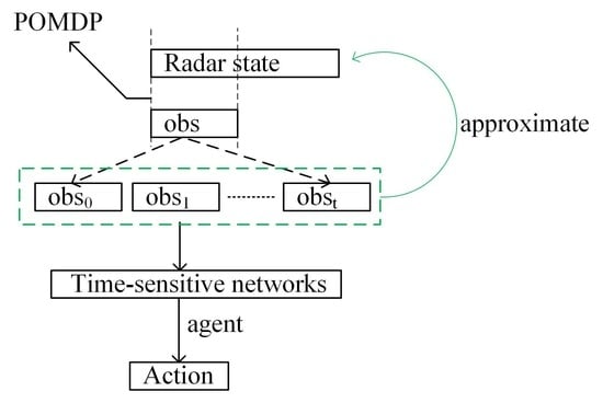
The process of radar frequency hopping against the jammer is constructed as a POMDP, and the partially observable problem is solved by using a radar history observation sequence.

2.

It has been proven that the time-sensitive network has more advantages than the FFN in terms of extracting information from the radar observation sequence.

3.

Optimizing the reward design of the agent helps the reinforcement learning model with LSTM to achieve faster convergence. In a POMDP, the agent relies on historical observations, and each layer of actions and rewards in the observation sequence will impact the agent’s decision. Therefore, the agent’s reward after taking action should not be independent (i.e., the reward design in the MDP is only related to the action of this round), but should rather reflect the connection between the decisions. Therefore, we optimized the reward function to speed up the learning speed of the agent to resist the jammer in sweep mode.

4.

Extensive experiments were carried out to prove the method.

The remainder of this paper is organized as follows: Section 2 introduces the system model of the radar and the jammer; Section 3 presents the interaction model between the radar agent and the jammer; Section 4 provides the simulation results; and Section 5 presents the conclusions.

2. System Model

This paper studies the radar anti-interference problem of pulse-to-pulse frequency hopping. The interference is generated by the jamming device through a frequency-sweeping strategy, which is widely employed as an active attack technique [25]. Next, we will introduce the model of the radar and the jamming device.

2.1. The Signal Model of the Radar

Assuming that the radar transmits N pulses in one coherent processing interval (CPI), and each pulse has a constant pulse repetition interval (PRI), the radar can change the transmitting carrier frequency during the pulses. The mathematical expression for the i-th pulse can be presented as follows:

$$s_i\left(t\right)=u\left(t\right)\exp \left(j2\pi f_{m}t\right)$$

(1)

where $i\in \left\{0,1,\dots ,N-1\right\}$, which represents the i-th pulse in each CPI, $N$ represents the total number of pulses transmitted by the radar in each CPI, and $u\left(t\right)$ represents the envelope function. In addition, $f_m\in \left\{f_0,f_1,\dots ,f_{L-1}\right\}$, which represents the m-th frequency in the frequency space, and $L$ represents the length of the frequency space. $\mathrm{\Delta }f=f_m-f_{m-1}$, which represents that the adjacent carrier frequencies have a fixed step size [26]. The radar has the flexibility to choose any frequency in the frequency space to be the carrier frequency [27,28].

2.2. The Model of the Jammer

Here, the jammer employs a frequency-sweeping strategy to attack the radar. In the environment of the confrontation of the radar and the jammer, we assume that the radar operating bandwidth is large, and that the jammer’s detection capability and the instantaneous frequency bandwidth are restricted. In order to traverse the radar carrier frequency space as quickly as possible, the jammer uses discrete, random, and fast instantaneous frequency measurement technology [29]. We assume that the confrontation scenario is radar sea detection, where the radar detection pulse exceeds 10 μs [30]. The jammer uses the instantaneous frequency measurement with the phase comparison method, and the frequency measurement time of each frequency point is less than 100 ns [29]. It can be seen that the detection of a measurement time made up of 20 frequency points is less than 2 μs for the jammer. To simplify, we assume that the jammer could acquire a lot of frequency point information simultaneously within a PRI. In addition, regarding the problem of the interference and radar carrier frequency space being the same, we follow the literature [17] and assume that the enemy uses an electronic intelligence [31] system to obtain all of the available carrier frequencies of the radar. Overall, we assume that the jammer and the radar operate in the same frequency space, the jamming and radar pulses are synchronized in time, and the jammer is able to detect multiple radar frequencies within one PRI. The working process of the jammer is as follows: Firstly, it scans the frequency space of the radar using the M-sequence method [32], and the M_int carrier frequencies are detected at each PRI. If a radar signal is detected, the jammer immediately emits jamming signals at that frequency in the same PRI, and it will detect the same M_int frequencies at the next PRI. After detecting all of the carrier frequencies, the jammer starts a new turn of detection. If the jammer does not find a radar signal, it will scan the frequencies in the frequency space randomly and select M_tran frequencies, which emit strong suppression jamming signals. When all of the carrier frequencies are scanned, this starts a new turn of emission. From the perspective of the jammer, the frequency space can be divided into the detected carrier frequency space, the currently detecting carrier frequency space, and the upcoming detecting carrier frequency space. The additional random emission function enables the jammer to have the capability to attack both the detected and the undetected frequencies. The strong suppression jamming not only affects the launch frequencies of the jammer, but also suppresses the adjacent frequencies. For instance, when M_tran = 1, and the jamming signal is at frequency f_j, the radar operating at frequencies f_j−1, f_j, and f_j+1 will be affected. In the frequency scanning mode, the jammer is helpless against the target radar in the scanned carrier frequency space, however, strong suppression can compensate for this limitation. Here, we assume that the jammer has strong detection and rapid response capabilities. As long as the M_int frequencies are detected, including the radar working frequency, the jammer can immediately obtain all of the signal parameters of the radar and release interference. In fact, the maximum number of frequencies that the jammer can interfere with in each PRI is $M_{\mathrm{int}}+3\times M_{tran}$.

From the radar’s perspective, the jammer’s characteristics remain unknown. An example of the radar and jammer countermeasures is shown in Figure 1. At the first PRI, the radar was transmitted on the carrier frequency f₆, while the jamming system detected frequencies f₄ and f₇. The jammer did not intercept the radar’s frequency, so it randomly selected frequency f₂, on which there were strong suppression jamming signals. The strong suppression jamming also affected the neighboring frequencies f₁ and f₃. Therefore, the jamming system could interfere with frequencies f₄, f₇, f₁, f₂, and f₃, but not with the radar’s working carrier frequency f₆. As a result, the radar successfully resisted the interference. At the second PRI, the jammer changed its detection frequencies to f₅ and f₆, which included the radar’s working frequency. Here, we assume that the jammer immediately generates interference after discovering the radar signal within the same PRI. Without considering a time delay, we believe that the radar has been interfered with. At the third PRI, because the radar experienced interference in the previous PRI, it changed its transmitting carrier frequency to f₄. The jammer successfully detected the radar’s frequency at the second PRI and then continued to detect frequencies f₅ and f₆ but did not find the radar signal at the third PRI. Consequently, the jammer system emitted strong suppression jamming at frequency f₃, affecting frequencies f₂, f₃, and f₄, which led to the radar being jammed once again. At the fourth PRI, the radar hopped to frequency f₇, and the jammer changed its detection frequencies to f₃ and f₈. Then, the suppression jamming impacted frequencies f₁, f₂, and f₃, which did not include the radar’s working frequency f₇. Consequently, the radar successfully resisted the interference.

3. Interaction Model

The challenge we face when implementing radar adaptive anti-interference is that the radar cannot directly observe the status information of the jammer. The radar only knows whether the current frequency is being interfered with, which means that radar anti-interference is a partially observable problem, and the process of the radar interacting with the jammer is a partially observable Markov decision process, abbreviated as POMDP. Fortunately, we can address this issue by utilizing the historical observation information sequence of the radar. In this section, we first explain the unique nature of the radar’s confrontation with the jammer. Then, a radar anti-jamming model based on reinforcement learning is proposed. Finally, we employ an improved Double-DQN algorithm [33] to solve the radar’s adaptive frequency hopping problem.

3.1. Special Features of Radar Anti-Jamming

The essence of reinforcement learning is interactive learning, which allows the agent to interact with the external environment. The agent perceives the external environment and selects its actions, accordingly, responds to the environment, observes the consequences of its actions, adjusts its action selection mechanism based on the observed outcomes, and ultimately strives to achieve optimal responses to the external environment. An example of the interaction between the radar and the jamming environment is shown in Figure 2. This shows the interaction process between the intelligent agent and the environment. The interaction between the intelligent agents and the environment is also applicable to the process of radar and interference countermeasures. At time t, the radar acts a_t based on the current state s_t and reward r_t, affecting the environment and transferring it to the next state s_t+1, resulting in obtaining the corresponding reward r_t+1. The mathematical foundation of reinforcement learning is MDPs, which can be described using the following key elements [7]:

• A set of states S. Let s_t represent the state of the agent at time t.
• A set of actions A. Let a_t represent the action made by the agent at time t.
• State transition probability:

$$P\left(s_{t+1}|s_1,\dots ,s_t,a_t\right)=P\left(s_{t+1}|s_t,a_t\right).$$

(2)

• Immediate reward function:

$$R_{t+1}=R\left(s_{t+1}|s_t,a_t\right).$$

(3)

At time t, the agent predicts the state transition probability based on the historical state sequence $\left(s_1,\dots ,s_t\right)$ and takes the action a_t. At the same time, it also obtains the reward feedback R_t. Due to the Markov properties [7], state s_t implies that it contains all of the information from s₁ to s_t−1, and the agent can obtain the state transition probability $P\left(s_{t+1}|s_t,a_t\right)$ of s_t+1 to rely on the s_t and a_t. In practical scenarios, the interference environment is unknown to the radar, and the radar is not able to directly perceive the truth state value. Instead, it only has access to the observed value o_t from a radar perspective. However, the observed value o_t only provides partial information about the actual state value of the radar. Consequently, the o_t does not strictly satisfy the Markov property. It does not contain all of the information of the previous observations, indicating that the radar anti-jamming process is a POMDP. It is not sufficient to simply use the o_t as a substitute for s_t to predict the state transition probabilities. To address this problem, a sequence of historical observation information $\left(o_1,\dots ,o_t\right)$ can be utilized to help the agent to better understand its state and make decisions. In this paper, we set that each layer of radar observation data includes the radar’s carrier frequency, the action, and the reward. We combine consecutive layers of observations into matrices in order to approximate the state of the radar. Since the DQN uses an offline reinforcement learning method, we can store the multi-layer observation matrix directly in the replay buffer to assist the agent in training the network.

In Figure 3, using the example of Chinese chess, the differences between the MDP and POMDP models are illustrated under the reinforcement learning framework. In the MDP model, the red agent can observe the position of any chess piece on the board, allowing it to have full knowledge of the agent’s state. The current state of the chessboard is due to the interaction between both of the players and contains all of the historical state information. Therefore, the red agent can play chess solely based on the current state of the chessboard. On the other hand, in the POMDP model, the red agent can only observe the positions of their pieces. They lack information about the opponent’s pieces unless they attack. To make informed decisions, the red agent can rely on the sequence of historical observations to infer the possible positions of their opponent’s pieces and then determine their next move.

Figure 2. The interaction process between the agent and the environment.

Figure 2. The interaction process between the agent and the environment.

3.2. Parameter Design for Reinforcement Learning

In the following section, we will introduce the state, actions, and reward design details of the POMDP model.

• States: During the process of radar anti-interference, the radar perceives the environment by receiving echo signals and utilizes historical observations to infer the true state, enabling it to make appropriate anti-interference decisions. To address this partially observable problem, we define the input state of the intelligent agent as follows:

$$s_t=\left[\begin{array}{c}{o}_{t-1}\\ o_{t-2}\\ ⋮\\ o_{t-k}\end{array}\right]=\left[\begin{array}{c}{f}_{t-1}\\ f_{t-2}\\ ⋮\\ f_{t-k}\end{array}\begin{array}{c}{a}_{t-1}\\ a_{t-2}\\ ⋮\\ a_{t-k}\end{array}\begin{array}{c}{r}_t\\ r_{t-1}\\ ⋮\\ r_{t-k+1}\end{array}\right]$$

(4)

where f_t−k and a_t−k represent the carrier frequency and the action of the radar at time t − k, respectively, and r_t−k+1 represents the corresponding reward. Note that f_t and a_t differ in time by one PRI, and f_t represents the radar carrier frequency at time t, which is the frequency hopping target selected by the agent at time t − 1. a_t represents the carrier frequency index chosen by the agent at time t, and the radar will use the carrier frequency corresponding to a_t to transmit the LFM signal at time t + 1.

• Actions: Actions reflect the agent’s decision-making process. In a CPI, the radar can hop frequencies on any PRI pulse to evade interference. We state that the agent can choose one of the L frequencies in the carrier frequency space as their hopping object.

$$a_t=f_j\in F=\left\{f_1,\dots ,f_L\right\}$$

(5)

Under this definition, the action space of the radar and the jammer is equal to the carrier frequency space F.

• Reward Function: Rewards are used to evaluate the value of the radar agent’s decisions, and the feedback can guide the agent in their learning in the future. Considering the characteristics of the sweep mode, we define the reward function as follows:

$$r_t=r_{st}+r_{at}$$

(6)

with

$$r_{st}=\left\{\begin{array}{c}-{\beta }_0-n_{keep},\\ {\beta }_1\times n_{keep}+{\beta }_2\times n_{anti},\end{array}\right.\begin{array}{c}jammed\\ otherwise\end{array}$$

(7)

and

$$r_{at}=\left\{\begin{array}{c}-c,\\ 0,\end{array}\right.\begin{array}{c}hop\\ otherwise\end{array}$$

(8)

where n_anti represents the number of successive times the radar has not been jammed; n_keep represents the number of successive times the radar has used the current carrier frequency; and ${\beta }_0,{\beta }_1,{\beta }_2$, and c are the hyperparameters. The interference judgment method is similar to the one outlined in the literature [17]. If the carrier frequency of the radar and the jammer collide, we judge that the radar has been interfered with.

The reward function consists of the following two parts: r_st, which represents the reward for entering state s_t, where a positive reward is given when there is no interference, and a penalty is given when interference occurs; and r_at, which represents the reward for taking action a_t, where a penalty is given only when frequency hopping occurs. ${\beta }_0$ is a relatively large parameter compared to ${\beta }_1,{\beta }_2$, and c. It is important to ensure that the agent is punished more heavily when interference occurs so that the agent can focus on learning how to avoid such interference in the future. To help the radar to learn information more quickly from historical observations, we introduce the variables n_anti and n_keep in the definition of the reward function r_st. When the radar is disturbed, a higher value of n_keep results in a greater penalty for the agent. In the case of interference from the sweeping mode of the jammer, if the radar remains on the same frequency for a longer duration, the likelihood of interference increases. Therefore, the radar agent needs to take on a higher risk; consequently, the agent will receive a larger penalty. In the case of successful radar anti-jamming, we incorporate rewards associated with n_anti and n_keep. In the segments in which the radar is not jammed, a higher value of n_anti indicates more times when anti-jamming was successful, and a higher value of n_keep implies a lower number of frequencies used. This means that the better the decision-making ability of the radar agent, the better the reward they receive should be.

3.3. Deep Reinforcement Learning

Given the impracticality of using a table to record large action and state spaces, the DQN addresses the limitation of Q-learning by adopting the idea of function approximation. This utilizes the powerful representation capabilities of neural networks to calculate the value for each input state. With the assistance of modules like experience replay and a target network, the network parameters are updated to train the agent. The rules for Q-learning are as follows [8]:

$$Q\left(s_t,a_t\right)\leftarrow Q\left(s_t,a_t\right)+\alpha \left[r_{t+1}+\gamma \underset{a\in A}{\max } Q\left(s_{t+1},a_{t+1}\right)-Q\left(s_t,a_t\right)\right]$$

(9)

Q-learning utilizes the temporal difference (TD) learning target $r_{t+1}+\gamma \max Q\left(s_{t+1},a_{t+1}\right)$ to update $Q\left(s_t,a_t\right)$. The objective of this is to make the $Q\left(s_t,a_t\right)$ approach the TD learning target. Therefore, the loss function of the Q-network in DQN can be constructed as follows [9]:

$${\omega }^{\ast }=\arg \underset{\omega }{\min }\frac{1}{2N}{\displaystyle \sum _{i=1}^N\left[Q_{\omega }\left(s_t^i,a_t^i\right)-\right.}{\left.\left(r_{t+1}^i+\gamma \underset{a_{t+1}}{\max } Q_{{\omega }^{-}}(s_{t+1}^i,a_{t+1})\right)\right]}^2$$

(10)

The learning objective, which is computed by the target network, can be expressed in the following form:

$$\underset{a_{t+1}}{\max } Q_{{\omega }^{-}}\left(s_{t+1},a_{t+1}\right)\to Q_{{\omega }^{-}}\left(s_{t+1},\arg \underset{a_{t+1}}{\max } Q_{\omega }\left(s_{t+1},a_{t+1}\right)\right)$$

(11)

where $\underset{}{\max } Q_{{}^{\omega -}}\left(s_{t+1},a_{t+1}\right)$ is decomposed into two parts, as follows: one part involves selecting the optimal action $a^{\ast }=\underset{}{\arg \max }{Q}_{\omega }\left(s_{t+1},a_{t+1}\right)$ for the next state s_t+1, and the second part then calculates the value of this action $Q_{\omega -}\left(s_{t+1},a^{\ast }\right)$. The Double DQN algorithm utilizes two independent neural networks to estimate these two parts. One network is used to select the action with the highest value based on its output, while the other network is used to calculate the value of the action [33]. Using two separate networks effectively addresses the issue of overestimation in Q-value estimation by the neural networks.

In deep reinforcement learning, the traditional Q-network is typically constructed as a multi-layer perceptron (MLP) consisting of multiple fully connected layers. This structure is not sensitive to the temporal dimension and is suitable for scenarios where time series information is not crucial, just as in the MDP. However, in the case of radar anti-jamming, we cannot ignore the historical information. Fortunately, we have LSTM as a classic neural network model that is sensitive to time sequences [34]. LSTM consists of forget gates, memory gates, and output gates. The forget gates selectively forget the past information based on the previous time step’s output and the current input, allowing LSTM to maintain important information in its long-term memory. The memory gates extract the relevant information from the current time step, while the output gates compute the information to output at the current time step. In Double-DQN, we only replace the first fully connected layer (FC) in the Q-network with LSTM to make it sensitive to the time series.

The Q-network with an LSTM structure is depicted in Figure 4. The input consists of a $3\times 3$ matrix formed by the agent’s historical observations. Then, it is processed by the LSTM network to extract the relevant information, where the input size of LSTM is 3, the output size is 16, and the number of layers is 1. The $3\times 16$ relevant information will be flattened to $1\times 48$ hidden information, and the fully connected layers are used to select the optimal action and compute the value. Subsequent experiments have demonstrated that LSTM, and other time-sensitive networks, such as a Recurrent Neural Network (RNN) [35] and Gate Recurrent Unit (GRU) [36], can achieve excellent performance in tackling the partially observable problem.

In fact, this time-sensitive ability originates from a distinctive network structure, in which the output of the current network not only depends on the current input, but also on the network output at the previous moment. We take the radar observation sequence as the input, and each layer of the observations corresponds to a time step. We expand these networks in the time dimension to form network units corresponding to the cells in Figure 4. In the figure, the green input and the previous yellow cell output affect the green cell output. For the RNN, the previous cell output is weighted and fused with the current information to form the cell output. The LSTM network is more sophisticated, including forgetting gates, memory gates, and output gates. The forgetting gate realizes the fusion of the previous cell output and the input of the moment. The memory gate focuses on the input information of the current cell. The output gate integrates the forgetting gate, the memory gate, and the current information to form the output. The GRU simplifies the gating structure of LSTM and combines the memory gate and the forgetting gate into one.

3.4. The Process between the Radar and Jammer

In the previous sections, we designed the working modes of the radar and the jammer and selected the Double-DQN algorithm to solve the radar anti-interference problem. We optimized the states, reward function, and network. Next, we will present the multi-round interaction process between the radar agent and the jammer, as shown in Algorithm 1.

Algorithm 1: The Process between the Radar and Jammer.

INITIALIZE. H: replay-buffer; ω: network-parameters     INITIALIZE. ω−: copy of ω; N−: target update cycle     INITIALIZE. Operating parameters of radars and jammers.     for each CPI do    Initialize the radar observation matrix as the initial state of the agent    for each pulse do     Choose according to the greedy algorithm     The jammer emits jamming in sweep mode     According to st and at, obtain st+1, rt+1     Store transition (st, at, rt+1, st+1) in H      st ← st+1         end for   Sample minibatch data from H randomly   Obtain $a^{\max }=\left(s_{t+1};\omega \right)=\arg {\max }_{a_{t+1}}Q\left(s_{t+1},a_{t+1};\omega \right)$   Calculate TD learning target yj   Update network parameters with ${‖y_j-Q\left(s,a;\omega \right)‖}^2$   Update the greedy parameters   Replace target parameters ω− ← ω every N− steps    end for

4. Results

In this section, we present the simulation results in order to validate the performance of the improved reinforcement learning model. The simulation results cover the adaptive frequency hopping anti-interference performance, the impact of the time-sensitive network models, the effectiveness of the reward design, and the influence of the layers of historical observations. The network structure design, the hyperparameters of the Double-DQN, and the radar and jammer parameters are summarized in

Table 1. Design of Q-network structure.

Layer	Input Size	Output Size
LSTM	$3\times 3$	$3\times 16$
Flatten	$3\times 16$	$1\times 48$
FC	$1\times 48$	$1\times 100$

,

Table 2. Hyperparameters of Double-DQN.

Parameter	Value
Episodes	500
Number of pulses in a CPI	64
Discount rate	0.98
Learning rate	0.001
$\epsilon$-greedy increment	0.1
Target update	10
Buffer size	2048
Minimal size	512
Batch size	64

, and

Table 3. Parameters of the radar and the jammer.

Parameter	Value
Number of frequencies L	100
Hopping cost c	1
Mtran	2
Mint	20
Historical observation layers	3
${\beta }_0$	5
${\beta }_1$	0.2
${\beta }_2$	0.1

, respectively. The greedy parameter $\epsilon$ in Table 1 rapidly decreased from 0.1 to 0 during the iterations. If the $\epsilon$ remains unchanged, the training results will irreversibly deteriorate after a certain number of iterations. The following simulation results were obtained by averaging over 500 Monte Carlo realizations [37].

4.1. The Performance of Radar Adaptive Frequency Hopping

First, we will validate the effectiveness of introducing the LSTM network and the multi-layer historical observations to improve the radar anti-interference capability. Figure 5 displays the curve of P_NI (i.e., the successful anti-interference ratio within a CPI), which directly reflects the radar anti-interference performance. Figure 6 represents the frequency hopping times within a CPI. In Figure 5 and Figure 6, the ‘LSTM + History’ represents our proposed approach, which introduces historical observation information and an LSTM network. In the figure, as in the training, the P_NI of the ‘LSTM + History’ gradually increases and eventually stabilizes. It shows a high success ratio of 0.92 for anti-interference, with 42 frequency jumps. ‘Random’ represents the radar without using reinforcement learning, and the working frequency was randomly selected. Due to the lack of learning capability, this curve remains relatively stable in multiple repeated experiments. The P_NI remains at about 0.76, and the frequency hopping times remain at about 64. When comparing ‘Random’, it is evident that our proposed model significantly improves the anti-interference capability. The P_NI is increased by 0.16, and the frequency hopping times are reduced by 20. This indicates that our model achieves a better anti-interference performance with fewer frequency hops.

‘MLP + History’ is represented using two FC layers to extract the historical observation information. After stabilization, the P_NI is 0.73, and the number of frequency hops is 53. Comparing the ‘LSTM + History’, the P_NI decreases by 0.19, and the number of frequency hops increases by 11. Because MLP networks only extract information from an overall perspective and cannot capture the information between the individual layers of the observations, this means that the MLP is not sensitive to the time dimension information. On the other hand, LSTM can exploit the hidden information when dealing with the time series. Based on these results, we can see the advantages of LSTM in handling multi-layer historical observations.

‘LSTM’ represents the agent using a single layer of observations as an input to the LSTM network. After stabilization, the P_NI is 0.847, and the frequency hopping times remain at about 47. Compared with ‘LSTM + History’, the P_NI decreases by 0.073, and the hopping times increase by 5. The results show that LSTM undergoes a certain degree of decline regarding anti-interference performance and convergence speed without the help of the historical information.

‘MLP’ represents the agent that uses only a single-layer observation as the input, and the Q-network structure consists of two FC layers, which is a common approach used in previous studies [16,17,19]. After stabilization, the P_NI is 0.6, and the number of frequency hops is 44. When comparing ‘MLP + History’, by removing the three layers of historical observations, the P_NI decreases by 0.13. The multiple layers of historical observations improve the radar anti-interference to some extent. However, due to the limitations of the MLP structure, these results are still not good.

Through the above analysis, we can conclude that, in a POMDP, introducing multiple layers of historical observations can improve the anti-jamming performance. When combined with LSTM to extract time dimension information, the radar can more accurately learn the work of the jammer, resulting in a significant improvement in anti-interference.

4.2. The Effects of a Time-Sensitive Network

In the previous section, we verified the excellent performance achieved by combining LSTM with historical observations. Next, we will show that this effect is not due to the size of the model, but rather the time sensitivity of the network.

When translating from one language to another, the order of the words significantly impacts the meaning of a sentence. Therefore, Natural Language Processing (NLP) must consider the sequential order of the words and uncover the information hidden within the temporal sequence [38]. This similarity between NLP and our problem suggests that we can leverage the other classic models used in NLP, such as the RNN and GRU, to evaluate the ability of time-sensitive networks to solve POMDPs.

The RNN is one of the most classic models in NLP. It introduces the idea that the current output of a network depends on the current input and the previous hidden layer output so that the network can be sensitive to time order [35]. The disadvantage of the RNN is that it struggles to remember the content at the beginning of a sequence when it is very long. However, memory loss is not a concern, due to the short observation sequences of the agent. The GRU is a simplification of LSTM. It combines the forgetting and input gates into an update gate and merges the unit and hidden state. Therefore, the GRU can simultaneously perform the operations of forgetting and selectively remembering [36].

As shown in Figure 7 and Figure 8, we also selected two other classic networks, the RNN and the GRU, to validate the superiority of time-sensitive networks in handling POMDPs. The model parameters of these networks are consistent with LSTM. We also increased the hidden layers of the MLP in Figure 5 and observed the impact of simply increasing the model size. The MLP in Figure 5 increases from two fully connected layers to four layers, making it MLP4. The curves ‘GRU + History’ and ‘RNN + History’ represent the GRU and RNN network models, respectively. Through continuous learning, these two models were also able to achieve a P_NI of 0.92, demonstrating significant improvement compared to the MLP model. In terms of the frequency hopping number shown in Figure 8, LSTM outperformed the GRU and the RNN. On the other hand, ‘MLP4 + History’ represents a four-layer FC network, with a maximum P_NI of only 0.6, which results in no improvement compared to the performance of the two-layer FC structure shown in Figure 5. From the perspective of the model parameters, the MLP4 structure exceeds the LSTM, GRU, and RNN networks, but this does not bring about performance improvements. Based on the experimental results shown in Figure 5 and Figure 7, we believe that the key to helping the agent to counteract interference is the extraction of temporal information from historical observations rather than the size of the network.

4.3. The Effects of Reward

Although the LSTM model achieved good results, it had a slow convergence speed. To help the radar to counter the interference from the jammer more quickly, we introduced the concept of ‘successive times’ in the reward function design. Specifically, we incorporated the idea of successive n_anti times without interference and successive n_keep times on the same carrier frequency. In this section, we will verify the improvement in the learning speed with the optimized reward design.

We visually demonstrate the effect of improving the convergence speed in pictures. We conducted a series of validations using the LSTM model. As shown in Figure 9, the curve labeled ‘reward’ represents the reward design proposed in this paper, while the curve labeled ‘no’ represents the case where the intelligent agent uses a fixed reward. It is evident that the reward design in this paper leads to faster convergence. At 74 iterations, the difference in P_NI between the two approaches is as high as 0.14. With a fixed reward design, it took 281 iterations for the radar agent to reach a P_NI of 0.92. However, when we incorporated the concept of ‘successive times’ in the reward formulation, the number of iterations decreased to 185, reducing it by 96 iterations. This indicates that using ‘successive times’ in the reward design leads to an improvement in the convergence speed, and, when we only introduced n_anti and n_keep in the observations (i.e., the ‘observation’ label), the number of iterations increased to 383, adding 107 iterations. This indirectly indicates that the LSTM network can extract information from the historical observations, and the redundant information slows down the network analysis. When we incorporated ‘successive times’ in both the reward design and the observations (i.e., the ‘reward + observation’ label), the iterations reduced to 240, and the convergence speed of the agent also improved. This suggests that, in terms of accelerating the convergence speed of the agent in this paper, the reward design is more important.

As the jammer operates in a frequency-sweeping mode, the longer the radar stays on the same frequency, the more susceptible it is to interference. At the same time, the radar uses fewer frequencies to obtain a higher P_NI, which means that better anti-jamming decisions are made and the received reward is better. This reward design stimulates the agent to learn the jammer’s behaviors, ultimately achieving a balance between the risks and the rewards. Although the optimized design did not improve the radar’s anti-interference performance, it did accelerate the learning speed of the intelligent agent.

4.4. The Influence of the Number of Observation Layers

In the previous chapters, we used a three-layer history observation as the state of the intelligent agent to assist the radar in making adaptive decisions and achieving good results. Next, based on LSTM, we examine the impact of the different layers of historical observations on the state of the intelligent agent.

As shown in Figure 10, the P_NI reaches 0.905 when using nine layers of historical observations. The P_NI is the lowest, at 0.847, when using only one layer of observation. When the number of layers of historical observations is less than three, the performance is poor, due to the lack of temporal information. Notably, due to the introduction of the time dimension, the improvement in the performance is most significant when the number of layers of historical observations increases from one to two. The peak performance is 0.922 when there are three layers of historical observations. However, increased layers of historical observations do not always lead to a better performance. When using excessive layers, the temporal dimension may span multiple scan cycles of the jammer. For example, in the case of $M_{\mathrm{int}}=20$, $M_{trans}=2$, and $L=100$, the interference source can disrupt all of the frequencies within 4–5 PRI. In this paper, the jammer adopts a frequency-sweep mode for detection. In each frequency-sweep cycle, due to the differences in the agent actions during the training, the jammer’s detection time for some carrier frequencies, the timing of performing strong suppression interference, and the frequency-sweep cycle time will be different. In addition, the jamming environment is unknown to the radar, and the radar can only infer the jammer’s strategy from its observation data. The data at different sweep periods contain slightly different jamming strategies, which increases the complexity of the radar learning from the observation sequence and may even be misleading. Therefore, the observations from other scan cycles could not provide information for the current prediction and may have a negative impact. Therefore, using five or more layers of historical observations results in a noticeable drop in performance.

4.5. Comparison of Method

In studies [16,17,39,40], the researchers typically used the total SINR within a CPI (or detection probability related to the total SINR) as the evaluation metric for the radar’s anti-jamming performance. Specifically, they integrated the echo pulses that remained free from interference during the CPI, performed a coherent integration with the same carrier frequency, and then conducted an incoherent integration on the various coherent results. Therefore, the total SINR in a CPI is related to the number of hops and the P_NI.

These methods generally improve the anti-jamming performance compared to selecting the frequency randomly. Comparing the random method, the reinforcement learning approach employing an MLP-based Q-network can significantly reduce the radar hopping frequency times, while the P_NI increases little but obtains a high total SINR. This is because the gain from the incoherent integration is less than that from the coherent integration [41]. With the number of successful anti-interferences held constant, reducing the hopping frequency times results in a higher proportion of coherent components, thereby producing a higher total SINR. Therefore, in the results of this paper, we directly presented the P_NI and hopping frequency times as two key metrics that could clearly show the radar anti-jamming performance brought about by reinforcement learning.

Figure 11 presents the total SINR of the above methods within one CPI. For ease of calculation and analysis, we assume that the SINR of the radar echo within one PRI is a fixed value when the radar successfully counters interference. After collecting the echo data of a CPI, the radar makes statistics on the anti-interference status of each PRI. If the radar can achieve anti-interference successfully, we record the PRI carrier frequency and SINR value, otherwise, we discard the data. After completing the CPI statistics, we perform coherent integration on the data with the same carrier frequency and then perform incoherent integration on the coherent results of each carrier frequency to obtain the total SINR of a CPI [17]. We assume that the recorded results of the two CPIs are [f₁, f₁, f₂] and [f₁, f₂, f₃], respectively. Since the coherence is greater than the incoherence gain, the frequency hopping strategy [f₁, f₁, f₂] will be greater than another strategy [f₁, f₂, f₃] in terms of the total SINR value when we fix the SINR value of each PRI. It is foreseeable that, although the random frequency hopping method may have a higher P_NI, it also uses more types of carrier frequencies, which results in a smaller proportion of coherent integration with a CPI (even if only performing non-coherent integration). Therefore, we may obtain a lower total SINR when we use the random method. The labels in Figure 11a,b correspond to those in Figure 5 and Figure 7. The reinforcement learning methods shown in Figure 11a,b can achieve convergence. In Figure 11a, the total SINR value after convergence for each curve is as follows: ‘LSTM + History’ is 33, ‘MLP + History’ is 23, ‘MLP’ is 20, and ‘Random’ is 8. Under the total SINR metric for one CPI, we conclude that, while ‘MLP + History’ and ‘MLP’ methods are inferior to the ‘LSTM + History’ method, they each achieve significant improvements of 15 and 12, respectively, compared to the ‘Random’ method. Additionally, they exhibit faster convergence, typically achieving convergence within around ten episodes. In fact, as shown in Figure 5, the ‘MLP + History’ and ‘MLP’ methods do not yield improvements in the P_NI relative to ‘Random’. Combining this with Figure 6, where the ‘Random’ radar mode maintains hopping frequencies, we can see that the increase in the total SINR is due to reinforcement learning based on the MLP networks, which reduces the radar frequency hopping times, thereby increasing the weight of the coherent integration in a CPI, resulting in a larger total SINR. The results shown in Figure 11b further validate our analysis. Despite the fact that, in Figure 7, the P_NI results using the LSTM, GRU, and RNN networks are similar, in Figure 8, the LSTM + History mode has the fewest frequency hops and consequently achieves the highest total SINR. Despite the higher frequency hopping times that come with the GRU and RNN methods, their substantial improvements in successfully countering interference compared to the MLP4 network result in a higher total SINR value.

In [16,17], even though the carrier frequency space was extensive, the action space of the agent included only the following two choices: ‘h’, denoting the radar frequency hopping action and randomly choosing the carrier frequency from the carrier frequency space, and ‘s’, indicating that the radar would stay on the current carrier frequency. Although these studies introduced the idea of reinforcement learning, they still randomly selected the frequency hopping target. In contrast, the action space for the radar agent in this paper is identical to the carrier frequency space, resulting in a more intelligent selection of the carrier frequency.

Furthermore, researchers have also tried to enhance the Q-network in deep reinforcement learning. In [36], they replaced the MLP of a Q-network with a CNN. However, the CNN is not a time-sensitive network; moreover, it floats the probability curve, and its range is even as high as 0.5. In contrast, the Q-network in this paper uses time-sensitive networks and has a more stable effect. After the probability curve converges, the floating range does not exceed 0.02.

5. Conclusions

In this paper, we used reinforcement learning to solve the problem of adaptive frequency hopping for radar anti-jamming in an unknown environment. We analyzed the process of the radar’s interaction with the jammer and modeled it as a POMDP. In the POMDP model, the radar could only access partial observation information. To address this problem, we introduced multi-layer historical observations and time-sensitive networks. We observed that the convergence speed of the agent was slow when using fixed rewards for each step. To overcome this issue, we optimized the reward function by considering the interdependence of the radar’s decisions, which sped up the learning process. The simulation results demonstrate the rationality of optimizing the intelligent agent’s state representation, network architecture, and reward function. Although the experiments in this paper were conducted in a simplified environment, we believe that it is a successful attempt to solve the partially observable problems and help the radar to adaptively counteract the jammer in the POMDP model. In addition, the reward function used in this paper has limitations, because its design relies on the sweep mode of the jammer. The reward function may need to be redesigned when the jammer adopts a different jamming strategy. However, more importantly, we should consider the impact of historical decisions on the reward of this round when redesigning the reward function in the POMDP.

References

1. Skolnik, M.I. Radar Handbook; McGraw-Hill Education: Berkshire, UK, 2008. [Google Scholar]
2. Li, Y.; Huang, T.; Xu, X.; Liu, Y.; Wang, L.; Eldar, Y.C. Phase transitions in frequency agile radar using compressed sensing. IEEE Trans. Signal Process. 2021, 69, 4801–4818. [Google Scholar] [CrossRef]
3. Qin, Z.; Zhou, X.; Zhang, L.; Gao, Y.; Liang, Y.-C.; Li, G.Y. 20 years of evolution from cognitive to intelligent communications. IEEE Trans. Cogn. Commun. Netw. 2019, 6, 6–20. [Google Scholar] [CrossRef]
4. Krishnamurthy, V.; Angley, D.; Evans, R.; Moran, B. Identifying cognitive radars-inverse reinforcement learning using revealed preferences. IEEE Trans. Signal Process. 2020, 68, 4529–4542. [Google Scholar] [CrossRef]
5. Wang, L.; Peng, J.; Xie, Z.; Zhang, Y. Optimal jamming frequency selection for cognitive jammer based on reinforcement learning. In Proceedings of the 2019 IEEE 2nd International Conference on Information Communication and Signal Processing (ICICSP), Weihai, China, 28–30 September 2019; pp. 39–43. [Google Scholar]
6. Apfeld, S.; Charlish, A.; Ascheid, G. Modelling, learning and prediction of complex radar emitter behaviour. In Proceedings of the 2019 18th IEEE International Conference On Machine Learning And Applications (ICMLA), Boca Raton, FL, USA, 16–19 December 2019; pp. 305–310. [Google Scholar]
7. Sutton, R.S.; Barto, A.G. Reinforcement Learning: An Introduction; MIT Press: Cambridge, MA, USA, 2018. [Google Scholar]
8. Watkins, C.J.C.H. Learning from Delayed Rewards. Ph.D. Thesis, Cambridge University, Cambridge, UK, 1989. [Google Scholar]
9. Mnih, V.; Kavukcuoglu, K.; Silver, D.; Rusu, A.A.; Veness, J.; Bellemare, M.G.; Graves, A.; Riedmiller, M.; Fidjeland, A.K.; Ostrovski, G. Human-level control through deep reinforcement learning. Nature 2015, 518, 529–533. [Google Scholar] [CrossRef] [PubMed]
10. Schulman, J.; Wolski, F.; Dhariwal, P.; Radford, A.; Klimov, O. Proximal policy optimization algorithms. arXiv 2017, arXiv:1707.06347. [Google Scholar]
11. Silver, D.; Lever, G.; Heess, N.; Degris, T.; Wierstra, D.; Riedmiller, M. Deterministic policy gradient algorithms. In Proceedings of the International Conference on Machine Learning, Beijing, China, 21–26 June 2014; pp. 387–395. [Google Scholar]
12. Haarnoja, T.; Zhou, A.; Abbeel, P.; Levine, S. Soft actor-critic: Off-policy maximum entropy deep reinforcement learning with a stochastic actor. In Proceedings of the International Conference on Machine Learning, Jinan, China, 19–21 May 2018; pp. 1861–1870. [Google Scholar]
13. Ak, S.; Brüggenwirth, S. Avoiding interference in multi-emitter environments: A reinforcement learning approach. In Proceedings of the 2020 17th European Radar Conference (EuRAD), Utrecht, The Netherlands, 13–15 January 2021; pp. 262–265. [Google Scholar]
14. Zheng, Z.; Li, W.; Zou, K. Airborne Radar Anti-Jamming Waveform Design Based on Deep Reinforcement Learning. Sensors 2022, 22, 8689. [Google Scholar] [CrossRef] [PubMed]
15. Liu, K.; Lu, X.; Xiao, L.; Xu, L. Learning based energy efficient radar power control against deceptive jamming. In Proceedings of the GLOBECOM 2020-2020 IEEE Global Communications Conference, Taipei, Taiwan, 7–11 December 2020; pp. 1–6. [Google Scholar]
16. Yi, W.; Yuan, Y. Reinforcement learning-based joint adaptive frequency hopping and pulse-width allocation for radar anti-jamming. In Proceedings of the 2020 IEEE Radar Conference (RadarConf20), Florence, Italy, 21–25 September 2020; pp. 1–6. [Google Scholar]
17. Yi, W.; Varshney, P.K. Adaptation of Frequency Hopping Interval for Radar Anti-Jamming Based on Reinforcement Learning. IEEE Trans. Veh. Technol. 2022, 71, 12434–12449. [Google Scholar]
18. Ak, S.; Brüggenwirth, S. Avoiding jammers: A reinforcement learning approach. In Proceedings of the 2020 IEEE International Radar Conference (RADAR), Washington, DC, USA, 28–30 April 2020; pp. 321–326. [Google Scholar]
19. Li, K.; Jiu, B.; Liu, H.; Liang, S. Reinforcement learning based anti-jamming frequency hopping strategies design for cognitive radar. In Proceedings of the 2018 IEEE International Conference on Signal Processing, Communications and Computing (ICSPCC), Qingdao, China, 14–16 September 2018; pp. 1–5. [Google Scholar]
20. Jiang, W.; Ren, Y.; Wang, Y. Improving anti-jamming decision-making strategies for cognitive radar via multi-agent deep reinforcement learning. Digit. Signal Process. 2023, 135, 103952. [Google Scholar] [CrossRef]
21. Geng, J.; Jiu, B.; Li, K.; Zhao, Y.; Liu, H.; Li, H. Radar and Jammer Intelligent Game under Jamming Power Dynamic Allocation. Remote Sens. 2023, 15, 581. [Google Scholar] [CrossRef]
22. Kaelbling, L.P.; Littman, M.L.; Cassandra, A.R. Planning and acting in partially observable stochastic domains. Artif. Intell. 1998, 101, 99–134. [Google Scholar] [CrossRef]
23. Hausknecht, M.; Stone, P. Deep recurrent q-learning for partially observable mdps. In Proceedings of the 2015 AAAI Fall Symposium Series, Austin, TX, USA, 25–30 January 2015. [Google Scholar]
24. Li, K.; Jiu, B.; Wang, P.; Liu, H.; Shi, Y. Radar active antagonism through deep reinforcement learning: A Way to address the challenge of mainlobe jamming. Signal Process. 2021, 186, 108130. [Google Scholar] [CrossRef]
25. Li, N.-J.; Zhang, Y.-T. A survey of radar ECM and ECCM. IEEE Trans. Aerosp. Electron. Syst. 1995, 31, 1110–1120. [Google Scholar]
26. Axelsson, S.R. Analysis of random step frequency radar and comparison with experiments. IEEE Trans. Geosci. Remote Sens. 2007, 45, 890–904. [Google Scholar] [CrossRef]
27. Antonik, P.; Wicks, M.C.; Griffiths, H.D.; Baker, C.J. Frequency diverse array radars. In Proceedings of the 2006 IEEE Conference on Radar, Verona, NY, USA, 24–27 April 2006; p. 3. [Google Scholar]
28. An, P.; Shang, Z.; Yan, S.; Wang, D. Design Method Of Frequency-Agile Radar Frequency Hopping Sequence Based On CNN Network And Chaotic Sequence. In Proceedings of the 2022 International Conference on Big Data, Information and Computer Network (BDICN), Sanya, China, 20–22 January 2022; pp. 702–707. [Google Scholar]
29. Wei-Feng, Z.; Xin-Ling, G.; Jian-Peng, Z. Instantaneous Frequency Measurement Interferometer by the Phase Comparison Method. Sci. Technol. Vis. 2016, 299, 301. (In Chinese) [Google Scholar] [CrossRef]
30. Liu, N.; Dong, Y.; Wang, G.; Ding, H.; Huang, Y.; Guan, J.; Chen, X.; He, Y. Sea-detecting X-band Radar and Data Acquisition Program. J. Radars 2019, 8, 656. (In English) [Google Scholar] [CrossRef]
31. Free, D.; Norwood, M.; House, A. Electronic Warfare in the Information Age; Artech House Inc.: Norwood, MA, USA, 1999. [Google Scholar]
32. Golomb, S.W.; Gong, G. Signal Design for Good Correlation: For Wireless Communication, Cryptography, and Radar; Cambridge University Press: Cambridge, UK, 2005. [Google Scholar]
33. Van Hasselt, H.; Guez, A.; Silver, D. Deep reinforcement learning with double q-learning. In Proceedings of the AAAI Conference on Artificial Intelligence, Phoenix, AZ, USA, 12–17 February 2016. [Google Scholar]
34. Hochreiter, S.; Schmidhuber, J. Long short-term memory. Neural Comput. 1997, 9, 1735–1780. [Google Scholar] [CrossRef] [PubMed]
35. Zaremba, W.; Sutskever, I.; Vinyals, O. Recurrent neural network regularization. arXiv 2014, arXiv:1409.2329. [Google Scholar]
36. Chung, J.; Gulcehre, C.; Cho, K.; Bengio, Y. Empirical evaluation of gated recurrent neural networks on sequence modeling. arXiv 2014, arXiv:1412.3555. [Google Scholar]
37. Rubinstein, R.Y.; Kroese, D.P. Simulation and the Monte Carlo Method; John Wiley & Sons: Hoboken, NJ, USA, 2016. [Google Scholar]
38. Chowdhary, K.; Chowdhary, K. Natural language processing. Fundam. Artif. Intell. 2020, 603–649. [Google Scholar] [CrossRef]
39. Geng, J.; Jiu, B.; Li, K.; Zhao, Y.; Liu, H. Reinforcement Learning Based Radar Anti-Jamming Strategy Design against a Non-Stationary Jammer. In Proceedings of the 2022 IEEE International Conference on Signal Processing, Communications and Computing (ICSPCC), Xi’an, China, 25–27 October 2022; pp. 1–5. [Google Scholar]
40. Li, K.; Jiu, B.; Liu, H. Deep q-network based anti-jamming strategy design for frequency agile radar. In Proceedings of the 2019 International Radar Conference (RADAR), Toulon, France, 23–27 September 2019; pp. 1–5. [Google Scholar]
41. Marcum, J. A statistical theory of target detection by pulsed radar. IRE Trans. Inf. Theory 1960, 6, 59–267. [Google Scholar] [CrossRef]
Figure 1. An example of jammer and radar countermeasures, where L = 8, Mint = 2, and Mtran = 1. The small blue triangle represents the working carrier frequency of the radar, the yellow block represents the detection frequency of the jammer, the small red circle represents the center frequency of the strong suppression interference generated by the jammer, and the pink block represents the frequency affected by the suppression interference.
Remotesensing 15 05467 g001
Figure 3. The different agent perspectives between the MDP and POMDP models. In the MDP model, the red agent can observe the position of any chess piece on the board. In the POMDP model, the red agent can only ascertain their own piece positions. (a) MDP; (b) POMDP.
Remotesensing 15 05467 g003
Figure 4. Q-network with LSTM structure. Color was used to distinguish different observation layers. The radar’s historical observation matrix is used as the input, which is processed through a single LSTM layer to extract information. Then, it is flattened and fed into an FC layer.
Remotesensing 15 05467 g004
Figure 5. The impact of network and historical observation information on PNI.
Remotesensing 15 05467 g005
Figure 6. The impact of network and historical observation information on frequency hopping times within a CPI.
Remotesensing 15 05467 g006
Figure 7. The PNI of time-sensitive network and MLP4.
Remotesensing 15 05467 g007
Figure 8. The frequency hopping times of the network.
Remotesensing 15 05467 g008
Figure 9. Number of iterations for PNI to reach 0.92. The label represents the corresponding design of the label using nanti and nkeep.
Remotesensing 15 05467 g009
Figure 10. Influence of different historical observation layers on radar performance.
Remotesensing 15 05467 g010
Figure 11. To evaluate the performance of each method based on the total SINR in one CPI, the labels of (a,b), respectively, correspond to those in Figure 5 and Figure 7. (a) The impact of network and historical observation information on total SINR. (b) The total SINR of the time-sensitive network and MLP4.
Remotesensing 15 05467 g011