
Similarity and Change Detection of Relief in a Proglacial River Valley (Scott River, SW Svalbard)


Abstract
:1. Introduction
- (i)
- to obtain quantitative information on the rate, magnitude and directions of contemporary relief reshaping of a small proglacial valley under conditions of rapid valley glacier retreat;
- (ii)
- to develop a typology and to map the valley floor forms using geomorphons;
- (iii)
- to undertake a similarity analysis of the valley floor surface and a separation of the relatively homogeneous segments for each measurement season;
- (iv)
- to undertake a similarity analysis of valley floor landforms and an estimation of their variability over a three-year period.
2. Materials and Methods
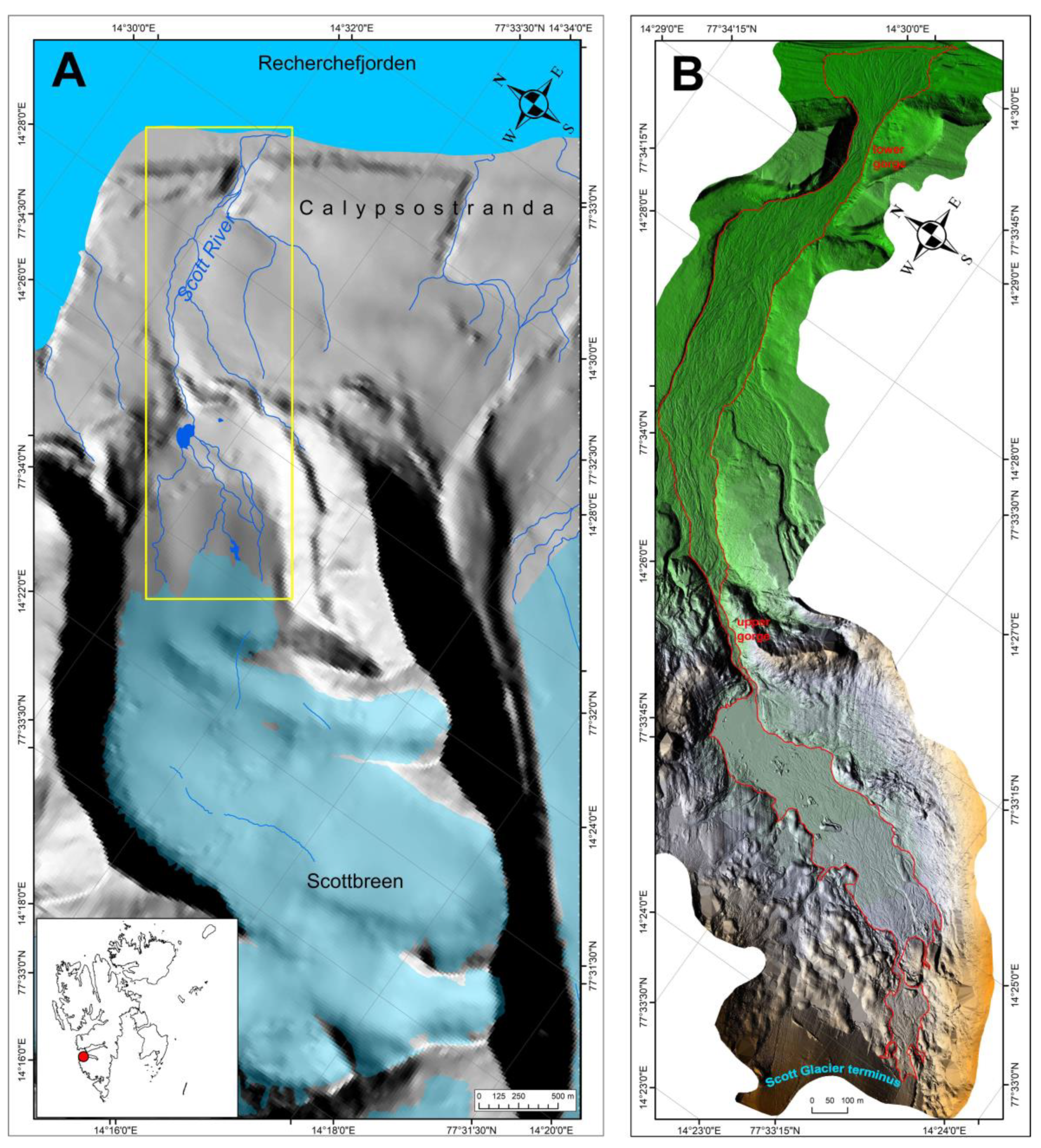
2.1. Study Area
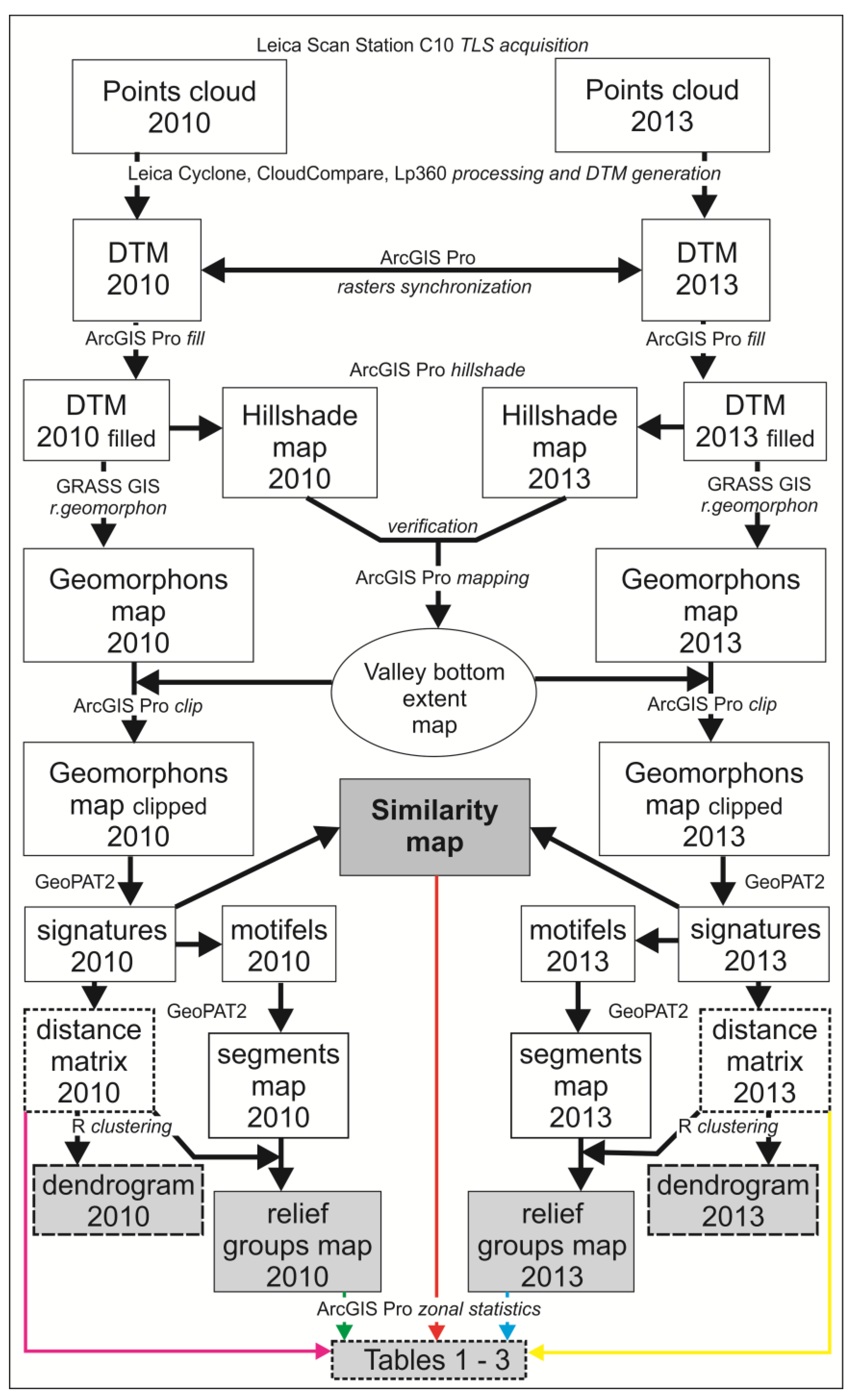
2.2. TLS Scanning (Surveying)
2.3. Postprocessing and DTM Generation
2.4. Geomorphon Maps, Relief Clustering and Similarity
3. Results
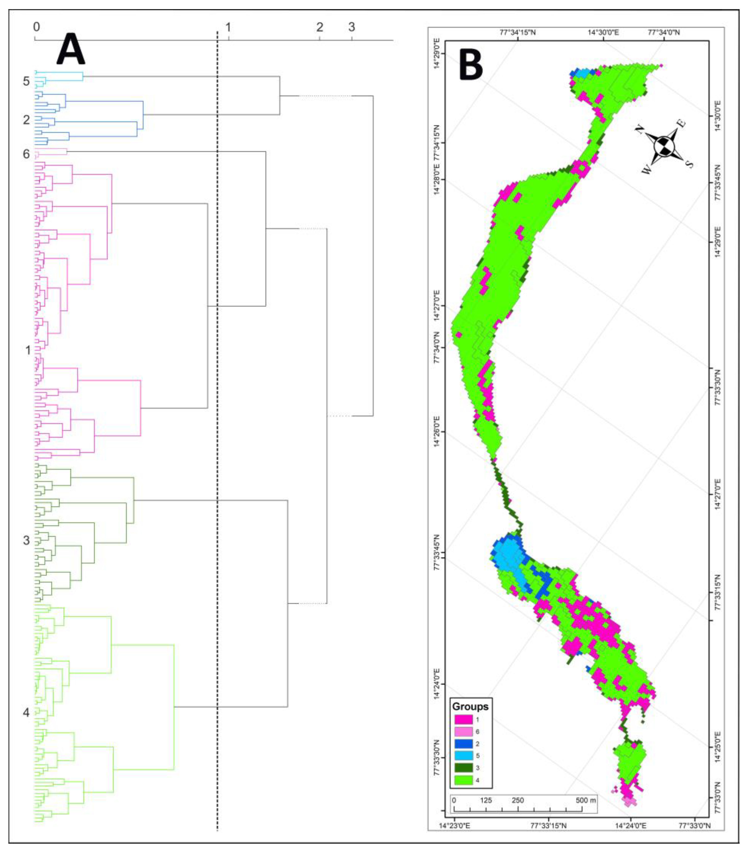
3.1. Relief Classes
3.1.1. The Situation in 2010
3.1.2. The Situation in 2013
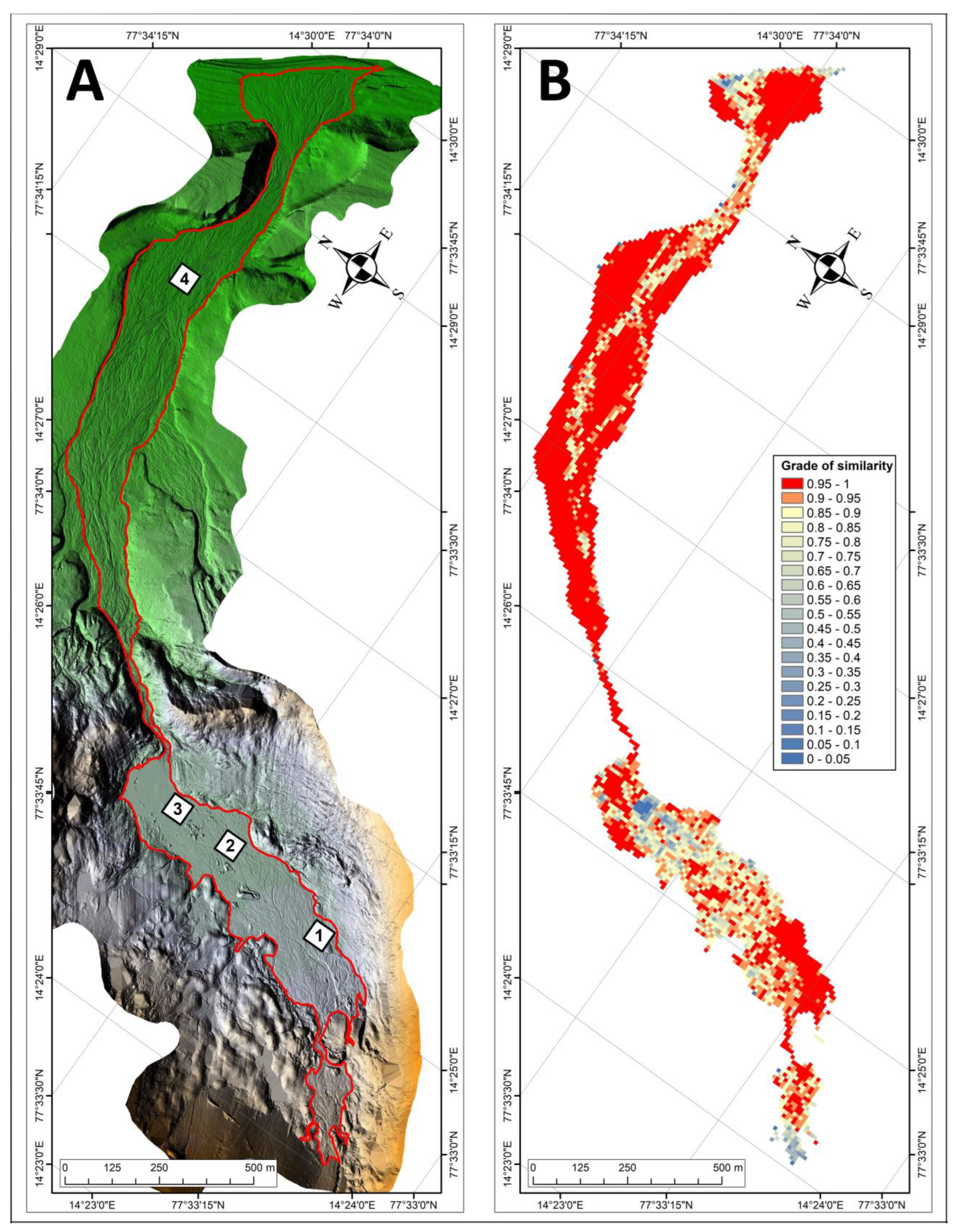
3.2. Relief Similarity and Change Detection
4. Discussion
5. Conclusions
Author Contributions
Funding
Data Availability Statement
Acknowledgments
Conflicts of Interest
References
- Snow, Water, Ice and Permafrost in the Arctic (SWIPA): Climate Change and the Cryosphere; AMAP: Oslo, Norway, 2011; ISBN 978-82-7971-071-4.
- Amélineau, F.; Grémillet, D.; Harding, A.M.A.; Walkusz, W.; Choquet, R.; Fort, J. Arctic Climate Change and Pollution Impact Little Auk Foraging and Fitness across a Decade. Sci. Rep. 2019, 9, 1014. [Google Scholar] [CrossRef]
- Vaughan, D.G.; Comiso, J.C.; Allison, I.; Carrasco, J.; Kaser, G.; Kwok, R.; Mote, P.; Murray, T.; Paul, F.; Ren, J.; et al. Observations: Cryosphere. Clim. Chang. 2013, 2103, 317–382. [Google Scholar]
- Kääb, A.; Berthier, E.; Nuth, C.; Gardelle, J.; Arnaud, Y. Contrasting Patterns of Early Twenty-First-Century Glacier Mass Change in the Himalayas. Nature 2012, 488, 495–498. [Google Scholar] [CrossRef]
- Woul, M.D.; Hock, R. Static Mass-Balance Sensitivity of Arctic Glaciers and Ice Caps Using a Degree-Day Approach. Ann. Glaciol. 2005, 42, 217–224. [Google Scholar] [CrossRef]
- Arheimer, B.; Lindström, G. Climate Impact on Floods: Changes in High Flows in Sweden in the Past and the Future (1911–2100). Hydrol. Earth Syst. Sci. 2015, 19, 771–784. [Google Scholar] [CrossRef]
- Kociuba, W.; Gajek, G.; Franczak, Ł. A Short-Time Repeat TLS Survey to Estimate Rates of Glacier Retreat and Patterns of Forefield Development (Case Study: Scottbreen, SW Svalbard). Resources 2020, 10, 2. [Google Scholar] [CrossRef]
- Ashworth, P.J.; Ferguson, R.I. Interrelationships of Channel Processes, Changes and Sediments in a Proglacial Braided River. Geogr. Ann. Ser. A Phys. Geogr. 1986, 68, 361–371. [Google Scholar] [CrossRef]
- Ashworth, P.J.; Best, J.L.; Jones, M. Relationship between Sediment Supply and Avulsion Frequency in Braided Rivers. Geology 2004, 32, 21. [Google Scholar] [CrossRef]
- Carrivick, J.L.; Geilhausen, M.; Warburton, J.; Dickson, N.E.; Carver, S.J.; Evans, A.J.; Brown, L.E. Contemporary Geomorphological Activity throughout the Proglacial Area of an Alpine Catchment. Geomorphology 2013, 188, 83–95. [Google Scholar] [CrossRef]
- Beylich, A.A.; Laute, K. Sediment Sources, Spatiotemporal Variability and Rates of Fluvial Bedload Transport in Glacier-Connected Steep Mountain Valleys in Western Norway (Erdalen and Bødalen Drainage Basins). Geomorphology 2015, 228, 552–567. [Google Scholar] [CrossRef]
- Ashworth, P.J.; Best, J.L.; Jones, M.A. The Relationship between Channel Avulsion, Flow Occupancy and Aggradation in Braided Rivers: Insights from an Experimental Model. Sedimentology 2007, 54, 497–513. [Google Scholar] [CrossRef]
- Kociuba, W. Assessment of Sediment Sources throughout the Proglacial Area of a Small Arctic Catchment Based on High-Resolution Digital Elevation Models. Geomorphology 2017, 287, 73–89. [Google Scholar] [CrossRef]
- Kociuba, W.; Krząstek, P.; Superson, J. Combining GPS-RTK and rephotographic methodolo-gies for the assessment of transformations of the ephemeral landforms of the near foreland of a valley glacier (Scottbreen, Svalbard). Z. Geomorphol. 2016, 60, 29–44. [Google Scholar] [CrossRef]
- Chandler, B.M.P.; Lovell, H.; Boston, C.M.; Lukas, S.; Barr, I.D.; Benediktsson, Í.Ö.; Benn, D.I.; Clark, C.D.; Darvill, C.M.; Evans, D.J.A.; et al. Glacial Geomorphological Mapping: A Review of Approaches and Frameworks for Best Practice. Earth-Sci. Rev. 2018, 185, 806–846. [Google Scholar] [CrossRef]
- Kääb, A.; Lefauconnier, B.; Melvold, K. Flow field of Kronebreen, Svalbard, using repeated Landsat 7 and ASTER data. Ann. Glaciol. 2005, 42, 7–13. [Google Scholar] [CrossRef]
- Brasington, J.; Rumsby, B.T.; McVey, R.A. Monitoring and Modelling Morphological Change in a Braided Gravel-Bed River Using High Resolution GPS-Based Survey. Earth Surf. Process. Landf. 2000, 25, 973–990. [Google Scholar] [CrossRef]
- Charlton, M.E.; Large, A.R.G.; Fuller, I.C. Application of Airborne LiDAR in River Environments: The River Coquet, Northumberland, UK. Earth Surf. Process. Landf. 2003, 28, 299–306. [Google Scholar] [CrossRef]
- Bamber, J.L.; Krabill, W.; Raper, V.; Dowdeswell, J.A.; Oerlemans, J. Elevation Changes Measured on Svalbard Glaciers and Ice Caps from Airborne Laser Data. Ann. Glaciol. 2005, 42, 202–208. [Google Scholar] [CrossRef]
- Arnold, N.S.; Rees, W.G.; Devereux, B.J.; Amable, G.S. Evaluating the Potential of High-resolution Airborne LiDAR Data in Glaciology. Int. J. Remote Sens. 2006, 27, 1233–1251. [Google Scholar] [CrossRef]
- Glenn, N.F.; Streutker, D.R.; Chadwick, D.J.; Thackray, G.D.; Dorsch, S.J. Analysis of LiDAR-Derived Topographic Information for Characterizing and Differentiating Landslide Morphology and Activity. Geomorphology 2006, 73, 131–148. [Google Scholar] [CrossRef]
- Heritage, G.L.; Milan, D.J.; Large, A.R.G.; Fuller, I.C. Influence of Survey Strategy and Interpolation Model on DEM Quality. Geomorphology 2009, 112, 334–344. [Google Scholar] [CrossRef]
- Kociuba, W.; Kubisz, W.; Zagórski, P. Use of Terrestrial Laser Scanning (TLS) for Monitoring and Modelling of Geomorphic Processes and Phenomena at a Small and Medium Spatial Scale in Polar Environment (Scott River—Spitsbergen). Geomorphology 2014, 212, 84–96. [Google Scholar] [CrossRef]
- Bangen, S.G.; Wheaton, J.M.; Bouwes, N.; Bouwes, B.; Jordan, C. A Methodological Intercomparison of Topographic Survey Techniques for Characterizing Wadeable Streams and Rivers. Geomorphology 2014, 206, 343–361. [Google Scholar] [CrossRef]
- Stepinski, T.F.; Jasiewicz, J. Geomorphons—A New Approach to Classification of Landforms. Proc. Geomorphometry. 2011, pp. 109–112. Available online: https://geomorphometry.org/wp-content/uploads/2021/07/StepinskiJasiewicz2011geomorphometry.pdf (accessed on 16 October 2023).
- Jasiewicz, J.; Stepinski, T.F. Geomorphons—A Pattern Recognition Approach to Classification and Mapping of Landforms. Geomorphology 2013, 182, 147–156. [Google Scholar] [CrossRef]
- Dąbrowski, A.; Jasiewicz, J. Zastosowanie Form Morfometrycznych Do Analizy Zróżnicowania Wybranych Typów Powierzchni na Obszarach Młodoglacjalnych. Badania fizjograficzne 2014, R. V seria A, 095-111, Poznańskie Towarzystwo Przyjaciół Nauk oraz Wydziału Nauk Geograficznych i Geologicznych i Wydziału Biologii Uniwersytetu im. Adama Mickiewicza w Poznaniu, Poznań, Poland. Available online: https://repozytorium.amu.edu.pl/server/api/core/bitstreams/1c6c790e-5d86-4f5f-865b-f91c04f9c35d/content (accessed on 19 October 2023).
- Jasiewicz, J.; Netzel, P.; Stepinski, T.F. Landscape Similarity, Retrieval, and Machine Mapping of Physiographic Units. Geomorphology 2014, 221, 104–112. [Google Scholar] [CrossRef]
- Gawrysiak, L. Segmentacje Rzeźby Terenu z Wykorzystaniem Metod Automatycznej Klasyfikacji i ich Relacja do Mapy Geomorfologicznej; MCSU Press: Lublin, Poland, 2018. [Google Scholar]
- Gawrysiak, L.; Kociuba, W. Application of Geomorphons for Analysing Changes in the Morphology of a Proglacial Valley (Case Study: The Scott River, SW Svalbard). Geomorphology 2020, 371, 107449. [Google Scholar] [CrossRef]
- Bartoszewski, S.; Gluza, A.; Siwek, K.; Zagórski, P. Temperature and Rainfall Control of Outflow from the Scott Glacier Catchment (Svalbard) in the Summers of 2005 and 2006. Nor. Geogr. Tidsskr.-Nor. J. Geogr. 2009, 63, 107–114. [Google Scholar] [CrossRef]
- Harasimiuk, M.; Gajek, G. Tectonic and lithology. In Geographical Environment of NW Part of Wedel Jarlsberg Land (Spitsbergen, Svalbard); Zagórski, P., Harasimiuk, M., Rodzik, J., Eds.; MCSU Press: Lublin, Poland, 2013; pp. 34–47. [Google Scholar]
- Leica-Geosystems. Leica ScanStation C10—Datasheet. 2012. Available online: https://www.geooptic.ru/static/files/leica-scanstation-c10-ds.pdf (accessed on 30 August 2023).
- Smith, M.W.; Vericat, D. Evaluating Shallow-Water Bathymetry from Through-Water Terrestrial Laser Scanning Under a Range of Hydraulic and Physical Water Quality Conditions. River Res. Apps 2014, 30, 905–924. [Google Scholar] [CrossRef]
- Zhang, W.; Qi, J.; Wan, P.; Wang, H.; Xie, D.; Wang, X.; Yan, G. An Easy-to-Use Airborne LiDAR Data Filtering Method Based on Cloth Simulation. Remote Sens. 2016, 8, 501. [Google Scholar] [CrossRef]
- Netzel, P.; Nowosad, J.; Jasiewicz, J.; Niesterowicz, J.; Stepinski, T. Geopat 2: User’s Manual. 2018, 521. Available online: https://zenodo.org/records/1291123/files/GeoPAT2_Manual.pdf?download=1 (accessed on 19 October 2023).
- Haralick, R.M.; Shanmugam, K.; Dinstein, I. Textural Features for Image Classification. IEEE Trans. Syst. Man. Cybern. 1973, SMC-3, 610–621. [Google Scholar] [CrossRef]
- Lin, J. Divergence Measures Based on the Shannon Entropy. IEEE Trans. Inform. Theory 1991, 37, 145–151. [Google Scholar] [CrossRef]
- Gogołek, W.; Lewandowski, W. Preliminary geomorphological characteristic of Linnedalen (Spitsbergen, Svalbard Archipelago). Pol. Polar Res. 1980, 1, 7–19. [Google Scholar]
- Lacika, J.; Musiał, A. Relief-forming processes in the polar zone. Example from Nordenskiold Land (West Spitsbergen). Misc. Geogr 1988, 3, 69–78. [Google Scholar] [CrossRef]
- Ewertowski, M.W.; Evans, D.J.A.; Robertsaand, D.H.; Tomczyk, A.M. Glacial geomorphology of the terrestrial margins of the tidewater glacier, Nordenskiöldbreen, Svalbard. J. Maps 2016, 12, 476–487. [Google Scholar] [CrossRef]
- Tomczyk, A.; Ewertowski, M.W. Surface morphological types and spatial distribution of fan-shaped landforms in the periglacial high-Arctic environment of central Spitsbergen, Svalbard. J. Maps 2017, 13, 239–251. [Google Scholar] [CrossRef]
- Jania, J.; Szczypek, T. Geomorphological mapping of the Hornsund fjord region from interpretation of aerial photographs. Fotointerpret. W Geogr. 1987, 19, 9108–9128. [Google Scholar]
- Szczęsny, R. Quaternary landforms and deposits in southern Spitsbergen on the ground of photointerpretation. Pol. Polar Res. 1991, 12, 289–343. [Google Scholar]
- Karczewski, A.; Andrzejewski, L.; Chmal, H.; Jania, J.; Kłysz, P.; Kostrzewski, A.; Lindner, L.; Marks, L.; Pękala, K.; Pulina, M.; et al. Hornsund, Spitsbergen. Geomorphology. 1:75 000 (Map); Silesian University: Katowice, Poland, 1984. [Google Scholar]
- Allaart, L.; Schomacker, A.; Håkansson, L.M.; Farnsworth, W.R.; Brynjólfsson, S.; Grumstad, A.; Kjellman, S.E. Geomorphology and surficial geology of the Femmilsjøen area, northern Spitsbergen. Geomorphology 2021, 382, 107693. [Google Scholar] [CrossRef]
- Ewertowski, M.W.; Tomczyk, A.M.; Evans, D.J.A.; Roberts, D.H.; Ewertowski, W. Operational Framework for Rapid, Very-High Resolution Mapping of Glacial Geomorphology Using Low-Cost Unmanned Aerial Vehicles and Structure-from-Motion Approach. Remote Sens. 2019, 11, 65. [Google Scholar] [CrossRef]
- Woźniak, P. High Resolution Elevation Data in Poland. In Geomorphometry for Geosciences; Adam Mickiewicz Uniwersity: Poznań, Poland, 2015; pp. 13–14. [Google Scholar]
- Gawrysiak, L.; Kociuba, W. LiDAR-Derived Relief Typology of Loess Patches (East Poland). Remote Sens. 2023, 15, 1875. [Google Scholar] [CrossRef]
- Rodzik, J.; Gajek, G.; Reder, J.; Zagórski, P. Glacial geomorphology. In Geographical Environment of NW Part of Wedel Jarlsberg Land (Spitsbergen, Svalbard); Zagórski, P., Harasimiuk, M., Rodzik, J., Eds.; MCSU Press: Lublin, Poland, 2013; pp. 36–165. [Google Scholar]
- Carrivick, J.L.; Berry, K.; Geilhausen, M.; James, W.H.M.; Williams, C.; Brown, L.E.; Rippin, D.M.; Carver, S.J. Decadal-scale Changes of the Ödenwinkelkees, Central Austria, Suggest Increasing Control of Topography and Evolution towards Steady State. Geogr. Ann. Ser. A Phys. Geogr. 2015, 97, 543–562. [Google Scholar] [CrossRef]
- Kociuba, W.; Janicki, G.; Dyer, J.L. Contemporary Changes of the Channel Pattern and Braided Gravel-Bed Floodplain under Rapid Small Valley Glacier Recession (Scott River Catchment, Spitsbergen). Geomorphology 2019, 328, 79–92. [Google Scholar] [CrossRef]
- Marren, P.M. Magnitude and Frequency in Proglacial Rivers: A Geomorphological and Sedimentological Perspective. Earth-Sci. Rev. 2005, 70, 203–251. [Google Scholar] [CrossRef]
- Marren, P.M.; Toomath, S.C. Channel Pattern of Proglacial Rivers: Topographic Forcing Due to Glacier Retreat. Earth Surf. Process. Landf. 2014, 39, 943–951. [Google Scholar] [CrossRef]
- Owczarek, P.; Nawrot, A.; Migała, K.; Malik, I.; Korabiewski, B. Flood-plain Responses to Contemporary Climate Change in Small H Igh-A Rctic Basins (S Valbard, N Orway). Boreas 2014, 43, 384–402. [Google Scholar] [CrossRef]
- Cossart, É. Landform Connectivity and Waves of Negative Feedbacksduring the Paraglacial Period, a Case Study: The Tabuc Subcatchment since the End of the Little Ice Age (Massif Des Écrins, France). Geomorphologie 2008, 14, 249–260. [Google Scholar] [CrossRef]
- Kociuba, W.; Janicki, G. Changeability of Movable Bed-surface Particles in Natural, Gravel-bed Channels and Its Relation to Bedload Grain Size Distribution (Scott River, Svalbard). Geogr. Ann. Ser. A Phys. Geogr. 2015, 97, 507–521. [Google Scholar] [CrossRef]
- Kociuba, W. Geomorphic Changes of the Scott River Alluvial Fan in Relation to a Four-Day Flood Event. Water 2023, 15, 1368. [Google Scholar] [CrossRef]
- Lehmann-Konera, S.; Kociuba, W.; Chmiel, S.; Franczak, Ł.; Polkowska, Ż. Effects of Biotransport and Hydro-Meteorological Conditions on Transport of Trace Elements in the Scott River (Bellsund, Spitsbergen). PeerJ 2021, 9, e11477. [Google Scholar] [CrossRef]


| Group | n * | Area (ha) | Area (%) | Min | Max | Mean | Standard Deviation |
|---|---|---|---|---|---|---|---|
| 1 | 85 | 7.70 | 18.55 | 0.003 | 0.657 | 0.125 | 0.086 |
| 2 | 16 | 1.14 | 2.75 | 0.017 | 0.459 | 0.192 | 0.099 |
| 3 | 40 | 1.48 | 3.57 | 0.008 | 0.374 | 0.125 | 0.070 |
| 4 | 62 | 29.49 | 71.04 | 0.003 | 0.541 | 0.122 | 0.077 |
| 5 | 6 | 1.55 | 3.73 | 0.006 | 0.183 | 0.093 | 0.066 |
| 6 | 4 | 0.15 | 0.36 | 0.004 | 0.142 | 0.073 | 0.061 |
| Total | 213 | 41.51 | 100.00 | 0.003 | 1.000 | 0.283 | 0.226 |
| Group | n * | Area (ha) | Area (%) | Min | Max | Mean | Standard Deviation |
|---|---|---|---|---|---|---|---|
| 1 | 57 | 2.11 | 5.08 | 0.006 | 0.433 | 0.129 | 0.073 |
| 2 | 73 | 36.29 | 87.42 | 0.001 | 0.569 | 0.111 | 0.079 |
| 3 | 12 | 1.97 | 4.75 | 0.007 | 0.674 | 0.200 | 0.161 |
| 4 | 18 | 0.90 | 2.17 | 0.025 | 0.500 | 0.168 | 0.090 |
| 5 | 15 | 0.24 | 0.58 | 0.009 | 0.421 | 0.170 | 0.111 |
| Total | 175 | 41.51 | 100.00 | 0.002 | 0.288 | 0.998 | 0.236 |
| Range Number | Range | n * | % (Area) | Area (ha) |
|---|---|---|---|---|
| 1 | 0.00–0.05 | 7 | 0.17 | 0.07 |
| 2 | 0.05–0.10 | 3 | 0.07 | 0.03 |
| 3 | 0.10–0.15 | 3 | 0.07 | 0.03 |
| 4 | 0.15–0.20 | 4 | 0.10 | 0.04 |
| 5 | 0.20–0.25 | 3 | 0.07 | 0.03 |
| 6 | 0.25–0.30 | 15 | 0.36 | 0.15 |
| 7 | 0.30–0.35 | 14 | 0.34 | 0.14 |
| 8 | 0.35–0.40 | 6 | 0.14 | 0.06 |
| 9 | 0.40–0.45 | 15 | 0.36 | 0.15 |
| 10 | 0.45–0.50 | 22 | 0.53 | 0.22 |
| 11 | 0.50–0.55 | 28 | 0.68 | 0.28 |
| 12 | 0.55–0.60 | 44 | 1.06 | 0.44 |
| 13 | 0.60–0.65 | 36 | 0.87 | 0.36 |
| 14 | 0.65–0.70 | 80 | 1.93 | 0.80 |
| 15 | 0.70–0.75 | 113 | 2.73 | 1.13 |
| 16 | 0.75–0.80 | 136 | 3.28 | 1.36 |
| 17 | 0.80–0.85 | 215 | 5.19 | 2.15 |
| 18 | 0.85–0.90 | 400 | 9.65 | 4.00 |
| 19 | 0.90–0.95 | 713 | 17.20 | 7.13 |
| 20 | 0.95–1.00 | 2,289 | 55.20 | 22.89 |
| Total | 4,162 | 100.00 | 41.62 |
Disclaimer/Publisher’s Note: The statements, opinions and data contained in all publications are solely those of the individual author(s) and contributor(s) and not of MDPI and/or the editor(s). MDPI and/or the editor(s) disclaim responsibility for any injury to people or property resulting from any ideas, methods, instructions or products referred to in the content. |
© 2023 by the authors. Licensee MDPI, Basel, Switzerland. This article is an open access article distributed under the terms and conditions of the Creative Commons Attribution (CC BY) license (https://creativecommons.org/licenses/by/4.0/).
Share and Cite
Gawrysiak, L.; Kociuba, W. Similarity and Change Detection of Relief in a Proglacial River Valley (Scott River, SW Svalbard). Remote Sens. 2023, 15, 5066. https://doi.org/10.3390/rs15205066
Gawrysiak L, Kociuba W. Similarity and Change Detection of Relief in a Proglacial River Valley (Scott River, SW Svalbard). Remote Sensing. 2023; 15(20):5066. https://doi.org/10.3390/rs15205066
Chicago/Turabian StyleGawrysiak, Leszek, and Waldemar Kociuba. 2023. "Similarity and Change Detection of Relief in a Proglacial River Valley (Scott River, SW Svalbard)" Remote Sensing 15, no. 20: 5066. https://doi.org/10.3390/rs15205066