1. Introduction
The ionosphere, situated between 60 and 2000 km above the Earth’s surface, plays a vital role in electromagnetic wave propagation, influenced by solar-radiation-induced ionization [
1]. The speed at which the transmitted electromagnetic signals from the GNSS (global navigation satellite system) satellites propagate through the ionosphere depends on the electron density along the line of sight between the satellite and the receiver. Upon traversing the ionosphere, GNSS signals may encounter two distinct forms of perturbations: Firstly, the introduction of an error in the estimated range due to the signal’s delay that is proportional to the integrated electron density (slant total electron content—sTEC), and secondly, the occurrence of signal characteristic fluctuations resulting from irregularities in the ionosphere’s electron density distribution [
2].
The use of GNSS signals, renowned for their global availability and signal propagation characteristics, has been widely investigated and exploited as a powerful tool for ionospheric studies across diverse spatial and temporal scales. Ground-based atmospheric-sounding techniques employing continuously operating reference station (CORS) networks and GNSS receivers, which operate on low Earth orbit (LEO) satellites for the analysis of refracted radio signals via GNSS radio occultation (GNSS-RO), provide key observations for improving global weather forecasts [
3]. To further broaden the observations, GNSS reflectometry (GNSS-R) has emerged as a complementary technique that leverages signals reflected off the Earth’s surface. This approach not only facilitates the retrieval of reflecting surface properties but also serves as an atmospheric-sounding tool.
In order to understand ionospheric ranging delays within space-borne GNSS-R, simulations are conducted as detailed in [
4]. The simulation is based on the Cyclone GNSS (CYGNSS) [
5] mission and encompasses different elevation angles, latitudes, and solar activities. The results reveal an inverse relationship between the satellite elevation angle and ionospheric delay, with a larger ionospheric influence at low latitudes. In [
6], the impact of scintillation effects on reflectometry has been explored using data from UK TechDemoSat-1 [
7]. These effects lead to a degradation of the signal-to-noise ratio that can be utilized for altimetry and scatterometry performance assessments. More recently, studies have been carried out to retrieve the total electron content (TEC) from coherent reflectometry observations. In the work presented in [
8], a methodology was introduced for sTEC estimation along the paths of incident and reflected signal rays. This estimation is based on coherent dual-frequency GNSS-R measurements obtained from Spire Global low Earth orbit (LEO) CubeSats. The outcomes have demonstrated a favorable alignment between reflectometry sTEC estimations and the global ionospheric TEC maps (GIM). Furthermore, an algorithm outlined in [
9] combines sTEC observation from space-borne reflectometry using CubeSats and data collected from ground-based GNSS stations to generate vertical TEC (vTEC) maps in the Arctic region. Simulations conducted within this study under diverse conditions, involving variations in temporal resolution, solar activity levels, and the number of reflection events, have demonstrated enhanced accuracy in vTEC estimations when coherent GNSS-R observations are incorporated.
In the domain of GNSS-R, it has been empirically established that coherent observations are more frequently observed in the presence of smooth reflecting surfaces, such as sea ice, regions with low sea states, or inland waters, and at low grazing angles [
10,
11,
12]. Nonetheless, within this range of elevation angles, it is important to note that the trajectories of the LEO GNSS-R rays entail a longer path through the ionosphere. This extended path results in a more pronounced ionospheric impact on the signals themselves. The representation (not to scale) of the LEO GNSS-R configuration along the grazing angle rays’ paths and its interaction with the ionosphere are illustrated in
Figure 1.
As described in [
13], dual-frequency receivers possess the capability to mitigate these first-order ionospheric effects through the utilization of a linear combination (ionosphere-free) of either code or carrier measurements. Conversely, single-frequency receivers must rely on applying a model to correct for ionospheric refraction, which can introduce delays of several tens of meters. For the Galileo GNSS constellation, the European GNSS Open Service has adopted the Neustrelitz Total Electron Content Model NTCM [
14] (NTCM-G) or NeQuick 2 [
15] (NeQuick-G) models to provide real-time ionospheric corrections for single-frequency receivers [
16].
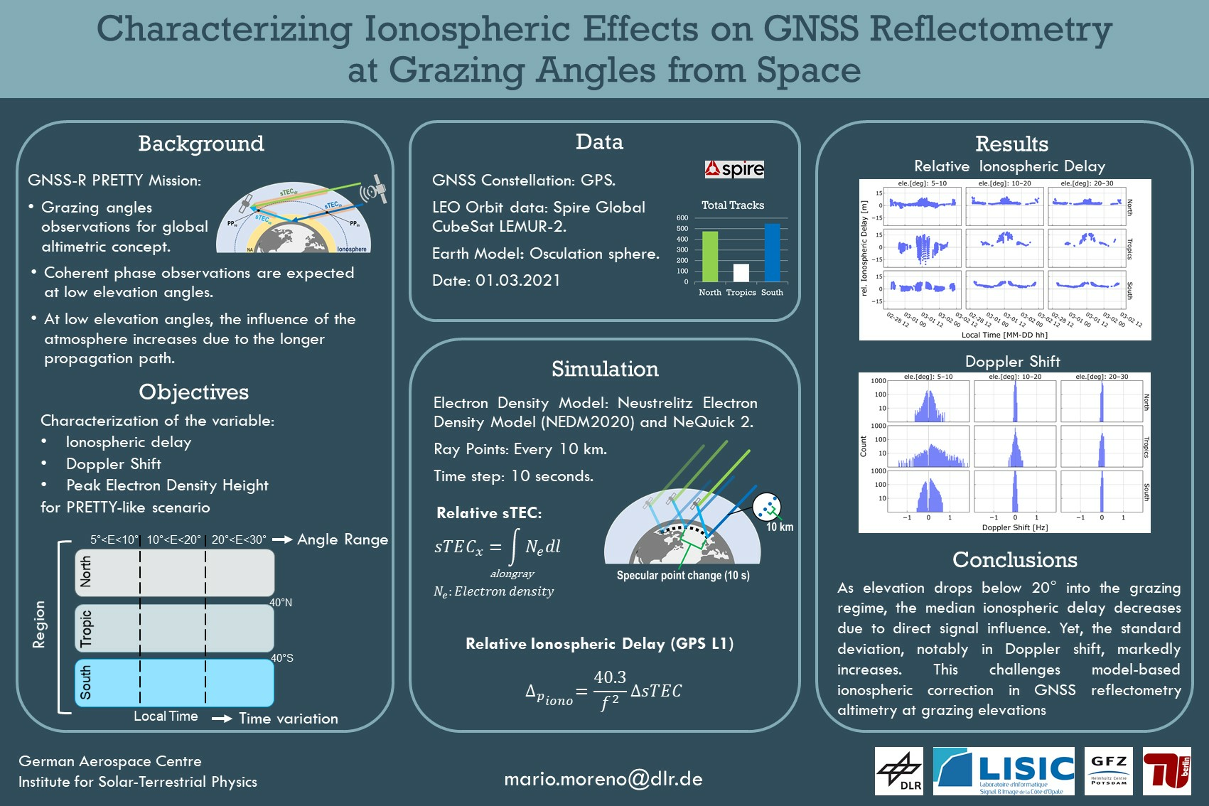
This study is in preparation for the European Space Agency’s GNSS-R CubeSat mission “PRETTY” (passive reflectometry and dosimetry) [
17]. The mission’s primary goal is to retrieve sea surface height using grazing angle observations. Since PRETTY operates at a single frequency (L5), it requires model-based ionospheric corrections. This study provides a comprehensive characterization of ionospheric effects, at the grazing angle range (5°–30°), considering satellite geometry, latitude-dependent regions, temporal variations, and solar activity. It analyzes variability in the ionospheric group delay, Doppler shift, and peak electron density height. Additionally, the uncertainty in model-based ionospheric corrections for GNSS-R group delay altimetry is assessed.
The analysis is based on utilizing the sTEC obtained from three-dimensional, time-dependent models. To assess model uncertainty, the sTEC values computed using the Neustrelitz Electron Density Model (NEDM2020) [
18] are used as a reference and compared with the sTEC retrievals from NeQuick 2. Simulations are conducted to replicate conditions similar to those of the PRETTY mission, utilizing orbit data from the GNSS-R Spire Global Lemur-2 constellation. To provide a comprehensive analysis, the results are categorized into three elevation angle ranges: very-low (5°–10°), low (10°–20°), and mid-low (20°–30°). These categories are further grouped by latitude into three distinct regions: north, tropics, and south. Additionally, this study considers variations in local time and solar activity. Low solar activity (LSA) is represented by F10.7 = 75 in March 2021 and high solar activity (HSA) by F10.7 = 180 in March 2023.
The structure of this paper is outlined as follows:
Section 2 presents the GNSS-R data descriptions, reflection events, and ray point settings for the simulations.
Section 3 illustrates the methodologies utilized for the determination of parameters such as sTEC, relative ionospheric delay, Doppler shift, and ionospheric piercing points. Subsequently,
Section 4 presents the results and analysis of the parameters explained in
Section 3. Finally, in
Section 5, a discussion of the findings is presented along with the conclusions in
Section 6.
2. GNSS-R Data and Reflection Events
2.1. LEO Data
The LEO data used in this study consist of a total of 1188 reflection events on 1 March 2021, sourced from Spire Global Inc. Currently, the Spire Lemur-2 constellation comprises more than 80 GNSS radio occultation CubeSats, out of which about 30 have been adapted to acquire GNSS reflectometry measurements at grazing angles [
19]. The Lemur-2 satellites follow a Sun-synchronous orbit, with altitudes ranging from 400 to 600 km and varying orbit inclinations. This orbital configuration enables them to conduct GNSS-R measurements, encompassing all latitudes of the Earth.
The Spire grazing angle GNSS-R products are collected with a focus on specific regions, including the polar areas, the Gulf of Mexico, and southeast Asia. These regions are selected due to their favorable characteristics, such as sea ice surfaces and calm ocean surfaces, which enable the best performance of coherent reflectometry measurements [
10].
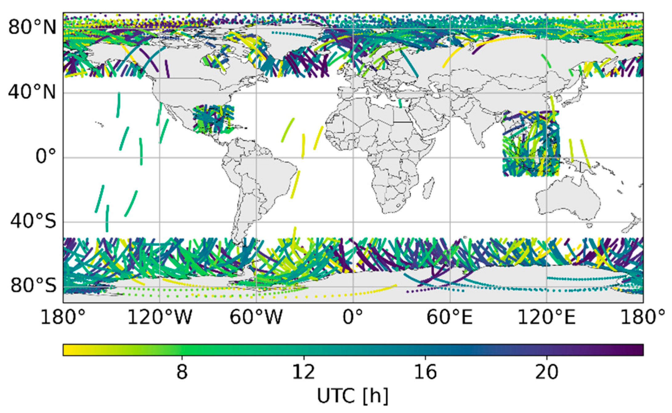
Figure 2 displays the track positions of the specular points distributed across both polar regions, as well as in the mid-latitude and tropical regions at different local times. Given the geographical distribution of the events, the dataset has been categorized into three distinct regions: north, covering latitudes between 40°N and 90°N; tropics, spanning latitudes between 40°N and 40°S; and south, covering latitudes between 40°S and 90°S.
Each Lemur-2 satellite event lasts an average of 4 min, resulting in a total of about 80 h of recorded data. The recording durations vary, with a minimum of 1 min and a maximum of 6 min.
Table 1 shows the number of events per region (north, tropics, and south) along with their corresponding durations in minutes.
A total of 21 CubeSats from the Spire constellation are evaluated. The metadata include the space vehicle number (SVN) of the Lemur-2 satellite, as well as information about the GNSS satellite and constellation from which the CubeSat receives the reflected signals. For the simulation in this study, the GNSS constellation employed is GPS (global positioning system). Upon analyzing the Spire data, it is found that each Lemur-2 satellite receives the reflected signal from 4 to 19 GPS satellites during different time windows, depending on the positions of the transmitters and the receiver. The Spire SVN and GPS pseudo-random noise code (PRN) are presented in
Table 2.
2.2. Specular Point Positions and Ray Points
The specular point positions and the ray tracing of the direct, incident, and reflected signals are calculated based on the methodology presented in [
11,
20]. A geometrical model is employed to characterize specular reflections and determine the specular point position, considering the Earth’s surface curvature. For this model, the transmitter
and receiver
positions are needed in an Earth-centered Earth-fixed (ECEF) frame. The
position is extracted from the Spire data files. To obtain this position, the Lemur-2 satellites are equipped with a zenith dual-frequency (L1 and L2) antenna, which facilitates precise orbit determination (POD). The
position is derived from the broadcasted GPS ephemeris. The Earth’s curvature is modeled with an osculating spherical surface with respect to the WGS-84 ellipsoid at a reference specular point. An iterative solution is employed to find the best-fitting sphere that satisfies the condition of equal incident and reflected angles (specular reflection) [
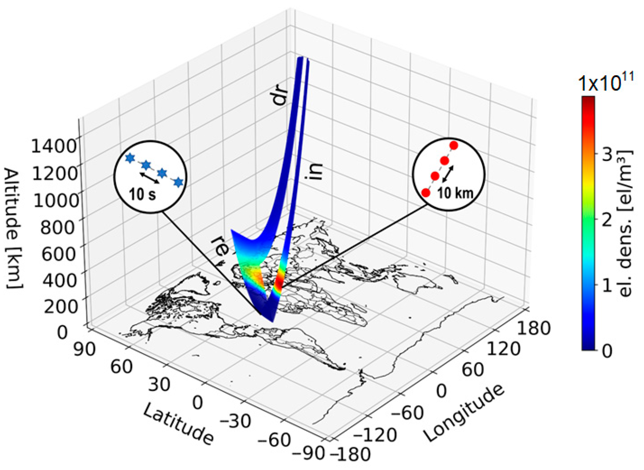
20]. The specular point positions are calculated at 10 s intervals on the receiver trajectory. A ray-tracing module is set to compute ray points every 10 km along the three ray paths:
to
(incident),
to
(reflected), and
to
(direct). The positions of the ray points (latitude, longitude, and ellipsoidal height) are subsequently utilized to obtain the electron density from the ionospheric electron density models.
Figure 3 illustrates an example of the electron density retrieval from the NEDM2020 model depicting the change along the specular point tracks every 10 s (blue stars), and the ray points change every 10 km (red dots) along the incident (in), reflected (re), and direct (dr) ray paths.
Following the ray tracing, a total of 28,790 reflection events are obtained. The total number of reflection events by region is depicted in
Figure 4a. Additionally,
Figure 4b illustrates the distribution of reflection events concerning the elevation angle by region. Notably, the south pole region exhibits a higher number of events; however, all regions show similar behavior, with a higher concentration of events in the elevation range between 5° and 20°.
3. Methodology
3.1. Electron Density Models
The electron density in this study is obtained from two three-dimensional and time-dependent electron density models: the Neustrelitz Electron Density Model (NEDM2020) [
18] and the NeQuick 2 model [
15]. For both models, the input values depending on solar activity are the solar radio flux index F10.7, month, geographic latitude and longitude, height, and universal time (UT). The output obtained is the electron concentration at the specified location and time.
The NeQuick 2 model was developed at the Aeronomy and Radiopropagation Laboratory of The Abdus Salam International Centre for Theoretical Physics (ICTP), Trieste, Italy, and at the Institute for Geophysics, Astrophysics, and Meteorology (IGAM) of the University of Graz, Austria. This model comprises vertical profiles consisting of multiple Epstein layers, and it derives essential electron peak density and height parameters through spatial and temporal interpolation from a comprehensive set of global maps. Consequently, NeQuick 2 incurs significant computational demands in terms of time and processing power [
14].
On the other hand, the NEDM2020 model was developed at the German Aerospace Center in the Institute for Solar–Terrestrial Physics (DLR-SO), Neustrelitz, Germany. Including the NTCM model, this model relies on about 100 model coefficients and a set of empirically fixed parameters. Remarkably, the electron density values can be directly computed for any specified location and time without the requirement for the specialized temporal or spatial interpolation of parameters, making it faster than the NeQuick 2 model in terms of computational efficiency [
21].
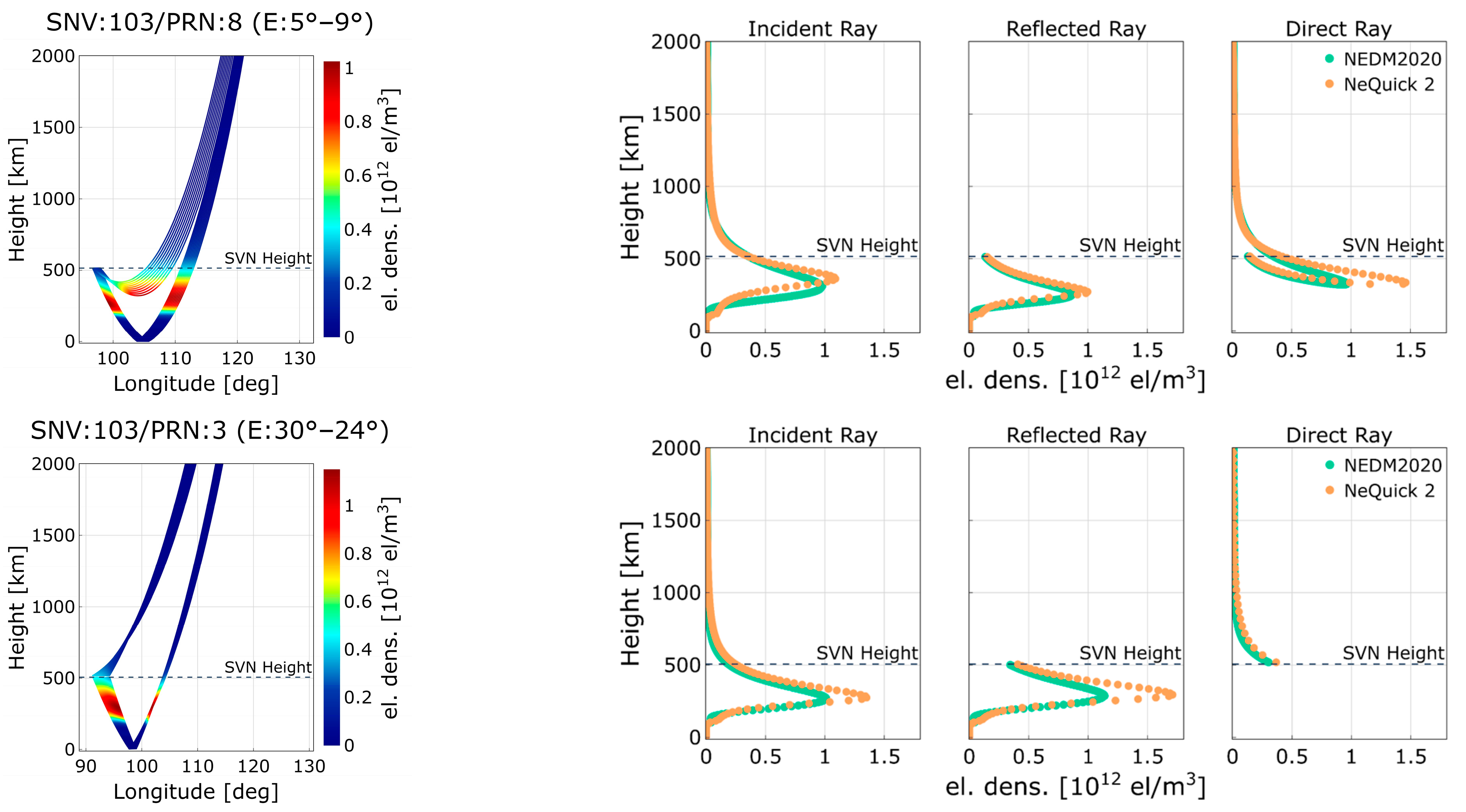
A model comparison of electron density profiles is presented in
Figure 5 featuring one example at very low (first row) and mid-low (second row) elevation angle events. The first column displays the electron density per ray mapped along the specular point change using the NEDM2020 model. The subsequent columns (second, third, and fourth) illustrate the electron density profile comparison between the NEDM2020 and NeQuick 2 models for the incident, reflected, and direct rays, respectively.
3.2. Ionospheric Group Delay Computation
The GNSS electromagnetic signal propagation speed in the ionosphere depends on electron density
, which is influenced by daytime ionization and nighttime recombination processes. According to [
13], when considering the signal code measurements, the difference between the measured range (using a signal of frequency
in
) and the Euclidean distance between the satellite and receiver is expressed as follows:
is the term used for the group ionospheric refraction, and the integral is known as the slant total electron content
, representing the numerical integration of the electron density along the ray path.
corresponds to the GNSS signal frequency, and in this study, the GPS L1 frequency is
. The
is computed for each ray, including the incident
, reflected
, and direct
rays, respectively. The
is expressed in total electron content units (TECUs) where one TECU corresponds to
electrons per square meter
. Finally, the group ionospheric delay in meters (for each ray) is obtained from:
As presented in [
22], the relative delay between the direct and reflected signals is denoted as
where
is the cumulative path of the incident and reflected rays, while
corresponds to the direct path. The relative delay can be influenced by various contributing factors, such as the standard sources of delay within the GNSS signals. Therefore, the extended version of
can be written as:
where
represents the relative geometrical delay, and
and
correspond to the relative tropospheric and ionospheric delays, respectively.
is a bias induced by the surface roughness. The instrumental error is denoted by
, and
represents unmodeled errors.
GNSS-R Group Delay Altimetry and Ionospheric Delay Uncertainty
Based on the analysis conducted in [
23], the ionospheric delay constitutes a significant component within the error budget associated with GNSS-R ocean surface altimetry retrievals. At elevation angles above 60°, the uncorrected ionospheric delay can reach ~15 m during daytime and ~7 at nighttime. The ionospheric group delay bias propagates to an altimetric bias based on the relation between the height offset
and the signal path
. Consequently, when considering only the ionospheric altimetric error, where
is the elevation angle, it can be expressed as:
Assuming a relative uncertainty of 30% for the ionospheric delay bias, as established in [
20], we introduce normally distributed random errors with a respective standard deviation
).
3.3. Doppler Shift Computation
The Doppler shift of a GNSS signal is predominantly influenced by the relative velocity between the transmitter satellite and the receiver, along with a common offset that is proportional to the error in the receiver clock’s frequency. However, as demonstrated in [
24,
25], various ionospheric effects, such as changes in the redistribution and density of electrons in the ionosphere, lead to frequency variations in the electromagnetic waves emitted by a stable transmitter. These variations are manifested as the Doppler shift and can be quantified as the time derivative of the phase path of the signal. When considering only the ionospheric delay term in the carrier phase observation model [
26], the residual phase path expressed in units of cycles can be given by:
where
is the wavelength of the GPS L1 frequency (0.1905 m). As the Doppler shift
of a given signal corresponds to the rate of change of its carrier phase over time, it can be computed using the following equation:
3.4. Peak Electron Density Height
Diurnal variations significantly impact the ionosphere, where daytime and nighttime conditions manifest contrasting characteristics. The properties of the ionosphere, such as height, ionized particle concentration, and the presence of distinct layers, change dynamically over time. Regions characterized by high electron densities are designated as the D, E, and F layers. In diurnal cycles, the F layer undergoes separation into two distinct layers termed the F1 and F2 during daytime, while the D layer experiences complete dissipation throughout the nocturnal period [
27]. This shifts the height at which the high electron concentration is found. In order to analyze changes in the ionospheric altitude, the height corresponding to the maximum peak of the electron density profile
is used as the reference point.
is obtained for both the incident and reflected rays using the NEDM2020 model.
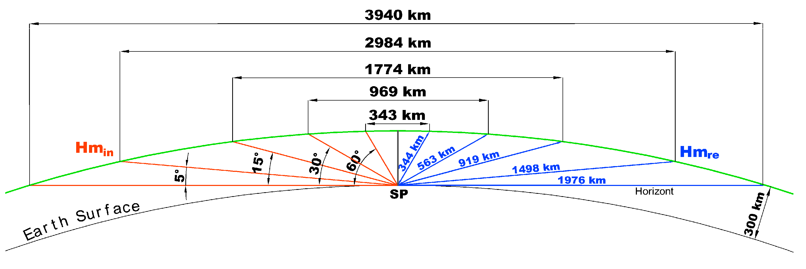
The LEO GNSS-R space-borne configuration, which enables the simultaneous collection of data from multiple reflections, presents several advantages for ionospheric studies. Firstly, thanks to the fast trajectory change of the LEO satellite, the GNSS-R signal rapidly scans along the ionospheric layers, providing a snapshot view of ionospheric structures [
8]. Secondly, the ability to obtain peak electron density points at different locations within a short time interval allows for the mapping of ionospheric structures at varying distances. Assuming the Earth’s radius is 6371 km, with a maximum electron density ionospheric shell at a 300 km height, the distance between the incident and reflected
points varies depending on the elevation angle as observed in
Figure 6.
4. Results
4.1. Slant Total Electron Content Analysis
The computed sTEC, obtained from the NEDM2020 and NeQuick 2 models, serves as the foundational parameter for the subsequent derivations of the relative ionospheric group delay and Doppler shift. The assessment of the sTEC is presented across different grazing elevation ranges: 5°–10° (very low), 10°–20° (low), and 20°–30°(mid-low), along with the distinct regions of north, tropics, and south. The outcomes of the NEDM2020 and NeQuick 2 sTEC computations during LSA are depicted in
Figure 7 and
Figure 8, respectively. While discrepancies of up to ~60 TECUs between the two models are noticeable in the tropics region at very low angles for the direct ray, both models consistently demonstrate similar behavior across all analyzed scenarios.
The highest sTEC is prominently observed at elevation angles ranging from 5° to 10° within the tropics region, and to a lesser extent in polar regions, but with lower magnitudes, specifically for the direct ray. This behavior occurs because, at such elevation angles, the direct ray traverses a longer path through the ionosphere than the incident and reflected rays. This effect diminishes as the elevation angle increases. At low elevations, the magnitudes of the sTEC are relatively similar for each ray, while at mid-low elevations, the contribution of the incident and reflected rays becomes more prominent in comparison to the direct ray.
Across all scenarios, local time, representing solar radiation, plays a pivotal role in sTEC retrievals.
Figure 7 and
Figure 8 illustrate how the sTEC values exhibit a progressive increase as the noon-time period approaches, with the highest peaks occurring between 12:00 and 13:00 h. Following sunset, the electron density and consequently the sTEC values gradually decrease accordingly.
Table 3 provides a comparative analysis of both models, presenting the mean and standard deviation values for each ray in the distinct regions. To facilitate interpretation in terms of local time, the events have been categorized into two distinct periods: daytime (DT), spanning from 06:00 to 18:00, and nighttime (NT), encompassing the interval from 18:00 to 06:00. Notably, the range of sTEC magnitude for the direct ray is broader for the NeQuick model computations in the tropics region. However, the NEDM2020 computations consistently yield a higher mean sTEC in most cases except for the direct ray at very low elevations in the tropics during daytime. Particularly higher differences in mean values between the two models are evident in the south region (~6 TECUs), while comparatively smaller differences are observed in the tropics region (~2 TECUs).
4.2. Relative Ionospheric Group Delay Analysis
The relative ionospheric group delay
denotes the additional delay caused by the ionosphere along the aggregated path of the incident and reflected signals, in comparison to the direct signal. The mitigation of ionospheric delay holds significant importance in reflectometry LEO single-frequency missions, particularly within altimetry applications. The analysis of the relative ionospheric delay follows a similar approach to the sTEC analysis, encompassing the established regions, elevation angle ranges, local time variations, and the change in solar flux index.
Figure 9 illustrates the potential ionospheric delays that arise from utilizing the sTEC derived from the NEDM2020 and NeQuick 2 models in conjunction with the GPS L1 frequency and F10.7 = 75.
Consistent with the sTEC analysis outcomes, it is observed that exhibits greater magnitudes within the tropics region, with the highest values occurring at very low elevation angles for both models. The occurrence of negative values in the relative ionospheric delay is attributed to the dominance of the direct signal contribution in the computation of .
While the outcomes from both models exhibit very similar behavior in terms of relative ionospheric delay, including their dependence on region, elevation angle, and local time, there are noticeable relative differences across the established groups. Taking as a reference the NEDM2020 model, the mean relative difference is computed as follows:
Table 4 presents the mean relative differences between low- and high-solar-activity conditions. During LSA, the most significant relative differences occur at very low elevation angles in both the north and south regions during nighttime, showing a notable 64% variation between the two models. This difference decreases as the elevation angle increases. Conversely, during daytime, the differences in the polar regions remain relatively consistent across all scenarios, while variations are more pronounced in the tropics region. During HSA, during nighttime in the north region, the differences can reach up to 98% at very low elevation angles, while in the south region, the differences remain relatively similar when comparing low and high solar activity. In the tropics, an increase in the F10.7 index leads to a higher relative difference between the models during nighttime. However, during daytime, this difference decreases compared to the low-solar-activity condition (F10.7 = 75).
The sTEC outcomes obtained from the NEDM2020 model, utilized as the reference model in this study, form the basis for the following analysis.
Figure 10 illustrates the ionospheric delay distribution during low solar activity, categorized by elevation angles, regions, and local time distinguishing between daytime and nighttime. At low and mid-low elevation angles, the contribution of each ray to the delay remains relatively similar in magnitude, resulting in positive values for the relative ionospheric delay. Overall, during daytime events, the
is on average 120% greater compared to nighttime events.
During HSA periods (F10.7 = 180), the relative ionospheric delay range can increase by up to 200% with respect to low-solar-activity periods, as seen in
Figure 11. In low- and mid-low-elevation scenarios, the distribution of
behaves similarly to LSA but with higher magnitude values. Notably, in the tropics region at very low elevations, the distribution is more widespread, with relative delays primarily consisting of negative values. This highlights the higher influence of the direct ray on
compared to low-solar-activity periods.
Group Delay Altimetry and Ionospheric Delay Uncertainty Analysis
As a single-frequency GNSS-R mission, PRETTY relies on ionospheric correction models to ensure precise sea surface height measurements, introducing a level of model uncertainty in the correction process.
Figure 12 presents the altimetric uncertainty at grazing elevation angles.
Figure 10 and
Figure 11 depict the distribution of the relative ionospheric delay, showing a noticeable diurnal cycle effect where daytime observations exhibit higher relative ionospheric delays compared to nighttime observations. This diurnal variation is also reflected in the sea surface height uncertainties. Furthermore, it is evident that ionospheric uncertainties have a significantly greater impact on sea height retrievals in the Tropics region, where the general level of ionization is higher. In this geographical area, we observe a higher altimetric uncertainty dispersion, particularly in the mid-low elevation angle regime (during daytime, 0.22 m mean and 4.08 m std), where the combined delay of the incident and reflected rays surpasses that of the direct ray. Consequently, this leads to higher relative delays and, by extension, a more pronounced impact on GNSS-R altimetric retrievals within this specific elevation range and region.
4.3. Doppler Shift Analysis
The analysis extends to the Doppler shift observed at the GPS L1 frequency across varying ranges of elevation angles, while considering effects during both day and night periods.
Figure 13 illustrates the distribution of the Doppler shift during low solar activity. The electron density variations in grazing angle reflectometry can induce a maximum Doppler shift of ±2 Hz in the GPS L1 signal during daytime. The attenuation in the Doppler shift demonstrates a strong correlation with diurnal cycles, resulting in a reduction during nighttime periods. This phenomenon can be attributed to the decrease in the rate of electron density changes, which in turn leads to a corresponding decrease in the magnitude of the Doppler shift.
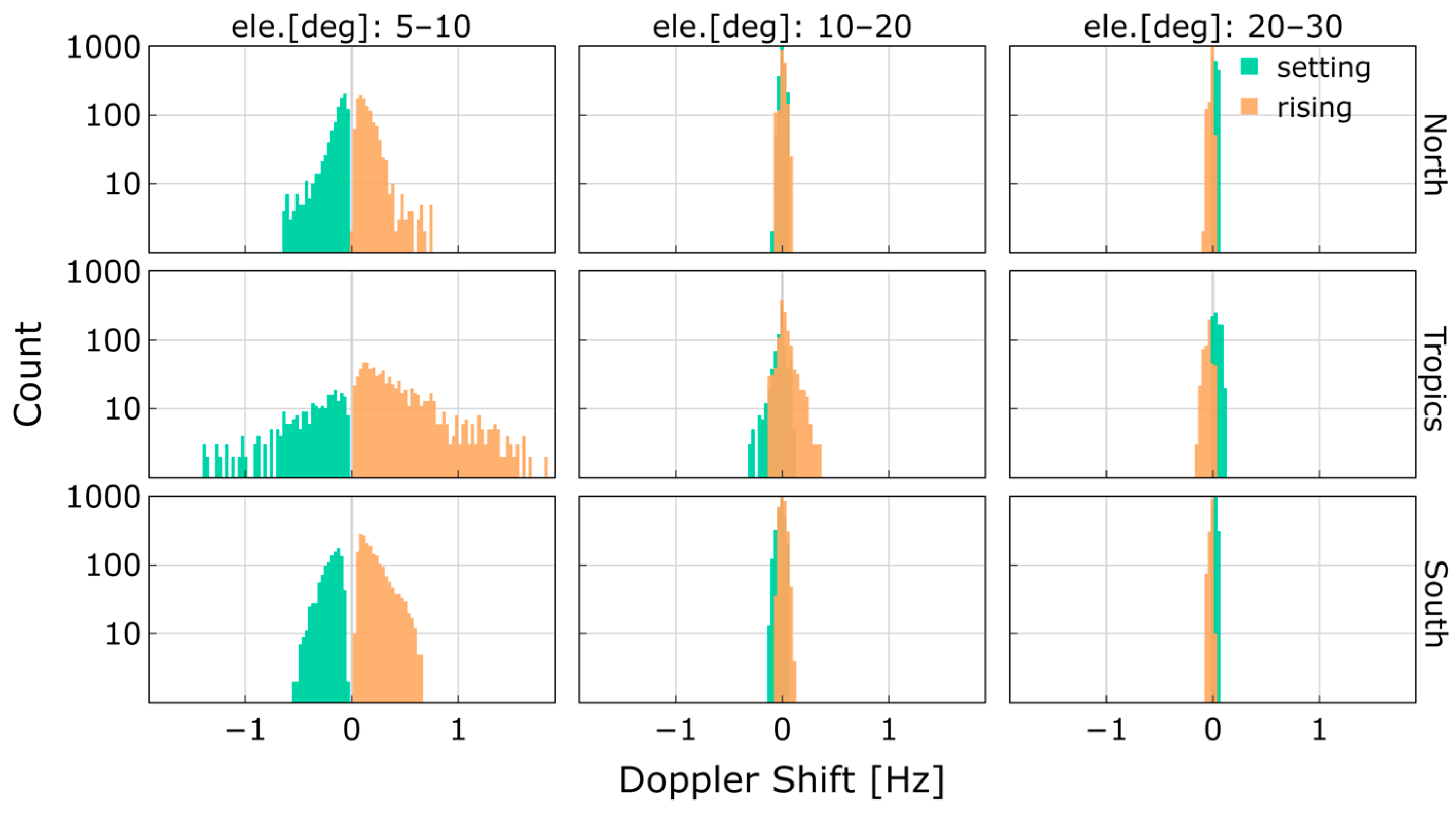
The Doppler shift histograms reveal a symmetrical distribution centered around approximately 0 Hz with a distinct separation in very-low-elevation cases. The distribution is also influenced by the transmitter motion relative to the specular point elevation angle. In
Figure 14, it becomes evident that at very low elevation angles, a rising transmitter (ascendant elevation) induces a positive Doppler shift, while a setting transmitter (descendant elevation) results in a negative Doppler shift. However, at higher elevation angles (20° to 30°), the relationship may vary or even reverse.
The distribution of the Doppler shift for F10.7 = 180 exhibits an increase in dispersion, approximately doubling in all scenarios. In the elevation range of 5°–10° within the tropics region, the range of is more extensive during daytime, reaching maximum values of up to ±4 Hz. The rising and setting event analyses present similar behavior, with negative magnitudes primarily observed during rising events and positive magnitudes during setting events.
4.4. Peak Electron Density Height Analysis
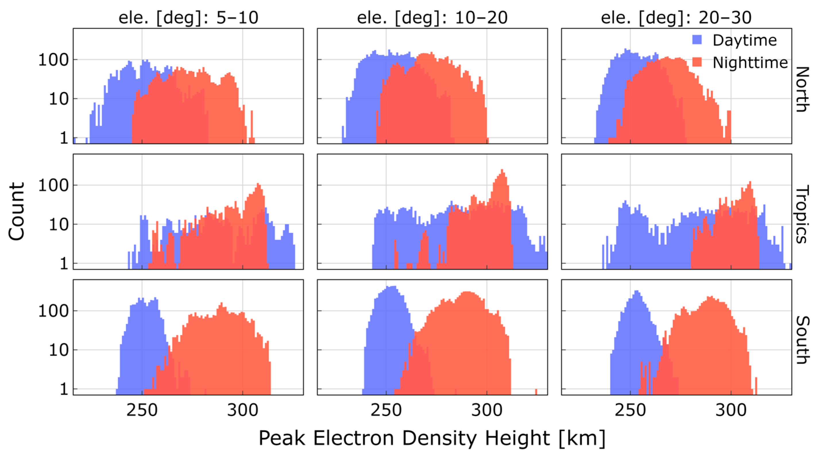
The NEDM2020 model is employed to determine the height at which the maximum electron density peak is observed along the paths of both the incident and reflected rays. This altitude is significant as it represents the point of maximum ionization within the ionosphere that the signals traverse.
From a geometrical standpoint within the grazing GNSS-R configuration, variations in elevation angles directly correspond to changes in the segment of the signal ray that travels along the ionosphere. Furthermore, throughout the diurnal cycle, electron densities within the E and F layers exhibit greater magnitudes during daylight hours compared to nighttime, with the F layer generally obtaining higher electron concentrations. These fluctuations are examined to comprehend the intricate ionospheric interactions that the signals undergo during their propagation. This phenomenon results in variations in the height of the maximum electron density peak, as depicted in
Figure 15 for both day and nighttime.
The overall average of the during the LSA period is 270 km. Nevertheless, noticeable variations are evident with respect to daytime and nighttime. In general, during nighttime, the is on average 10% higher than during daytime. The tropics region stands out as one of the most dynamically changing areas within the ionosphere. In this zone, the distribution of during daytime exhibits a spread ranging from 236 to 326 km, lacking a distinct peak value. However, during nighttime, reaches its maximum value at approximately 305 km. This highlights the substantial variations in electron density within this region, particularly during daytime. During HSA, the exhibits a consistent increase of 21% across all scenarios.
5. Discussion
The analysis provides valuable insights into how ionospheric parameters such as slant total electron content, relative ionospheric delay, Doppler shift, and peak electron density height vary in response to different conditions. These findings are crucial for optimizing the accuracy of space-borne GNSS-R applications, particularly in altimetry, aiding in the development of robust models, and enhancing the interpretation of data acquired through grazing GNSS-R configurations.
Under low-solar-activity conditions (F10.7 = 75), the resulting sTEC values from NEDM2020 and NeQuick 2 reveal that both models exhibit similar behavior across different scenarios. However, it is important to note that while an extensive evaluation of the models is not carried out in this study, differences in the sTEC computations and the relative total delay are observed. Significant differences of ~60 TECUs and up to 64% in relative ionospheric delay are observed in polar regions at very low elevation angles during daytime when comparing NEDM2020 and NeQuick 2. Under high-solar-activity conditions (F10.7 = 180), the relative differences can reach values up to 98%.
Grazing elevation angles, local time, regions, and solar activity emerge as the crucial factors determining ionospheric effects in GNSS-R. The observed elevation angle significantly influences the path traversed by GNSS signals through the ionosphere, while electron density variations rising from ionospheric diurnal cycles and geographical location contribute to fluctuations in the sTEC computation. The sTEC values exhibit a noticeable increase as the elevation angle decreases (very low to mid-low angles) in all regions during both daytime and nighttime.
Daytime events consistently result in higher sTEC values, larger relative ionospheric delay values, and higher Doppler shift magnitudes compared to nighttime events across all regions and elevation angles. The tropics region consistently displays the highest sTEC values across all elevation angle ranges, indicating the presence of higher electron densities. To provide a comprehensive synthesis of the study’s findings based on the electron density retrievals from the NEDM2020 model,
Table 5 and
Table 6 provide a summary of the results by presenting the median and standard deviation for each parameter outlined in the
Section 4 for F10.7 = 75 and F10.7 = 180, respectively. The parameters provided by the summary tables are the relative ionospheric delay
in meters, absolute value of Doppler shift
in Hertz, and peak electron density height
) in kilometers.
In general, as the F10.7 index increases, notable observations emerge: (1) There is a compensation effect, attributed to the direct signal contribution, leading to a decrease in the median level of relative ionospheric delay as elevation decreases, particularly at very low elevations. (2) The absolute Doppler shift exhibits a substantial increase in median values, scaling up to one order of magnitude, as elevation angles decrease to their lowest. (3) Notably, in tropical regions characterized by higher density peak heights, there is a more pronounced compensation by direct signal contribution in at the lowest elevations, resulting in negative median delay values.
For a LEO GNSS-R mission employing the GPS L1 frequency, findings show that relative ionospheric delays can reach ~19 m during periods of LSA and ~70 m during HSA, equivalent to about 120 and 430 TECUs. The forthcoming ESA PRETTY mission will pioneer grazing altimetry at the L5 frequency, which, with its longer wavelength (~0.2548 m), is more sensitive to ionospheric group delays. Using 120 and 430 TECUs as benchmarks, relative ionospheric corrections of approximately 35 and 125 m can be expected for group delay altimetry during low and high solar activity.
6. Conclusions
In this paper, we have analyzed ionospheric effects in GNSS-R at grazing angles. This study encompasses the characterization of slant total electron content, relative ionospheric delay, the influence of ionospheric correction model uncertainties on GNSS-R group delay altimetry retrievals, the Doppler effect, and peak electron density height changes. Various factors have been considered such as satellite geometry, latitude-dependent regions, temporal variations, and solar activity.
When analyzing the results during LSA (low solar activity) and HSA (high solar activity), it becomes evident that as the elevation decreases into the grazing regime below 20°, the median relative ionospheric delay decreases due to the compensation from the direct signal contribution. However, it is important to note that the standard deviation of the delay, especially in terms of the Doppler shift, undergoes a substantial increase. This behavior poses a significant challenge for the model-based correction of ionospheric delay in GNSS reflectometry altimetry at grazing elevation angles.
While model uncertainties do affect group delay sea height estimates it is important to highlight that these effects are not uniform across all GNSS-R observations. Coherent phase observations, for instance, offer a remarkable level of precision, down to the centimeter scale. Along reflection tracks characterized by consistent ionospheric bias, relative altimetry at a centimeter precision level can be achieved. This means that even in the presence of ionospheric delay bias, LEO space-borne GNSS-R systems, as reported in [
26], can still provide precise results in the altimetric inversion.
Total electron content, a crucial ionospheric parameter, exhibits complex variations spanning diurnal, monthly, seasonal, and 11-year solar cycles. Extended temporal coverage is essential for deciphering these patterns, especially in dynamic regions allowing analysis of seasonal trends. This study highlights the importance of spatially extended data, particularly in tropical areas with substantial ionospheric variability. Such data is key to comprehending ionospheric parameter evolution across different time scales and regions, influenced by factors like solar activity and geomagnetic storms.
GNSS-R (global navigation satellite system reflectometry) stands as a valuable and complementary remote sensing tool in ionospheric studies, effectively addressing areas not covered by alternative methods. This capacity offers significant contributions to the modeling, prediction, and comprehension of ionospheric effects.
Author Contributions
Conceptualization: M.M., M.S. and G.S.; methodology: M.M., M.S. and G.S.; software: M.M. and M.S.; data resources: M.M. and M.S.; writing—original draft preparation: M.M.; writing—review and editing: M.S., G.S., M.H. and J.W.; visualization, M.M.; supervision, M.S., J.W. and M.H. All authors have read and agreed to the published version of the manuscript.
Funding
This research was funded by the German Aerospace Center, Institute for Solar-Terrestrial Physics (DLR-SO).
Data Availability Statement
Data are available under the authorization of Spire Global Inc.
Acknowledgments
The authors would like to thank Spire Global for providing real orbit from Lemur-2 constellation LEO satellites.
Conflicts of Interest
The authors declare no conflict of interest. The funders had no role in the design of the study; in the collection, analyses, or interpretation of data; in the writing of the manuscript, or in the decision to publish the results.
References
- Hagfors, T. 2.1. The Ionosphere. In Methods in Experimental Physics; Meeks, M.L., Ed.; Astrophysics; Academic Press: Cambridge, MA, USA, 1976; Volume 12, pp. 119–135. [Google Scholar]
- Dubey, S.; Wahi, R.; Gwal, A.K. Ionospheric Effects on GPS Positioning. Adv. Space Res. 2006, 38, 2478–2484. [Google Scholar] [CrossRef]
- Wickert, J.; Michalak, G.; Schmidt, T.; Beyerle, G.; Cheng, C.Z.; Healy, S.B.; Heise, S.; Huang, C.Y.; Jakowski, N.; Kohler, W.; et al. GPS Radio Occultation: Results from CHAMP. GRACE and FORMOSAT-3/COSMIC. Terr. Atmos. Ocean. Sci. 2009, 20, 35–50. [Google Scholar] [CrossRef]
- Xing, J.; Datta-Barua, S.; Garrison, J.; Ridley, A.; Pervan, B. Relative Ionospheric Ranging Delay in LEO GNSS Oceanic Reflections. IEEE Geosci. Remote Sens. Lett. 2015, 12, 1416–1420. [Google Scholar] [CrossRef]
- Ruf, C.; Gleason, S.; Jelenak, Z.; Katzberg, S.; Ridley, A.; Rose, R.; Scherrer, J.; Zavorotny, V. The NASA EV-2 Cyclone Global Navigation Satellite System (CYGNSS) Mission. In Proceedings of the 2013 IEEE Aerospace Conference, Big Sky, MT, USA, 2–9 March 2013; pp. 1–7. [Google Scholar]
- Camps, A.; Park, H.; Foti, G.; Gommenginger, C. Ionospheric Effects in GNSS-Reflectometry From Space. IEEE J. Sel. Top. Appl. Earth Obs. Remote Sens. 2016, 9, 5851–5861. [Google Scholar] [CrossRef]
- Unwin, M.; Jales, P.; Tye, J.; Gommenginger, C.; Foti, G.; Rosello, J. Spaceborne GNSS-Reflectometry on TechDemoSat-1: Early Mission Operations and Exploitation. IEEE J. Sel. Top. Appl. Earth Obs. Remote Sens. 2016, 9, 4525–4539. [Google Scholar] [CrossRef]
- Wang, Y.; Morton, Y.J. Ionospheric Total Electron Content and Disturbance Observations From Space-Borne Coherent GNSS-R Measurements. IEEE Trans. Geosci. Remote Sens. 2022, 60, 1–13. [Google Scholar] [CrossRef]
- Liu, L.; Morton, Y.J.; Wang, Y.; Wu, K.-B. Arctic TEC Mapping Using Integrated LEO-Based GNSS-R and Ground-Based GNSS Observations: A Simulation Study. IEEE Trans. Geosci. Remote Sens. 2022, 60, 1–10. [Google Scholar] [CrossRef]
- Roesler, C.; Wang, Y.; Morton, Y.J.; Nerem, R.S. Coherent GPS Reflections Over Ocean Surface. In Proceedings of the IGARSS 2020–2020 IEEE International Geoscience and Remote Sensing Symposium, Waikoloa, HI, USA, 26 September–2 October 2020; pp. 6218–6221. [Google Scholar]
- Moreno, M.; Semmling, M.; Stienne, G.; Dalil, W.; Hoque, M.; Wickert, J.; Reboul, S. Airborne Coherent GNSS Reflectometry and Zenith Total Delay Estimation over Coastal Waters. Remote Sens. 2022, 14, 4628. [Google Scholar] [CrossRef]
- Issa, H.; Stienne, G.; Reboul, S.; Raad, M.; Faour, G. Airborne GNSS Reflectometry for Water Body Detection. Remote Sens. 2021, 14, 163. [Google Scholar] [CrossRef]
- Subirana, J.S.; Zornoza, J.M.J.; Hernández-Pajares, M. GNSS Data Processing; Contactivity bv; ESA Communications: Leiden, The Netherlands, 2013; Volume I, Fundamentals and Algorithms; ISBN 978-92-9221-886-7. [Google Scholar]
- Hoque, M.M.; Jakowski, N.; Osechas, O.; Berdermann, J. Fast and Improved Ionospheric Correction for Galileo Mass Market Receivers. In Proceedings of the 32nd International Technical Meeting of the Satellite Division of the Institute of Navigation (ION GNSS+ 2019), Miami, FL, USA, 11 October 2019; pp. 3377–3389. [Google Scholar]
- Nava, B.; Coïsson, P.; Radicella, S.M. A New Version of the NeQuick Ionosphere Electron Density Model. J. Atmos. Sol. Terr. Phys. 2008, 70, 1856–1862. [Google Scholar] [CrossRef]
- Ionospheric Correction Algorithms|European GNSS Service Centre. Available online: https://www.gsc-europa.eu/support-to-developers/ionospheric-correction-algorithms (accessed on 27 July 2023).
- Dielacher, A.; Fragner, H.; Koudelka, O. PRETTY—Passive GNSS-Reflectometry for CubeSats. Elektrotech. Inftech. 2022, 139, 25–32. [Google Scholar] [CrossRef]
- Hoque, M.M.; Jakowski, N.; Prol, F.S. A New Climatological Electron Density Model for Supporting Space Weather Services. J. Space Weather Space Clim. 2022, 12, 1. [Google Scholar] [CrossRef]
- Nguyen, V.; Jales, P.; Garbacz, H. Spire Earth Observations for NASA’s CSDA Program—Lunch & Learn. 2022. Available online: https://www.earthdata.nasa.gov/s3fs-public/2022-10/2022%2010%2006%20Spire%20Earth%20Observations%20for%20NASA%27s%20CSDA%20Program%20-%20Lunch%20%26%20Learn_0.pdf (accessed on 20 July 2023).
- Semmling, A.M.; Leister, V.; Saynisch, J.; Zus, F.; Heise, S.; Wickert, J. A Phase-Altimetric Simulator: Studying the Sensitivity of Earth-Reflected GNSS Signals to Ocean Topography. IEEE Trans. Geosci. Remote Sens. 2016, 54, 6791–6802. [Google Scholar] [CrossRef]
- Hoque, M.M.; Jakowski, N.; Cahuasquí, J.A. Fast Ionospheric Correction Algorithm for Galileo Single Frequency Users. In Proceedings of the 2020 European Navigation Conference (ENC), Dresden, Germany, 23–24 November 2020; pp. 1–10. [Google Scholar]
- Cardellach, E.; Ao, C.O.; de la Torre Juárez, M.; Hajj, G.A. Carrier Phase Delay Altimetry with GPS-Reflection/Occultation Interferometry from Low Earth Orbiters. Geophys. Res. Lett. 2004, 31. [Google Scholar] [CrossRef]
- Mashburn, J.; Axelrad, P.; Lowe, S.T.; Larson, K.M. Global Ocean Altimetry With GNSS Reflections From TechDemoSat-1. IEEE Trans. Geosci. Remote Sens. 2018, 56, 4088–4097. [Google Scholar] [CrossRef]
- Davies, K.; Watts, J.M.; Zacharisen, D.H. A Study of F 2-Layer Effects as Observed with a Doppler Technique. J. Geophys. Res. 1962, 67, 601–609. [Google Scholar] [CrossRef]
- Jacobs, J.A.; Watanabe, T. Doppler Frequency Changes in Radio Waves Propagating Through a Moving Ionosphere. Radio Sci. 1966, 1, 257–264. [Google Scholar] [CrossRef]
- Cardellach, E.; Li, W.; Rius, A.; Semmling, M.; Wickert, J.; Zus, F.; Ruf, C.S.; Buontempo, C. First Precise Spaceborne Sea Surface Altimetry With GNSS Reflected Signals. IEEE J. Sel. Top. Appl. Earth Obs. Remote Sens. 2020, 13, 102–112. [Google Scholar] [CrossRef]
- Teunissen, P.J.G.; Kleusberg, A. GPS Observation Equations and Positioning Concepts. In GPS for Geodesy; Kleusberg, A., Teunissen, P.J.G., Eds.; Lecture Notes in Earth Sciences; Springer: Berlin/Heidelberg, Germany, 1996; pp. 175–217. ISBN 978-3-540-49447-8. [Google Scholar]
Figure 1.
(a) LEO GNSS-R representation at 30° elevation angle at specular point. (b) LEO GNSS-R representation at 5° elevation angle. denotes the slant total electron content. Subscripts dr, in, and re correspond to the direct ray (transmitter to receiver ), incident ray (transmitter to specular point ), and reflected ray (specular point to receiver), respectively. represents the peak electron density height for the incident and reflected ray paths.
Figure 2.
Specular point tracks provided by the Spire Lemur-2 CubeSats on 1 March 2021, color-coded according to coordinated universal time (UTC) in hours.
Figure 2.
Specular point tracks provided by the Spire Lemur-2 CubeSats on 1 March 2021, color-coded according to coordinated universal time (UTC) in hours.
Figure 3.
Representation of the specular point change along track (blue stars) for the SVN 79 and PRN 30 every 10 s (~45 km) and the ray points every 10 km along the direct, incident, and reflected ray paths (red dots).
Figure 3.
Representation of the specular point change along track (blue stars) for the SVN 79 and PRN 30 every 10 s (~45 km) and the ray points every 10 km along the direct, incident, and reflected ray paths (red dots).
Figure 4.
(a) Total number of reflection events on 1 March 2021 by region. (b) The number of reflection events across grazing angles, ranging from 5° to 30°.
Figure 4.
(a) Total number of reflection events on 1 March 2021 by region. (b) The number of reflection events across grazing angles, ranging from 5° to 30°.
Figure 5.
Electron density variations along the change and model profile comparison for the incident, reflected, and direct rays at very low and mid-low elevation angles (F10.7 = 75).
Figure 5.
Electron density variations along the change and model profile comparison for the incident, reflected, and direct rays at very low and mid-low elevation angles (F10.7 = 75).
Figure 6.
Distances between peak electron density height points depending on the elevation angle change at 300 km height.
Figure 6.
Distances between peak electron density height points depending on the elevation angle change at 300 km height.
Figure 7.
sTEC obtained from NEDM2022 model. Color-coded according to the direct (dr), incident (in), and reflected (re) rays.
Figure 7.
sTEC obtained from NEDM2022 model. Color-coded according to the direct (dr), incident (in), and reflected (re) rays.
Figure 8.
sTEC obtained from NeQuick 2 model. Color-coded according to the direct (dr), incident (in), and reflected (re) rays.
Figure 8.
sTEC obtained from NeQuick 2 model. Color-coded according to the direct (dr), incident (in), and reflected (re) rays.
Figure 9.
Relative ionospheric delay in the distinct regions and grazing angle elevation ranges along with local time variations.
Figure 9.
Relative ionospheric delay in the distinct regions and grazing angle elevation ranges along with local time variations.
Figure 10.
Distribution of relative ionospheric delay depending on elevation, daytime (DT), and nighttime (NT) using NEDM2020 sTEC retrievals with F10.7 = 75.
Figure 10.
Distribution of relative ionospheric delay depending on elevation, daytime (DT), and nighttime (NT) using NEDM2020 sTEC retrievals with F10.7 = 75.
Figure 11.
Distribution of relative ionospheric delay depending on elevation, daytime (DT), and nighttime (NT) using NEDM2020 sTEC retrievals with F10.7 = 180.
Figure 11.
Distribution of relative ionospheric delay depending on elevation, daytime (DT), and nighttime (NT) using NEDM2020 sTEC retrievals with F10.7 = 180.
Figure 12.
Altimetric uncertainty due to uncertainty in ionospheric delay model depending on elevation, daytime (DT), and nighttime (NT) using NEDM2020 during LSA.
Figure 12.
Altimetric uncertainty due to uncertainty in ionospheric delay model depending on elevation, daytime (DT), and nighttime (NT) using NEDM2020 during LSA.
Figure 13.
Distribution of Doppler shift depending on elevation, daytime (DT), and nighttime (NT) using NEDM2020 sTEC retrievals with F10.7 = 75.
Figure 13.
Distribution of Doppler shift depending on elevation, daytime (DT), and nighttime (NT) using NEDM2020 sTEC retrievals with F10.7 = 75.
Figure 14.
Distribution of Doppler shift depending on elevation and rising or setting event using NEDM2020 sTEC retrievals with F10.7 = 75.
Figure 14.
Distribution of Doppler shift depending on elevation and rising or setting event using NEDM2020 sTEC retrievals with F10.7 = 75.
Figure 15.
Peak electron density height variations depending on elevation ranges, regions, and day and nighttime using NEDM2020 sTEC retrievals with F10.7 = 75.
Figure 15.
Peak electron density height variations depending on elevation ranges, regions, and day and nighttime using NEDM2020 sTEC retrievals with F10.7 = 75.
Table 1.
Total number of events per region and durations.
Table 1.
Total number of events per region and durations.
| Region | Number of Events | Total Minutes |
|---|
| North | 474 | 1704 |
| Tropics | 168 | 760 |
| South | 546 | 2335 |
| Total | 1188 | 4798 |
Table 2.
Space Vehicle Numbers of Lemur-2 CubeSats and GPS Satellite PRNs on 01/03/2021.
Table 2.
Space Vehicle Numbers of Lemur-2 CubeSats and GPS Satellite PRNs on 01/03/2021.
| | Spire SVN | GPS PRN |
|---|
| | 79, 84, 99, 100, 101, 102, 103, 104, 106, 113, 115, 116, 117, 119, 120, 121, 122, 124, 125, 128, 129 | 1, 3, 5, 6, 7, 8, 9, 10, 12, 15, 17, 24, 25, 26, 27, 29, 30, 31, 32 |
| Total | 21 | 19 |
Table 3.
sTEC mean and standard deviation value comparison between NEDM2020 and NeQuick 2 models for F10.7 = 75.
Table 3.
sTEC mean and standard deviation value comparison between NEDM2020 and NeQuick 2 models for F10.7 = 75.
| | | sTEC NEDM (TECU) | sTEC NeQuick 2 (TECU) |
|---|
| | | Ele.: 5°–10° | Ele.: 10°–20° | Ele.: 20°–30° | Ele.: 5°–10° | Ele.: 10°–20° | Ele.: 20°–30° |
|---|
| | | dr | in | re | dr | in | re | dr | in | re | dr | in | re | dr | in | re | dr | in | re |
|---|
| North | | | | | | | | | | | | | | | | | | | |
| DT | mean | 28 | 26 | 23 | 8 | 20 | 18 | 3 | 14 | 13 | 21 | 19 | 17 | 6 | 15 | 13 | 3 | 11 | 9 |
| std | 13 | 8 | 11 | 3 | 8 | 7 | 1 | 6 | 5 | 12 | 8 | 9 | 3 | 7 | 6 | 1 | 5 | 4 |
| NT | mean | 21 | 16 | 13 | 7 | 13 | 11 | 3 | 9 | 8 | 14 | 8 | 7 | 4 | 7 | 5 | 2 | 6 | 4 |
| std | 10 | 4 | 3 | 3 | 4 | 2 | 1 | 3 | 1 | 7 | 3 | 2 | 2 | 2 | 2 | 1 | 2 | 1 |
| Tropics | | | | | | | | | | | | | | | | | | | |
| DT | mean | 121 | 72 | 63 | 33 | 62 | 52 | 16 | 48 | 39 | 126 | 63 | 60 | 31 | 57 | 49 | 14 | 43 | 37 |
| std | 55 | 16 | 11 | 17 | 16 | 12 | 6 | 14 | 10 | 67 | 20 | 19 | 16 | 22 | 17 | 6 | 19 | 14 |
| NT | mean | 43 | 29 | 20 | 17 | 27 | 18 | 10 | 22 | 15 | 40 | 26 | 16 | 14 | 27 | 17 | 8 | 21 | 16 |
| std | 25 | 9 | 7 | 7 | 7 | 6 | 3 | 6 | 4 | 35 | 16 | 12 | 10 | 16 | 11 | 6 | 12 | 10 |
| South | | | | | | | | | | | | | | | | | | | |
| DT | mean | 43 | 34 | 32 | 13 | 28 | 25 | 6 | 22 | 18 | 31 | 26 | 25 | 10 | 22 | 20 | 5 | 17 | 14 |
| std | 16 | 8 | 6 | 5 | 7 | 5 | 1 | 5 | 4 | 14 | 7 | 5 | 3 | 6 | 4 | 1 | 4 | 3 |
| NT | mean | 29 | 20 | 16 | 10 | 17 | 14 | 5 | 13 | 11 | 15 | 10 | 7 | 5 | 8 | 6 | 2 | 7 | 5 |
| std | 10 | 4 | 3 | 4 | 3 | 2 | 1 | 2 | 2 | 8 | 4 | 3 | 2 | 3 | 2 | 1 | 2 | 2 |
Table 4.
Mean relative difference in the relative ionospheric delay between NEDM2020 and NeQuick 2 during high and low solar activity.
Table 4.
Mean relative difference in the relative ionospheric delay between NEDM2020 and NeQuick 2 during high and low solar activity.
| | LSA (F10.7 = 75) | HSA (F10.7 = 180) |
|---|
| | Ele.: 5°–10° | Ele.: 10°–20° | Ele.: 20°–30° | Ele.: 5°–10° | Ele.: 10°–20° | Ele.: 20°–30° |
|---|
| North | | | | | | |
| DT | 30% | 28% | 26% | 59% | 17% | 15% |
| NT | 64% | 49% | 46% | 98% | 38% | 28% |
| Tropics | | | | | | |
| DT | 48% | 17% | 17% | 27% | 16% | 14% |
| NT | 58% | 35% | 38% | 88% | 76% | 48% |
| South | | | | | | |
| DT | 19% | 21% | 23% | 41% | 21% | 24% |
| NT | 64% | 53% | 51% | 66% | 56% | 51% |
Table 5.
Overview of ionospheric parameters from the NEDM2020 sTEC computations during low solar activity (F10.7 = 75).
Table 5.
Overview of ionospheric parameters from the NEDM2020 sTEC computations during low solar activity (F10.7 = 75).
| | | Very Low: 5°–10° | Low: 10°–20° | Mid-Low: 20°–30° |
|---|
| | | | | | | | | | | |
|---|
| | | (m) | (Hz) | (km) | (m) | (Hz) | (km) | (m) | (Hz) | (km) |
|---|
| North | | | | | | | | | | |
| DT | median | 3.10 | 0.133 | 251.7 | 4.35 | 0.022 | 252.3 | 3.33 | 0.026 | 252.2 |
| std | 1.96 | 0.142 | 11.7 | 1.81 | 0.019 | 10.5 | 1.44 | 0.021 | 8.5 |
| NT | median | 1.38 | 0.097 | 274.0 | 2.61 | 0.009 | 271.9 | 2.27 | 0.011 | 268.3 |
| std | 1.19 | 0.067 | 12.9 | 0.60 | 0.014 | 11.6 | 0.47 | 0.006 | 9.7 |
| Tropics | | | | | | | | | | |
| DT | median | 3.96 | 0.729 | 287.9 | 13.50 | 0.048 | 287.4 | 12.12 | 0.067 | 285.3 |
| std | 7.57 | 0.415 | 21.4 | 2.61 | 0.070 | 22.4 | 2.87 | 0.028 | 23.8 |
| NT | median | 1.63 | 0.219 | 302.6 | 4.95 | 0.016 | 305.4 | 4.74 | 0.014 | 305.4 |
| std | 2.82 | 0.195 | 13.1 | 1.18 | 0.033 | 9.1 | 1.05 | 0.013 | 7.3 |
| South | | | | | | | | | | |
| DT | median | 3.98 | 0.220 | 252.2 | 6.49 | 0.030 | 252.2 | 5.63 | 0.014 | 253.1 |
| std | 2.26 | 0.138 | 5.2 | 1.15 | 0.021 | 5.2 | 1.02 | 0.022 | 4.9 |
| NT | median | 1.41 | 0.145 | 289.0 | 3.36 | 0.012 | 288.8 | 3.17 | 0.015 | 289.1 |
| std | 1.27 | 0.073 | 11.2 | 0.48 | 0.021 | 9.8 | 0.40 | 0.007 | 9.2 |
Table 6.
Overview of ionospheric parameters from the NEDM2020 sTEC computations during high solar activity (F10.7 = 180).
Table 6.
Overview of ionospheric parameters from the NEDM2020 sTEC computations during high solar activity (F10.7 = 180).
| | | Very Low: 5°–10° | Low: 10°–20° | Mid-Low: 20°–30° |
|---|
| | | | | | | | | | | |
|---|
| | | (m) | (Hz) | (km) | (m) | (Hz) | (km) | (m) | (Hz) | (km) |
|---|
| North | | | | | | | | | | |
| DT | median | 2.77 | 0.516 | 306.8 | 9.18 | 0.075 | 307.6 | 8.09 | 0.049 | 307.5 |
| std | 6.00 | 0.496 | 13.9 | 4.24 | 0.085 | 12.7 | 3.79 | 0.043 | 10.4 |
| NT | median | 0.03 | 0.330 | 333.8 | 5.11 | 0.051 | 331.7 | 5.31 | 0.015 | 327.2 |
| std | 3.90 | 0.148 | 15.9 | 1.64 | 0.066 | 14.4 | 1.16 | 0.011 | 12.0 |
| Tropics | | | | | | | | | | |
| DT | median | −21.45 | 2.329 | 349.5 | 25.56 | 0.246 | 348.4 | 28.45 | 0.139 | 345.2 |
| std | 24.43 | 0.698 | 26.7 | 9.30 | 0.377 | 27.3 | 5.96 | 0.068 | 28.9 |
| NT | median | −5.21 | 0.817 | 368.1 | 8.82 | 0.144 | 371.9 | 11.55 | 0.022 | 371.9 |
| std | 9.88 | 0.352 | 15.7 | 3.74 | 0.173 | 10.9 | 2.40 | 0.024 | 8.8 |
| South | | | | | | | | | | |
| DT | median | 1.46 | 0.812 | 307.2 | 13.57 | 0.084 | 306.9 | 13.97 | 0.037 | 307.9 |
| std | 7.58 | 0.333 | 6.5 | 3.39 | 0.109 | 6.4 | 2.62 | 0.043 | 6.0 |
| NT | median | −1.98 | 0.472 | 351.7 | 6.26 | 0.081 | 351.2 | 7.17 | 0.015 | 351.8 |
| std | 3.99 | 0.146 | 14.1 | 1.84 | 0.092 | 12.3 | 0.92 | 0.015 | 11.4 |
| Disclaimer/Publisher’s Note: The statements, opinions and data contained in all publications are solely those of the individual author(s) and contributor(s) and not of MDPI and/or the editor(s). MDPI and/or the editor(s) disclaim responsibility for any injury to people or property resulting from any ideas, methods, instructions or products referred to in the content. |
© 2023 by the authors. Licensee MDPI, Basel, Switzerland. This article is an open access article distributed under the terms and conditions of the Creative Commons Attribution (CC BY) license (https://creativecommons.org/licenses/by/4.0/).

 ,
, 


