Article

Classification of High-Altitude Flying Objects Based on Radiation Characteristics with Attention-Convolutional Neural Network and Gated Recurrent Unit Network

1
State Key Laboratory of Laser Interaction with Matter, Changchun Institute of Optics, Fine Mechanics and Physics, Chinese Academy of Sciences, Changchun 130033, China
2
University of Chinese Academy of Sciences, Beijing 100049, China
*
Author to whom correspondence should be addressed.
Remote Sens. 2023, 15(20), 4985; https://doi.org/10.3390/rs15204985
Submission received: 27 September 2023 / Revised: 10 October 2023 / Accepted: 11 October 2023 / Published: 16 October 2023

Abstract

:
In the task of classifying high-altitude flying objects, due to the limitations of the target flight altitude, there are issues such as insufficient contour information, low contrast, and fewer pixels in the target objects obtained through infrared detection technology, making it challenging to accurately classify them. In order to improve the classification performance and achieve the effective classification of the targets, this study proposes a high-altitude flying object classification algorithm based on radiation characteristic data. The target images are obtained through an infrared camera, and the radiation characteristics of the targets are measured using radiation characteristic measurement techniques. The classification is performed using an attention-based convolutional neural network (CNN) and gated recurrent unit (GRU) (referred to as ACGRU). In ACGRU, CNN-GRU and GRU-CNN networks are used to extract vectorized radiation characteristic data. The raw data are processed using Highway Network, and SoftMax is used for high-altitude flying object classification. The classification accuracy of ACGRU reaches 94.8%, and the F1 score reaches 93.9%. To verify the generalization performance of the model, comparative experiments and significance analysis were conducted with other algorithms on radiation characteristic datasets and 17 multidimensional time series datasets from UEA. The results show that the proposed ACGRU algorithm performs excellently in the task of high-altitude flying object classification based on radiation characteristics.

1. Introduction

The classification of high-altitude flying objects has important applications in air traffic safety management [1], air defense and missile defense, etc. The main types of high-altitude flying objects include birds, aircraft, and missiles. Accurately identifying birds can provide accurate information for bird control, ensuring flight safety for aircraft. Rapidly identifying enemy aircraft and missiles can provide strategic information in a timely manner, ensuring national security. Being able to quickly and accurately distinguish the type of flying objects is a pressing problem that needs to be solved.
Infrared detection technology is an important technology in target detection and other defense fields. It has the advantages of all-weather operation and high reliability, making it suitable for passive detection. Due to the high sensitivity and penetration ability of infrared cameras to heat sources, these can detect the radiation of target heat at relatively long distances. Compared to regular cameras, infrared cameras can provide more accurate imaging information, especially in high-altitude monitoring. Therefore, many scholars use infrared imaging to detect high-altitude targets. For example, Deng et al. [2] improved the top-hat transform technique to address the difficulty of detecting small targets using this method and applied it to small target detection in infrared images. The results show that the proposed method effectively detects small targets in infrared images. In addition, Zhang et al. [3] proposed a self-regularized weighted sparse model that uses the overlapping edges of the background structure information in infrared images to constrain the sparse items, thereby improving the accuracy of target detection. Ju et al. [4] proposed the ISTDet model, which detects infrared images using an infrared filtering module and an infrared small-target detection module, achieving excellent results. Li et al. [5] proposed a dense nested attention network for single-frame infrared images, which can separate small targets from cluttered backgrounds. They conducted experiments on their self-built dataset and compared it with publicly available datasets, achieving superior performance. Most of the scholars mentioned above detect infrared targets based on their single morphological features. Although these scholars can effectively identify the presence of targets in the spatial domain using clever methods, it is difficult to distinguish them based on shape and contour features due to the low contrast of small targets appearing as fewer pixels in infrared images.
The infrared radiation characteristics of high-altitude flying objects are crucial for target detection, recognition, and tracking [6]. The infrared radiation characteristics of these flying objects are determined by their temperature and surface properties. Higher temperatures result in more and stronger infrared radiation. Different surface materials have varying degrees of the absorption and reflection of infrared radiation, which also affects the infrared radiation characteristics of the flying objects, thereby forming the infrared spectrum of the object and providing characteristic information about the object. With the growing demand for infrared technology in the aviation field, more and more experts are conducting research on the infrared radiation characteristics of flying objects. Wang et al. [7] proposed a method based on the judgment of target-effective imaging pixels for measuring infrared radiation, distinguishing between small targets and surface targets. Kou et al. [8] established a dynamic feature model to study the correlation between infrared radiation characteristic signals and target maneuvering modes. Chen et al. [9] studied the variation in the infrared radiation brightness of the sky background under different weather conditions, providing a reference value for infrared target detection and recognition. These experts have made important contributions to the measurement of infrared radiation from ground to air. Considering that targets with low contrast in infrared images are difficult to distinguish based on morphological features, infrared radiation measurement techniques can be used to obtain target radiation information through radiation inversion, thereby facilitating target detection and recognition.
The methods for classifying high-altitude flying objects can be divided into traditional machine learning methods and deep learning methods. After processing the data source, traditional machine learning methods such as Bayesian decision [10], K-nearest neighbors [11], and support vector machine [12] are used for classification, or the original data source is subjected to feature extraction using deep learning methods based on CNN [13] or RNN [14]. Traditional machine learning methods have flexibility in feature engineering and can manually design suitable features according to the problem, making them applicable to small samples and high-dimensional data. However, traditional machine learning methods are limited by the constraints of manual feature extraction and may not be able to discover complex data relationships and patterns. In contrast, deep learning methods based on deep learning can automatically learn and extract higher-level and more abstract features from raw data. In deep learning, CNN-based methods are suitable for processing static data and can identify spatial and location-related features, but they cannot capture temporal information. RNN-based methods can handle time series data and model temporal dependencies, but these may face problems of gradient vanishing and exploding when dealing with long-term dependencies or long sequences [15].
When facing the task of time-series data classification, combining convolutional neural networks (CNNs) and recurrent neural networks (RNNs) can fully utilize the strengths of both neural networks. This approach enables the handling of variable-sized inputs, capturing spatial and temporal dependencies, enhancing feature extraction capabilities, and mitigating the problem of vanishing gradients. By doing so, the performance of time-series data classification is improved. For example, Zhu et al. [16] applied the SeqGAN-based text generation oversampling technique to expand the Self-Admitted Technical Debt (SATD) dataset for SATD recognition tasks. They serialized the SATD data sample vectors and padded them to a uniform length. The proposed convolutional neural networks-gated recurrent unit model was employed for classification, successfully identifying multiple categories of SATD and assisting with accurate debt localization. Cai et al. [17] proposed a parallel fusion method based on CNN and GRU for classifying power quality disturbances (PQDs) in complex power grid environments. CNN was used to extract the short-term features of PQDs, while GRU was used to extract long-term features. The features extracted through CNN and GRU were simultaneously fused and transmitted to SoftMax for classification. Simulation results showed that this method achieved a high classification accuracy. In the context of classifying elderly heartbeat sounds, Yadav et al. [18] augmented and expanded the heart sound database and proposed an algorithm based on CNN and bidirectional GRU. This algorithm achieved a validation accuracy of 90% on the dataset. Kim et al. [19] employed 1D CNN-GRU for the computation of radar cross-section measurement data of missiles. The GRU layer effectively processed the radar interface measurement data, resulting in improved missile classification performance.
When imaging high-altitude flying objects through infrared detection technology, factors such as the flying distance of the objects can lead to low resolution, limited information, and blurriness in the targets. Moreover, the targets may be overwhelmed by complex background noise. In infrared images, it is not possible to classify them solely based on morphological characteristics. Therefore, the research on classifying high-altitude flying objects based on infrared detection technology remains a challenge. To address the aforementioned issues, we used an infrared long-wave camera to capture the infrared images of high-altitude flying objects. We employed infrared radiation inversion techniques [20,21] to obtain the temporal radiation characteristics of the flying targets, transform image data into temporal data, and propose corresponding temporal data classification algorithms to accomplish the task of classifying high-altitude flying objects.
The summary of our main contributions is as follows:
  • By using infrared radiation characteristic measurement techniques, infrared images are inverted into radiation characteristic data. The image data are processed into temporal data. From the perspective of target radiation characteristics rather than target morphology, the classification task of high-altitude flying objects is studied. At the same time, the dataset is expanded by introducing different types of noise. Multiple radiation characteristic datasets with different temporal lengths are prepared.
  • Proposes an attention-based convolutional neural network (CNN) and gated recurrent unit (GRU) classification algorithm for temporal data (referred to as ACGRU). The model employs a three-path computation structure, in which two paths are the CNN-GRU network and GRU-CNN network. By combining CNN and GRU, the model enhances the feature extraction capability of the radiative characteristic vectorized data, while addressing the deficiencies of CNN in handling temporal correlations in data, achieving high-dimensional abstract feature extraction of radiative characteristic data. The third path is the Highway Network path, which improves the issues of gradient vanishing and exploding in deep neural networks by introducing gate mechanisms, enhancing information flow, and improving network training efficiency. This path performs Highway Network computation on the original data, to some extent preserving the correlation between original radiative characteristic data. Finally, the results from the three paths are fused, taking into account the abstractness of data after complex feature extraction as well as the original attributes of the data, providing strong support for accurate classification.
  • Considering future research, where more flying objects may be included, the variance of radiation characteristics between different flying objects will affect the content of temporal data. Therefore, the generalization ability of our model is an important aspect of the study. To investigate this, we conduct comparative experiments on the 17 publicly available datasets from UEA [22] using both state-of-the-art and classic temporal classification models, as well as our proposed ACGRU algorithm. We also perform significance testing to analyze the performance of the ACGRU model. The experimental results indicate that our method exhibits a certain generalization ability and achieves a leading performance on multiple datasets.
The outline of this paper is as follows: Section 2 reviews the related work, Section 3 introduces the establishment of the radiation characteristic dataset, Section 4 elaborates on the proposed algorithm framework, Section 5 reports the algorithm performance, and Section 6 summarizes the work and provides an outlook for future work.

2. Related Work

2.1. Measurement of Infrared Radiation Characteristics

The measurement of target infrared radiation characteristics is a significant technique with important military applications, as it allows for obtaining target features and identifying them. Through inversion, reliable information such as target radiance, radiation intensity, and temperature can be obtained. These parameters directly reflect the target’s physical characteristics and are crucial for assessing target identification. The obtained data can be directly utilized in fields such as infrared early warning and missile defense. Infrared radiation measurement, in comparison to ordinary imaging and radar technologies, not only captures the contour characteristics of high-altitude flying objects but also acquires their specific physical properties. This aspect is crucial for target classification, identification, and tracking. Moreover, infrared measurement, relying solely on the target’s emitted radiation without the need for signal emission, provides better concealment and stealth compared to radar measurement. It also exhibits better resistance to interference under adverse weather conditions. The measurement of infrared radiation characteristics is of great importance to major military powers. For instance, the development of an airborne target infrared radiation model [23] involved collaboration among the seven NATO countries, and the United States established the standard infrared radiation model (SIRRM) for low-level tail flame [24].
When an object exceeds a temperature of absolute zero, it emits electromagnetic radiation uniformly in all directions due to its internal thermal motion. Using this characteristic as a basis, the measurement of target objects’ infrared radiation characteristics typically comprises three steps: the radiation calibration of the infrared detection system, target detection, and target radiation inversion.
By establishing a response relationship through the radiation calibration of the infrared detection system between the radiant energy incident on the system’s optical aperture and the grayscale value displayed by the detector, we can determine the relationship between the infrared system’s radiation receipt capabilities and the output of the imaging electronic device. This enables the retrieval of the target’s radiance, radiation intensity, radiation temperature, and other relevant data through the inversion of the target’s radiation. A linear relationship between the optical aperture radiation quantity and the displayed grayscale value exists within the linear response range of the infrared system:
D 0 = α ( τ L T + L p a t h ) + D d a r k
In Equation (1), D 0 represents the displayed grayscale output value of the infrared detection system; α represents the amplitude brightness response of the infrared detection system. During radiation measurements, calibration can be performed using known radiation sources. The value of α can be calculated by measuring the radiation values of known sources and corresponding measurement results; τ represents the average atmospheric transmittance between the target and the infrared measurement system within the measurement band. It is used to consider possible material absorption and scattering losses in the radiation transmission process. The specific value depends on the design of the measurement system, material characteristics, radiation wavelength, as well as atmospheric composition, humidity, aerosol concentration, gas concentration, etc. Measurement calculations can be carried out using atmospheric monitoring equipment. L T represents the radiant luminance of the optical entrance pupil of the infrared detection system, measured in W / s r m 2 . L p a t h is the atmospheric path radiance between the target being measured and the infrared detection system; D d a r k represents the fixed bias caused by the dark current in the detector. By turning off the radiation source and only measuring the current under background or dark conditions, the value of D d a r k can be obtained.
The radiation brightness of the system’s optical entrance pupil can be inverted according to Equation (1), as illustrated in Equation (2). The radiation brightness of the system’s optical entrance pupil can be derived using Planck’s radiation law [25], represented by Equation (3). The inversion of the radiation temperature of the optical entrance pupil is conducted by combining Equations (2) and (3). Equation (4) can be used to obtain the radiation temperature, T.
L T = ( D 0 D d a r k α L p a t h ) / τ
L T = ϵ π λ 1 λ 2 C 1 λ 5 ( e C 2 / λ T 1 ) d λ
In Equation (3), λ 1 , λ 2 represents the detector’s measured wavelength range, ϵ represents the emissivity of the system’s optical entrance pupil, T represents the operating temperature of the system’s optical entrance pupil, C 1 represents the first radiation constant with a value of ( 3.7415 ± 0.0003 ) × 10 8 ( W · m 2 · μ m 4 ) , and C 2 represents the second radiation constant with a value of ( 1.43879 ± 0.00019 ) × 10 4 ( μ m ·K).
ϵ π λ 1 λ 2 C 1 λ 5 ( e C 2 / λ T 1 ) d λ ( D 0 D d a r k α L p a t h ) / τ = 0

2.2. Attention Mechanism Module

The attention mechanism module is a crucial component in deep learning models [26]. Its primary function is to automatically focus the model’s attention on specific parts of the input data, enhancing the capture and utilization of important information. By assigning weights to the input data, the attention mechanism module can adaptively adjust the weights of each input based on their relevance to the task. This leads to better performance, reduces redundant information interference, and improves the model efficiency. The attention mechanism module enables the quick localization and utilization of important information, making it suitable for complex tasks. Common attention mechanism modules include channel attention (CA), convolutional block attention module (CBAM) [27], squeeze-and-excitation (SE) module [28], etc. In this algorithm research, the SENet module is employed as the attention mechanism because it has fewer parameters than CA and CBAM, and its structure is relatively simple. Considering the speed issue of the algorithm in high-altitude object recognition, the SENet module is chosen as the attention mechanism. However, for different tasks, the attention mechanism in this algorithm can be replaced by other modules.
SENet can dynamically adjust the network’s expressive power by considering the relationships and weights between channels. The SE module comprises two steps: squeeze and excitation. During the squeeze step, relevant information is calculated for each channel, and a global average pooling layer is utilized to compress the feature maps into a single value. This compression can be expressed using Equation (5):
z = 1 H × W i = 1 H j = 1 W X i , j , c
Here, H and W represent the height and width of the feature maps, respectively, and X i , j , c represents the value of the c-th channel at position ( i , j ) on the feature map. In the excitation step, two fully connected layers are employed to learn the importance weights of each channel. Let C denote the number of channels. The compressed value z is first passed through two fully connected layers, each with a size of C / r , where r refers to the squeeze factor—a hyperparameter. The output is then transformed using the rectified linear unit activation function:
s = f ReLU ( W 2 · f ReLU ( W 1 · z ) )
Here, f ReLU represents the rectified linear unit activation function, and W 1 and W 2 are weight matrices. The feature maps are subsequently reweighted based on the importance weights. This reweighting process emphasizes the important information of each channel while suppressing the less important information. It can be expressed using Equation (7):
X ^ i , j , c = s c · X i , j , c
Here, s c represents the importance weight of the c-th channel. Finally, the reweighted feature maps X ^ are added to the original feature maps X to produce the final feature representation:
Y i , j , c = X i , j , c + X ^ i , j , c
To summarize, SENet dynamically learns the importance weights of each channel through the squeeze and excitation steps, thereby enhancing the model’s representation capability by reweighting the original feature maps.

2.3. Convolutional Neural Network

Convolutional neural network (CNN) is a method of feature extraction based on convolutional operation. It is a feed-forward neural network widely used in image recognition and computer vision tasks. CNN was initially found to be very effective in processing pixel data and has translation invariance. CNN consists of multiple convolutional layers and pooling layers, each performing specific operations. The convolutional layer extracts local features from the image by sliding a small window (convolutional kernel) onto the input data. The pooling layer reduces the size of the data through downsampling while preserving important feature information. By stacking multiple convolutional and pooling layers, CNN gradually extracts high-level features from the data. These features are then fed into a fully connected layer for classification or other tasks. During the training process, CNN continuously adjusts network weights through the backpropagation algorithm to minimize prediction errors. CNN effectively extracts local features from the input data through convolution and pooling operations and gradually obtains higher-level features through multiple network layers. CNN has been widely applied in fields such as image recognition, object detection, and image generation, becoming one of the most important tools in the field of computer vision.

2.4. Gated Recurrent Unit

The recurrent neural network (RNN) is a widely used neural network model designed for processing sequential data. It has the ability to capture and leverage contextual information. However, when there is a significant time gap between consecutive sequence data elements, challenges such as vanishing or exploding gradients and loss of long-term memory can arise. To address these challenges, long short-term memory (LSTM) was introduced. LSTM incorporates two mechanisms to mitigate these issues. Firstly, LSTM introduces forget gates, input gates, and output gates to regulate the flow of information that needs to be ignored, added, or output. This effectively addresses the challenge of vanishing gradients during the training process. Secondly, LSTM utilizes cell states to store long-term memory and employs gate mechanisms to control the flow of information, thereby enabling better control over long-term memory. In contrast, GRU, which is a variation of LSTM, drew inspiration from LSTM and offers simpler implementation and better computational efficiency. In certain cases, it can achieve comparable results. GRU combines the forget and input gates of LSTM into a single “update gate”. This simplification compared to the standard LSTM model reduces parameter calculation.
In addition to the update gate, the gated recurrent unit (GRU) is equipped with a reset gate. The mechanism of these gates enhances its ability to capture long-term dependency relationships. The structure of GRU is illustrated in Figure 1, and the corresponding equations for each component are as follows—update gate:
z t = σ ( W z · [ h t 1 , x t ] )
Reset gate:
r t = σ ( W r · [ h t 1 , x t ] )
Candidate hidden state:
h t ˜ = tanh ( W · [ r t h t 1 , x t ] )
New hidden state:
h t = ( 1 z t ) h t 1 + z t h t ˜
Here, h t represents the current hidden state, x t denotes the current input, W z , W r , W are learnable weight parameters, σ denotes the sigmoid function, and ⊗ symbolizes element-wise multiplication. The update gate z t regulates the degree to which the previous hidden state h t 1 impacts the current time step, while the reset gate r t determines the extent to which the past hidden state is disregarded. Ultimately, the new hidden state h t is computed using the update gate, reset gate, and candidate hidden state. This gating mechanism enhances GRU’s ability to handle long-term dependency relationships in sequential data.
Figure 1. Graphical representation of the GRU structure.
Remotesensing 15 04985 g001

3. Data Set Preparation

To classify high-altitude flying objects, we employed a long-wave infrared camera to obtain video images. The camera operates in the wavelength range of 8.2 μ m to 10.5 μ m, with a pixel resolution of 640 × 512 and a sensor sampling rate of 100 Hz. The targets captured fall into six categories, with civil aviation and special aircraft flying at altitudes of 8000–10,000 m; birds, balloon, and small UAVs flying at altitudes of 100–1500 m; and helicopters flying at altitudes of 500–2000 m. The recordings were made under all weather conditions, mostly with clear or slightly cloudy skies. Each video sequence varied in length from 1 min to half an hour. The camera is illustrated in Figure 2.
To classify a high-altitude flying object, we employed a long-wave infrared camera to capture video images. The results are displayed in Figure 3 below, with a and d representing civil aviation, b and e depicting birds, and c and f portraying helicopters. From the figure, it is evident that, as the high-altitude flying object moves further away from the camera, there is a drastic decrease in pixel count and a gradual blurring of their shapes, making it challenging to discern their contours clearly. Particularly in the images of e and f, the targets appear as bright spots. Therefore, the classification of a high-altitude flying object based solely on visual information poses an extremely challenging task.
We conducted measurements to investigate the infrared radiation characteristics of high-altitude flying objects. Initially, we calibrated the infrared radiation in the laboratory, considering the measurement of target radiation using an infrared measurement system in the atmospheric environment, and the target radiation is attenuated by the atmosphere during the transmission process to the detector of the infrared measurement system. At the same time, atmospheric radiation superimposes with the target radiation and reaches the detector together. To determine the atmospheric transmission factor, the atmospheric properties are obtained using atmospheric measurement devices. Finally, we used an infrared radiation inversion model to invert the high-altitude flying object, obtaining temporal data of the radiance, radiation temperature, and radiation intensity. Figure 4 displays a set of inverted radiation data.
Adding noise to the radiation characteristic data source can expand the training dataset, thereby achieving data enhancement. By adding noise, the overfitting of subsequent models can be reduced, and the generalization ability of the models can be improved. The introduction of noise forces the model to focus on the real radiation characteristics and reduce errors on unseen data. Adding noise can also increase the diversity of the training dataset. In actual radiation characteristic data, there may be various types of noise and interference, such as sensor noise and signal loss. By introducing various types of noise in the training data, it can help the model better adapt to these actual noise conditions, improve the robustness and performance of the model [29,30], enable the algorithm to adapt to different variations, effectively handle challenges in real-life scenarios, and enhance the classification accuracy and generalization performance. Figure 5 illustrates the data condition subsequent to the addition of noise.
In order to more quickly and accurately distinguish the categories of high-altitude flying objects, we prepared radiation characteristic datasets of different temporal lengths to investigate the optimal recognition time for classifying high-altitude flying objects. Based on the sampling rate of the infrared camera, the time interval between each frame is 10 ms. Each frame of the image can be inverted into a set of radiation characteristic data, so the corresponding time interval of the temporal data is also 10 ms. By classifying high-altitude flying objects as quickly as possible, we can effectively respond to them and prepare for their subsequent actions. In terms of the required classification time, we hope to minimize it, but an excessively short time may affect the classification accuracy. We need to study the appropriate classification time needed. For this purpose, we prepared the radiation characteristic datasets of all the data obtained by the infrared camera with time intervals of 0.5 s, 1 s, 2 s, 3 s, and 4 s. The data of the five datasets are the same, but the temporal lengths are different, corresponding to temporal lengths of 50, 100, 200, 300, and 400. The total number of samples in the corresponding radiation characteristic datasets is 56,813, 28,406, 14,202, 9466, and 7099, respectively. For each radiation characteristic dataset, 80% is used as the training set, and 20% is used as the test set. Each radiation datum has eight dimensions, including slant distance, altitude, radiation intensity, radiation brightness, etc.
The dataset we constructed for collection only includes six categories of flying objects. In the actual airspace, the types of flying objects are complex and diverse. After the inversion of radiation characteristics, the corresponding complex and diverse temporal data will also be obtained. Therefore, it is of a certain significance to verify the proposed model’s generalization ability to temporal data in order to cope with the subsequent identification of more flying objects. To achieve this, we added 17 datasets from the UEA repository to verify the proposed model’s classification ability for temporal datasets. These datasets cover multiple domains such as human activity recognition and motion recognition. The time series lengths range from 8 to 17,984, and the average number of training samples per category ranges from 4 to 2945.

4. ACGUR Model

This article presents the attention-CNN-GRU classification model (ACGRU), which combines the benefits of CNN, attention, GRU, and Highway Network architectures. The model utilizes infrared radiation characteristic data as input and flight object categories as output. ACGRU is a parallel architecture network designed to extract both short-term and long-term features from sequential data while also capturing the correlations between different sequences. The model structure is depicted in Figure 6 and comprises three main components: CNN-GRU, GRU-CNN, and the highway network.

4.1. CNN-GRU Component

In the CNN-GRU component, the vectorized data are initially passed through the CNN within the CNN-GRU component to extract local features and trends from various scales in the time series. Subsequently, an attention mechanism is employed to dynamically adjust the weights of each extracted feature, while a GRU is utilized to capture the long-term dependencies among the data. Additionally, the Skip-GRU is utilized to further enhance the model’s expressive capacity, facilitate effective information transmission within the network, and enhance the overall efficiency and performance. Lastly, the computed results of both the GRU and Skip-GRU are merged linearly.
The CNN layer is equipped with convolution and activation functions. Assuming that the input data of the model are denoted by X, where the sequence length is represented by t and the dimension by d, the convolutional layer is composed of k filters with a width of d and a height of n. Hence, the following relationship can be obtained:
H = ReLU ( w X + b )
The output matrix from the convolutional neural network (CNN) layer is represented by H, which has a size of k × t × 1 . The symbol ∗ denotes the convolution operation, where w represents the weight matrix and b represents the bias vector. After the output matrix, H is processed by the Senet operation, and the resulting matrix is denoted by H s .
H s = Senet ( H )
Consider matrix H s as sequential data with a time length of t and a dimension of k. After passing through Gru, the first resulting component H t 1 g is obtained.
H t 1 g = Gru ( H s )
The gated recurrent unit (GRU) captures relatively long-term dependencies in data by memorizing historical information. However, the problem of vanishing gradients often causes GRU to fail in capturing very long-term correlations. In the context of radiative characteristic data, which includes disturbances like clouds and noise, we employ Skip-GRU to integrate data at proportional intervals. This extends the time span of the data and helps alleviate these issues. More specifically, we sample the data at regular intervals.
H s = H s 1 + H s 2 + + H s k
In Equation (16), H s 1 represents the first sample obtained by consistently sampling H s at a fixed time interval from its initial position. Similarly, H s 2 , H s 3 , and subsequent samples are consecutively taken from the subsequent positions after the initial position of H s . The sampling position of H s k is determined by adding the fixed time interval to the initial data position of H s . These samples are then merged to form a new matrix vector, H s , which captures the cross-temporal information. Subsequently, the Skip-GRU algorithm calculates the result H t 1 s . Finally, in order to integrate H s 1 and H t 1 g , we concatenate H s 1 and H t 1 g , and then use a linear layer to transform the dimension of the concatenated output to the dimension of the original data X, which is d, as shown in Equation (18).
H t 1 s = Skip - GRU ( H s )
H t 1 = Linear ( Concatenate ( H t 1 s , H t 1 g ) )
Table 1 provides a comprehensive overview of the specific details of the CNN-GRU component. Assuming that the length of the input sequential data is 200 with a dimension of 8, the input shape is defined as ( N o n e , 1, 200, 8), where N o n e represents the b a t c h _ s i z e .

4.2. GRU-CNN Component

Retaining historical information in sequential data becomes challenging for the GRU model since it can only focus on a limited number of time steps. To mitigate this issue, Skip-GRU introduces interval sampling, but the selection of skip intervals can impact the long-term correlation in time series. To address this problem, we are adding the GRU-CNN component, which extracts global temporal correlations as a compensation. Initially, we utilize GRU to process the vectorized raw data X. The sequence length is denoted by t with a dimension of d and a GRU hidden state dimension of s. Subsequently, we record each hidden state, denoting the last hidden state by H t 2 .
H t 2 = GRU ( H t 2 1 , X t )
The hidden state at the previous time step is denoted by H t 2 1 , with a size of 1 × s. We record all hidden states as a feature matrix H t × s , where t represents the number of hidden states and s represents the dimension of the hidden state. To capture the global relevant information of the sequential data, we utilize a CNN to obtain a matrix H k × t × 1 that encapsulates global information relevance. Furthermore, the channel weights of each extracted feature are adjusted using Senet. The CNN convolutional layer is composed of k filters with a width of s and a height of n. The specific calculation in Equation (20):
H k × t × 1 = Senet ( Relu ( W n × s H t × s + b t × 1 ) )
The symbol ∗ denotes the convolution operation, where W n × s refers to the weight matrix, and b t × 1 represents the bias vector.
We compress the H k × t × 1 dimension to obtain H k × t . Each column of the H k × t matrix contains information about the global time, representing the global relevance. We fuse the extraction result H t 1 from CNN-GRU with the last hidden state H t 2 from GRU-CNN. The size of H t 1 is K × d , and the size of H t 2 is 1 × s . We transform H t 1 into a matrix of size 1 x s through a linear layer, and then combine it with H t 2 for fusion. This fusion process calculates the attention weights f ( H k × t , H t 1 , H t 2 ) t × 1 for the global relevance matrix, assigning weights to each column to determine their contributions. The global relevance matrix is adjusted by applying the attention weights to H k × t accordingly. The global information in each row is accumulated to obtain the score matrix, Score 1 × k , which has a size of 1 × k . The transpose is performed for convenience in the calculation. In the equation, the subscript in the lower right corner of each symbol represents its matrix size. For example, Equation (21) can be seen as the multiplication of three matrices: a t × k matrix multiplied by a k × s matrix, and then multiplied by an s × 1 matrix. After applying the sigmoid function, we obtain the attention weight matrix f ( H k × t , H t 1 , H t 2 ) t × 1 of size t × 1 :
f ( H k × t , H t 1 , H t 2 ) t × 1 = sigmoid ( H k × t W k × s ( Linear ( H t 1 ) + H t 2 ) )
Score 1 × k = i = 0 t f ( H k × t , H t 1 , H t 2 ) t × 1 H k × t
Append the score matrix Score to the output result H t 2 of GRU, according to Equation (23), to complete the feature extraction of sequential data across multiple time steps and obtain the final output result H t s of the GRU-CNN component, with a size of d × 1 . Compress the dimension to make its size d. In the formula, w d × s , w s × s , and w s × k are all weight matrices.
H t s = w d × s w s × s × H t 2 T + w s × k × Score 1 × k T
All weight matrices in the GRU-CNN component are initialized using the Xavier initialization method [31]. Table 2 provides a comprehensive overview of the specific details of the CNN-GRU component. Assuming that the length of the input sequential data is 200 with a dimension of 8, the input shape is defined as (200, N o n e , 8), where N o n e represents the b a t c h _ s i z e .

4.3. Highway Network

In order to enhance the learning ability of the ACGRU algorithm and further alleviate the problem of gradient vanishing in deep networks, prevent excessive abstraction of data and add a third path, Highway Network, to the GRU-CNN and CNN-GRU dual paths, to enhance the network’s ability to learn long-term dependencies and improve the algorithm’s flexibility and expressive power [32]. This allows information to be transmitted more easily between network layers, selectively transmitting and combining information from different layers to better model complex data patterns, thereby improving the model’s training and performance. The equation for Highway Network is as follows:
D P ( X ) = Linear ( Concatenate ( H t 1 , H t s ) )
H ( X ) = D P ( X ) · T ( X ) + X · ( 1 T ( X ) )
In Equation (24), D P ( X ) represents the input after the dual-path nonlinear transformation through the GRU-CNN and CNN-GRU components. The sizes of H t 1 and H t s are both d. After concatenation, D P ( X ) is obtained by computing through a linear layer, also with a size of d. X represents the original input, with a sequence length of t and a dimension of d. The original data are reshaped into a one-dimensional vector with a size of t × d , and through linear activation, it is transformed into a one-dimensional vector with a size of d, consistent with the size of the D P ( X ) vector, while T ( X ) symbolizes the gating mechanism within the Highway Network. The value of T ( X ) varies between 0 and 1, influencing the extent of blending between the original and transformed inputs. As T ( X ) approaches 1, an increased amount of information from the original input is conveyed, whereas when T ( X ) approaches 0, more information from the transformed input is transmitted. This is shown in Table 3.
The raw temporal data undergo processing via three paths and generate three computed results: H t 1 , H t s , and H ( X ) . These computed results are concatenated. Finally, the concatenated results are classified using SoftMax to achieve the desired classification.

5. Experiment and Evaluation

5.1. Experimental Setup

The model utilizes the PyTorch framework version 2.0.0 and operates on the Windows 10 operating system. The operating system’s CPU is an Intel Core i7-11700k, and the GPU is a GeForce RTX 4090. When conducting experiments on the radiative characteristic dataset, the model employs a learning rate of 0.001. It is trained using the cross-entropy loss function. Within the CNN-GRU architecture, the Skip-GRU sampling interval is set to 12. The weight parameters are randomly initialized and iteratively updated during backpropagation in the training process. We used the accuracy, recall, and F1 score to evaluate the classification performance of the model. The formulas are as follows:
Acc = 1 M i = 1 M ( f ( x ) i = = y i )
M is the total number of samples in the dataset, ( ) is the indicator function, f ( x ) i represents the predicted class for the i-th data, and y i denotes the true class of the data.
F 1 = 2 · precision · recall precision + recall
Precision = TP TP + FP
Recall = TP TP + FN
F1 is the harmonic mean of precision and recall. The true positive (TP) represents the number of samples that are detected as positive samples and are correctly classified. FP (false positive) represents the number of samples that are detected as positive samples but are incorrectly classified. The FN false negative (FN) represents the number of samples that are detected as negative samples but are incorrectly classified, indicating that these samples are actually positive samples. Therefore, precision represents the proportion of positive samples detected by the classifier that are actually positive. Recall represents the proportion of correctly predicted positive samples by the classifier out of all positive samples. Compared to precision, we pay more attention to recall because we believe that when the recall rate is too low, the system may miss some important flying targets, resulting in the inability to detect potential threats in a timely manner.
In order to quickly and accurately distinguish high-altitude flying objects and explore the optimal recognition time, we conducted experiments using ACGRU on self-built radiation characteristic data with different time intervals. After analyzing the required time for optimal recognition, we selected the most suitable dataset for the next experiment. To verify the effectiveness of the network model, we conducted ablation experiments on the ACGRU algorithm, classifying the radiation characteristic dataset. At the same time, we selected four publicly available algorithms and compared them with the ACGRU algorithm in our self-built infrared radiation characteristic dataset to validate the effectiveness of the algorithm in completing the classification task of high-altitude flying objects.
In addition, in the subsequent research work, we will incorporate other flying objects. With the increasing variety of high-altitude flying objects, the radiometric characteristics of time-series data types obtained through inversion will become more complex. Therefore, it is necessary to verify the classification ability of the proposed model for time-series data and the generalization of the model. To this end, we conducted more comparative experiments, selecting 17 publicly available datasets from UEA for verification and comparing them with four other publicly available algorithms. The four algorithms are FCN, ResNet, Inception-Time, and ConvTran.
FCN uses one-dimensional convolutional layers to extract local and global features, preserving temporal information, and then transforms them into fixed-length representations for classification using a classifier; ResNet achieves deeper temporal classification networks through residual learning and skip connections to solve the problems of gradient vanishing and network degradation, while directly passing and accumulating input and output. Both of these algorithms are reported as among the best algorithms in the field of multidimensional time series data classification in the literature [33]; Inception-Time improves the performance and generalization ability of temporal data classification by fusing multi-scale convolutions and temporal convolutions to extract features from temporal data. It is also one of the best models for multi-dimensional temporal data classification reported in [34]; ConvTran improves the encoding part of Transformer to enhance the position and data embedding of the time series data, improving its performance and demonstrating remarkable results in [35].
Among these four algorithms, FCN and ResNet are considered classic algorithms. Inception-Time mainly utilizes convolutional techniques. The essence of the ConvTran algorithm lies in its use of Transformer technology, which enables parallel computing and efficient training. It can handle long-term dependencies and has flexible modeling capabilities to adapt to different tasks and data requirements. It is not constrained by sequence length and has the advantage of efficient inference speed. We compared these four classes of algorithms, which perform well on the time series datasets, with the algorithm proposed by us through comparative experiments. The comparative experiments were conducted in the same experimental environment, with each model being tested three times on each dataset. The experimental results with the median performance were taken as the experimental results for that model on that dataset. Subsequently, the experimental results were analyzed.

5.2. Experiment on Classification of High-Altitude Flying Objects

The rapid and accurate categorization of high-altitude flying objects can provide important value for subsequent air space early warning and response plans. In our image acquisition of high-altitude flying objects using infrared cameras, the time required to obtain images for the inversion of radiation characteristics and subsequent categorization is a question we need to consider. To address this, we prepared 5 self-built infrared radiation characteristic datasets with different time intervals during the dataset preparation phase. Table 4 shows the quantities of different types of targets in the datasets with varying temporal lengths. We trained the ACGRU algorithm on the training set and tested it on the testing set.
Table 5 shows the performance of our proposed model ACGUR on five self-built infrared radiation characteristic datasets. For all classes in the datasets, the classification accuracy of the model increases with the increase in the time series length. The best accuracy of 94.9% is achieved on the dataset with a time series length of 300. However, upon careful observation of the experimental results, when the time series length of the dataset exceeds 200, the classification accuracy for flying objects remains relatively stable. It reached 94.8% at a time series length of 200, which is only 0.1% lower than the best accuracy. As the time series length increases, the recall for samples with sufficient data, such as birds, balloons, and special aircraft, also increases. However, the recall for samples with relatively fewer data, such as civil aviation and helicopters, decreases. We believe that, as the time series length increases, the corresponding increase in target information content allows the model to quickly learn more information about the targets in the sequence, such as when the sequence length is between 50 and 200. However, when the length continues to increase, the model’s understanding of target information gradually reaches its peak, making it difficult to further improve. Regarding the decrease in recall for civil aviation and helicopters, we believe that, as the time series length increases, the already small sample size classes become even smaller, resulting in a decrease in the training samples. This makes it difficult for the model to learn comprehensively about these classes, resulting in a poorer performance on the test set. This is a problem of insufficient training samples and does not mean that the classification performance of flying objects decreases with the increase in sequence length. The infrared camera imaging times corresponding to different time series lengths, such as 50–400, are 0.5, 1, 2, 3, and 4 s, respectively. We believe that the effect of performing radiation inversion and classification on the infrared radiation characteristic dataset is not significantly enhanced when the infrared camera imaging time exceeds 2 s (corresponding to a time series length of 200). Considering the need for rapid classification, we consider 2 s as the optimal imaging time for classification. Next, we will use the infrared radiation characteristic dataset with a time series length of 200 (corresponding to a 2 s imaging time) for further research.
Table 6 presents the experimental results of the ACGRU algorithm on the classification of high-altitude flying objects with a time series length of 200 for infrared radiation characteristics. Our overall F1 score for the classification of high-altitude flying objects reached 93.9%. Among them, birds had the highest F1 score, reaching 96.2%, while civil aviation had the lowest F1 score, reaching 91.8%. When observing the data volume of each category of flying objects, it can be seen that categories with larger data volume showed good performance after training, such as birds, balloons, and special aircraft. Categories with a smaller data volume showed a subpar training performance. However, we also found that, although the data volume of balloons is more than three times that of UAVs, the F1 score of balloons is only 0.4% higher than that of UAVs. This is because, during high-altitude flights, the radiation intensity of balloons is low, making them easily confused with birds and UAVs. Meanwhile, despite having a smaller data volume than birds and balloons, special aircraft achieved an F1 score of 96.1% due to their large size and strong radiation characteristics. Finally, in the classification experiment of high-altitude flying objects, our accuracy reached 94.8%. Based on these experimental results, our method has certain value for practical applications such as air defense.
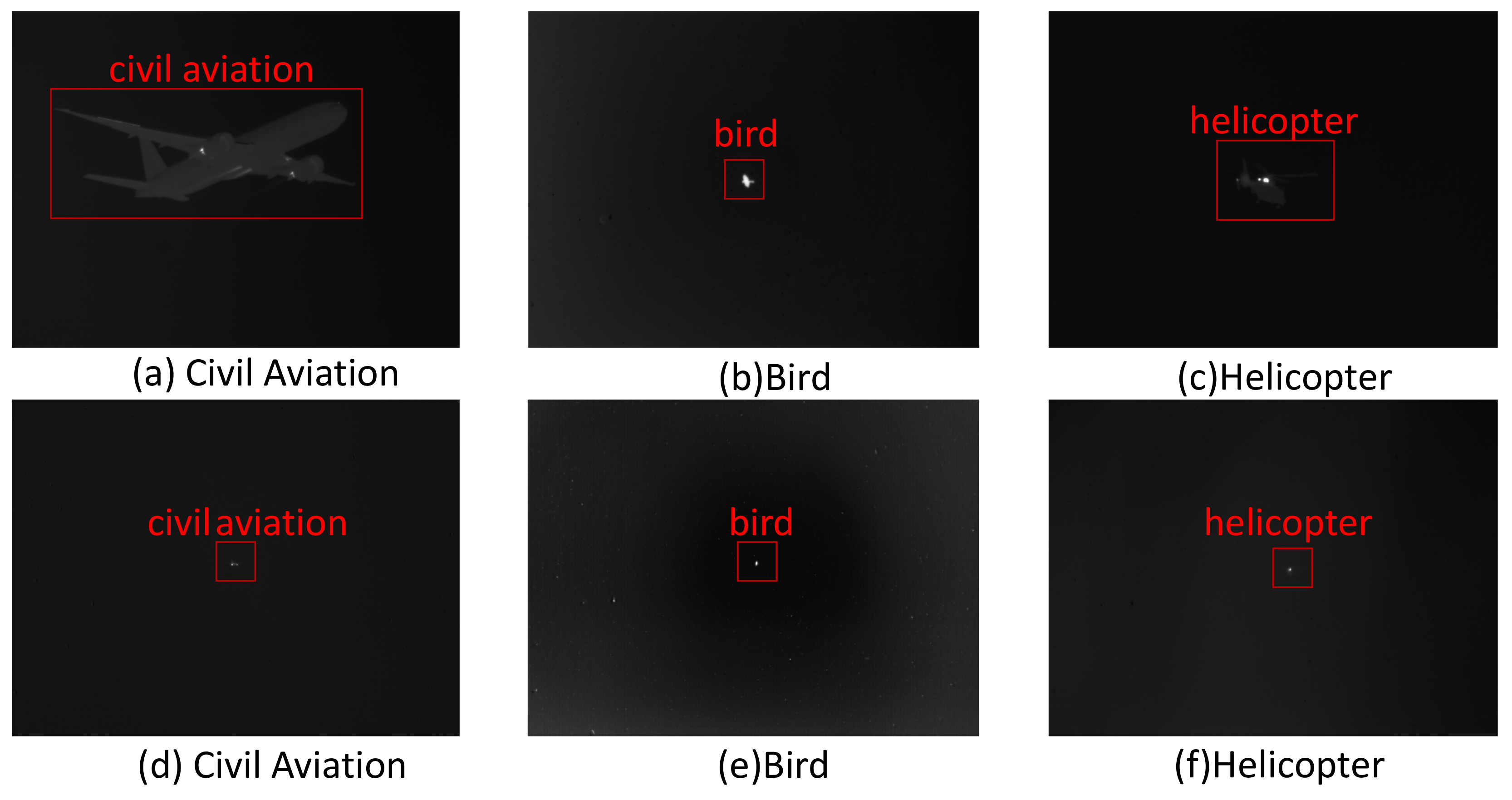
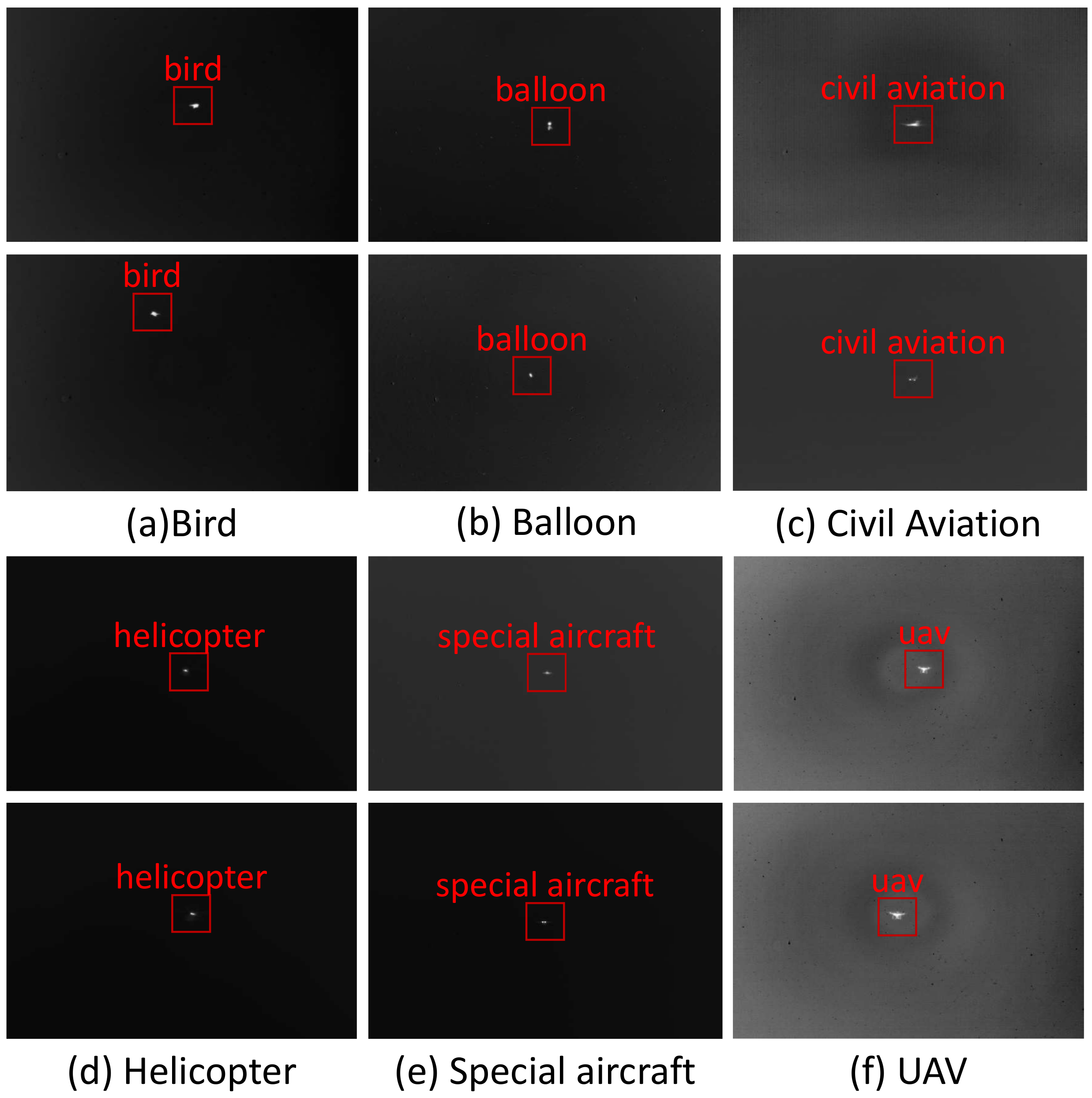
We invert the infrared images with a time length of 2 s into radiation characteristic samples with a sequential length of 200 using the infrared radiation measurement technique. We classify them using the ACGRU algorithm. Meanwhile, based on the classification results, we find a frame of the infrared image corresponding to the classification result, as shown in Figure 7. These images are infrared images before inversion at a specific moment in the time series samples correctly classified by the algorithm. From the images, it can be observed that our algorithm accurately classifies targets such as birds, balloons, and helicopters with insufficient morphological information. Our method provides a new approach for high-altitude object identification. The F1 score on the entire dataset reaches 93.9%, and the accuracy reaches 94.8%, further demonstrating the effectiveness of our method.

5.3. Ablation Experiment

In order to study the reliability of the ACGRU algorithm and the role of each component in the high-altitude flying object classification task, we conducted an ablation experiment. We gradually reduced the components on the complete ACGRU algorithm to observe their impact on performance, helping us understand the contributions of different components to the overall model performance, as well as their roles and necessity, and determine whether there are redundant parts. The experimental results are shown in Table 7, with a temporal length of 200 for the dataset. From the table, it can be seen that, after removing the Highway Network in the ACGRU algorithm, the accuracy decreased by 0.7% and the F1 score decreased by 1.1%. From the results, the inclusion of the Highway Network can increase the model’s attention to the original data, prevent the excessive abstraction of the data, and positively contribute to the model’s performance. Furthermore, when we removed the GRU-CNN component, the accuracy decreased by 3.4% and the F1 score decreased by 3.2%. This indicates that, for the ACGRU algorithm, both pathways are essential, and the GRU-CNN component is critically important to the algorithm’s performance. The F1 score of UAVs decreased the most severely after removing the components, reaching 6.4%. At the same time, the F1 scores of other classes generally decreased by around 3%. The F1 score only increases for helicopters, but the increase is not significant, and the amount of helicopter data are also relatively small. Therefore, we believe that the GRU-CNN component can compensate for the lack of long-term temporal correlation focus in the CNN-GRU component by extracting global temporal correlations. Finally, when we removed the attention module Senet, the accuracy decreased by 0.7% and the F1 score decreased by 1.2%. From the results, it can be seen that channel attention also has a positive effect on the model’s performance improvement. The reduction in each component led to a decline in algorithm performance, so we believe that each component of our algorithm plays a certain role, and the ACGRU algorithm we proposed is reliable and effective.

5.4. Experiments of ACGRU with Other Algorithms on Different Datasets

As we continue to incorporate more flying objects in our research, the overall radiation characteristic dataset will undergo changes, including the inclusion of a greater variety of datasets that differ from the six flying object datasets covered in this study. Therefore, we believe it is necessary to validate the proposed model’s ability to classify time-series data and its generalization in order to provide a reference for future research on classifying more high-altitude flying objects. Table 8 displays the accuracy performance of five models on a self-constructed infrared radiation characteristic dataset with a time series length of 200 and 17 datasets from UEA. Inception-Time is represented as IT. From the table, it can be seen that, among the five algorithms, ACGRU performs the best in our self-constructed dataset based on infrared radiation characteristics, with a 5.6% higher accuracy than FCN and a 3.3% higher accuracy than ConvTran. For the high-altitude flying object classification task, ACGRU is the most suitable algorithm among the five algorithms. At the same time, the ACGRU algorithm ranks first in the other 13 datasets, especially in cases where each category has a higher average training sample quantity. Except for the performance on the heartbeat dataset, which is not as good as ConvTran, ACGRU’s performance is better than the other models as the training volume increases. Furthermore, in the EigenWorms and EthanolConcentration datasets, when the time lengths are 17,984 and 1751, respectively, which is significantly higher than other datasets, ACGRU’s accuracy is noticeably higher than those of the other four algorithms. This indirectly validates ACGRU’s ability to focus on the long-term correlation information of time series data with longer time intervals. However, when the sample size is insufficient, ACGRU’s performance is not as good as the Transformer-based ConvTran algorithm. For example, in Cricket, despite the long time series length, the number of training samples is too small. Similarly, when both the number of training samples and time series length are insufficient, ACGRU’s performance is poor, as seen in the Libras dataset. Therefore, when performing different tasks, it is advisable to choose the appropriate algorithm based on the dataset conditions. In terms of high-altitude flying object classification tasks, ACGRU has the best performance, surpassing FCN by 5.6% and ConvTran by 3.3%.
In order to further analyze the performance of the ACGRU algorithm compared to the other four algorithms, we conducted significance tests. The Friedman test was used to determine whether the performance of the five algorithms was the same. A post hoc test, the Nemenyi test, was used to determine whether there were significant differences between the different algorithms [36]. The formula for conducting the Friedman test is described as follows:
χ F 2 = 12 N K ( K + 1 ) i = 1 K R i 2 K ( K + 1 ) 2 4
F F = ( N 1 ) · χ F 2 N · ( k 1 ) χ F 2
In this equation, χ F 2 represents the statistical value of the Friedman test that follows a χ 2 distribution, N represents the total number of data sets, K represents the number of algorithms, and R i 2 represents the average ranking value of the i-th algorithm. F F represents the statistical value of the Friedman test that follows an F-distribution. The Friedman test in Equation (30) is overly conservative, so we usually use the Friedman test that follows an F-distribution [36]. F F has k 1 and ( k 1 ) ( N 1 ) degrees of freedom. The critical values table can be found in any statistical textbook.
The formula describing the Nemenyi test is shown as Equation (32):
C D = q α 1 · K ( K + 1 ) 6 N
Among them, C D is the critical domain for the average rank difference of the algorithm. The value of q α 1 is shown in Table 9. α 1 represents the significance level, which indicates the probability of rejecting the null hypothesis. In this case, we set it to 0.05. When conducting the Nemenyi test, if the difference between the average values of the algorithms is greater than CD, we can conclude that there is a significant difference between these algorithms.
In Friedman’s test, the null hypothesis states that the performance of all algorithms is the same. According to Equations (30) and (31):
χ F 2 = 12 · 18 5 ( 5 + 1 ) ( 1 . 61 2 + 2 . 17 2 + 3 . 19 2 + 4 . 06 2 + 3 . 97 2 ) 5 ( 5 + 1 ) 2 4 = 33.99
F F = ( 18 1 ) · 33.99 18 · ( 5 1 ) 33.99 = 15.20
Using 5 algorithms and 18 datasets, F F is distributed according to the F distribution with (5 − 1) = 4 and (5 − 1) × (18 − 1) = 68 degrees of freedom. For α 1 = 0.05, the critical value of F(4, 68) is 2.51. Since 15.20 > 2.51, we reject the null hypothesis. There are differences among the 5 algorithms.
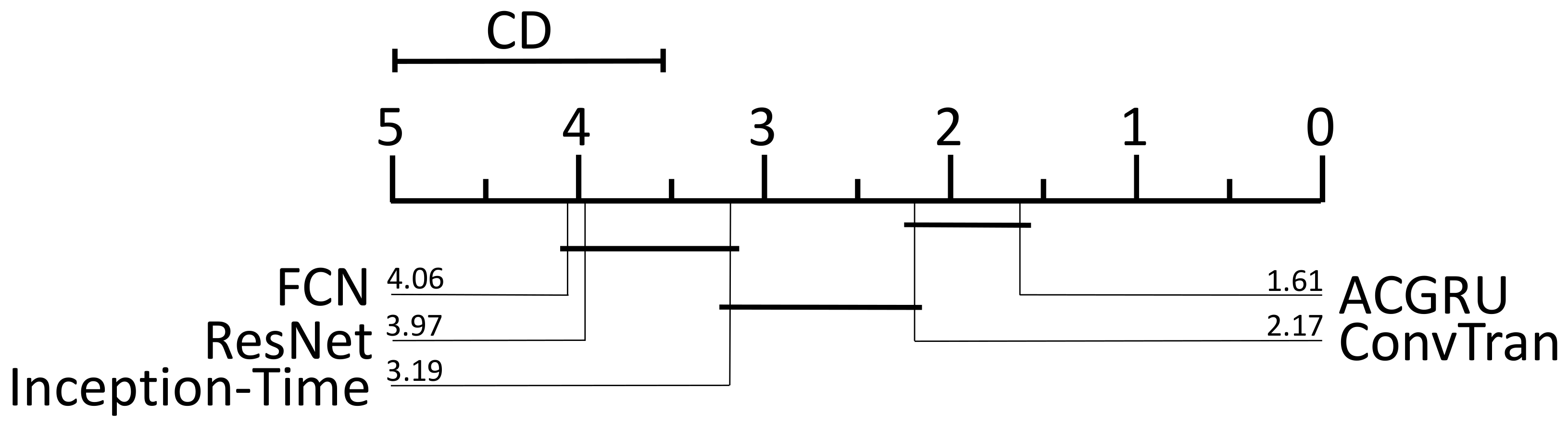
To further explore the differences between specific algorithms, we conducted the Nemenyi post hoc test. Based on Table 9, the value of q α 1 is 2.728, which means that CD is equal to 2.728 · 5 ( 5 + 1 ) 6 · 18 , with a value of 1.44. Therefore, ACGRU performs significantly better than Inception-Time (3.19 − 1.61 = 1.58 > 1.44), FCN (4.06 − 1.61 = 2.45 > 1.44), and ResNet (3.97 − 1.61 = 2.36 > 1.44). There is no significant difference between ACGRU and ConvTran (2.17 − 1.61 = 0.56 < 1.44). The significance differences between each classifier are shown in Figure 8, with the average rankings of each algorithm across all datasets plotted on the x axis.
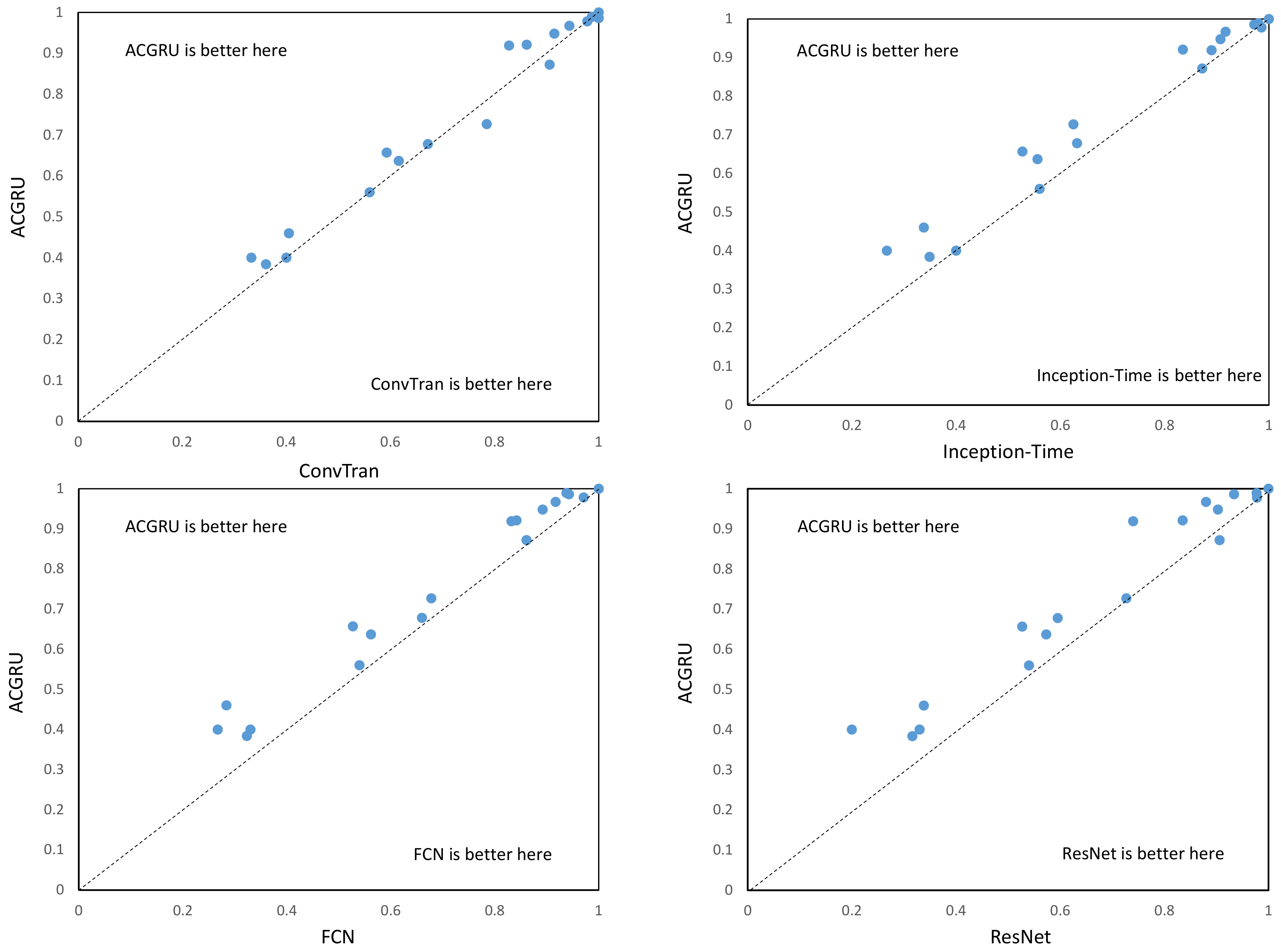
Based on the results of the significance analysis, we plotted the ACGRU algorithm separately with four other algorithms to further analyze the differences between ACGRU and these algorithms. The scatter plot shown in Figure 9 represents the accuracy of each classifier on the shared dataset, with each data point representing the accuracy difference between two classifiers. The larger the distance from the diagonal line, the greater the difference in accuracy between the two classifiers. Data points above the diagonal line indicate that the ACGRU algorithm outperforms the other models in terms of accuracy, while data points below the diagonal line indicate that the ACGRU algorithm is not as accurate as the other models. Although there is no significant difference between ACGRU and ConvTran, since ConvTran adopts Transformer technology that is fundamentally different from CNN and RNN, and Transformer is considered an advanced algorithm for processing sequential data, we consider the significant detection results between ACGRU and ConvTran to be acceptable. By observing Figure 8, we found that, for certain specific tasks, the accuracy of ACGRU is higher than that of ConvTran, especially for our high-altitude flying object classification task, where the accuracy of ACGRU is 3.3% higher than that of ConvTran. Thus, for the field of spatial governance, the ACGRU algorithm seems to be the more reasonable choice. On the other hand, ConvTran performs better than ACGRU in tasks with a smaller sample size and a longer-term dependency. From Figure 9, we can see that, for the majority of the datasets, ACGRU outperforms Inception-Time, FCN, and ResNet algorithms, indicating that ACGRU has a clear advantage over them.
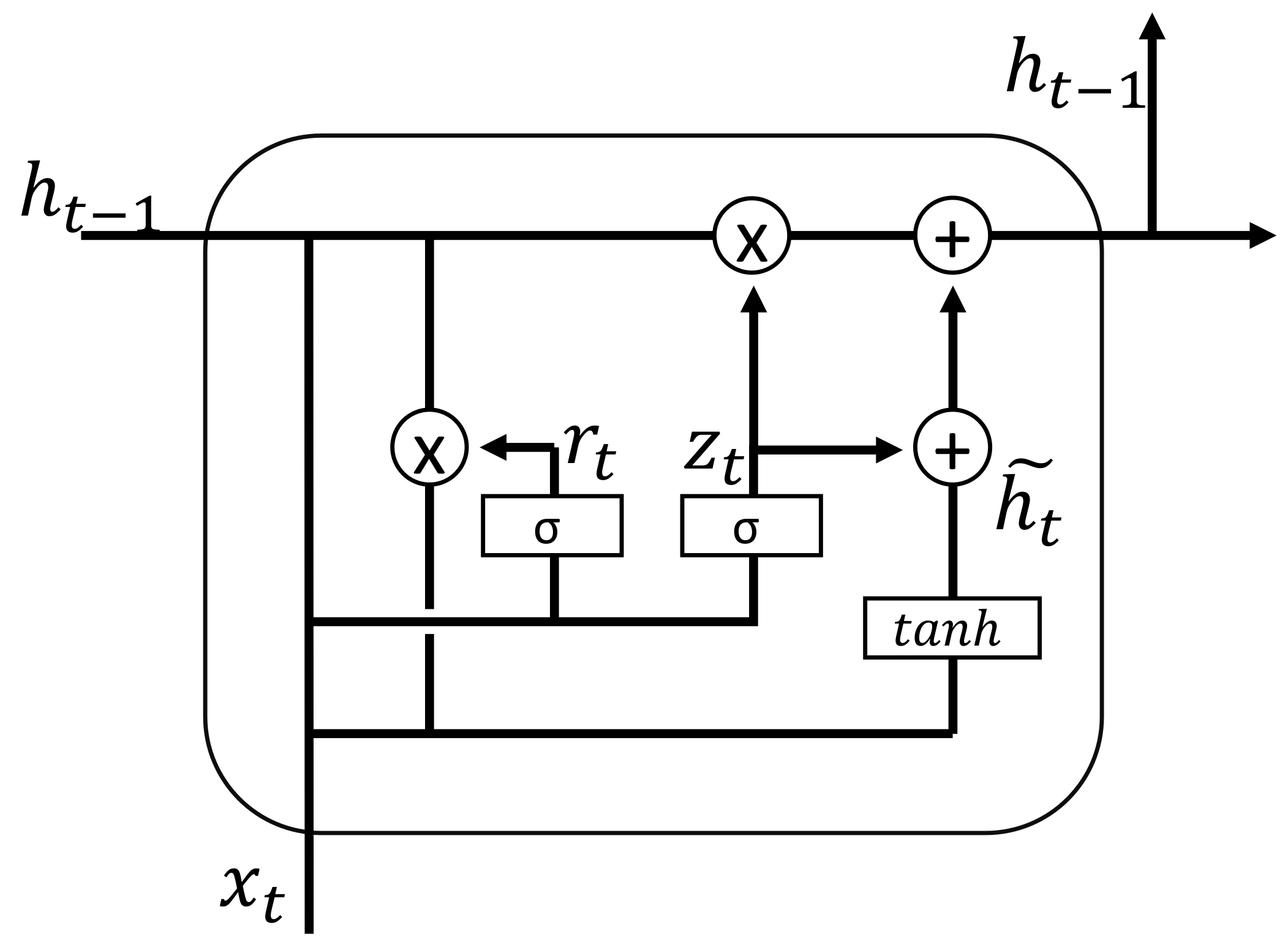
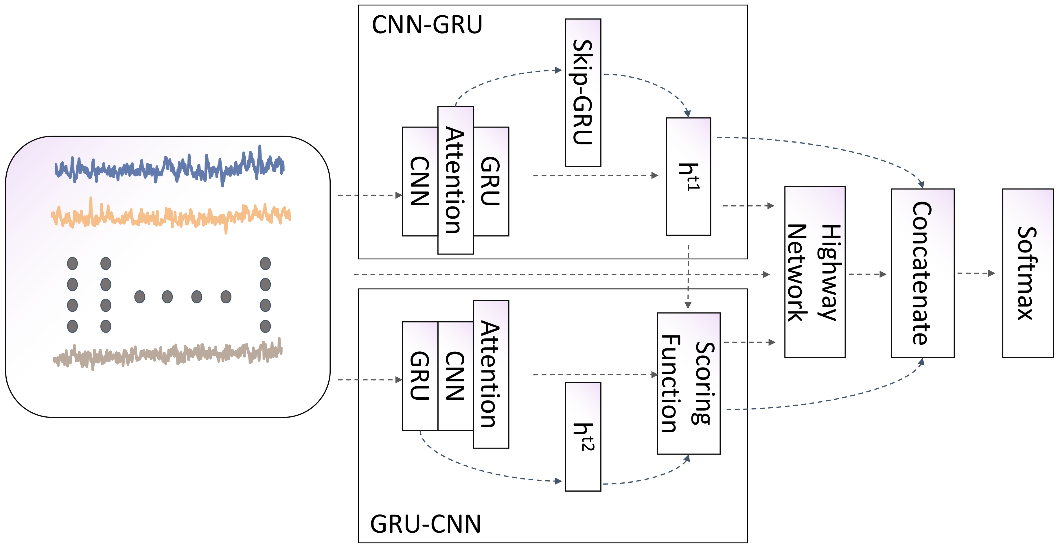
The ACGRU algorithm combines the attention mechanism and constructs three pathways: CNN-GRU, GRU-CNN, and Highway Network, fully leveraging the advantages of convolutional neural networks (CNNs) and recurrent neural networks (RNNs). CNN is capable of extracting local and global temporal features, while RNN captures the temporal relationships of time series. The synergistic effect of the CNN-GRU and GRU-CNN components further enhances the information extraction capacity of the original data, while the Highway Network alleviates the gradient vanishing problem and prevents the excessive abstraction of data. Compared to the FCN and ResNet algorithms, ACGRU can preserve more temporal information because GRU can process and memorize features at each time step. The ACGRU model reorganizes the temporal data, draws inspiration from the temporal data convolution idea of Inception-Time, but incorporates the exchange and combination of GRU and the attention mechanism to more effectively extract temporal information. Through significance analysis, the ACGRU algorithm significantly outperforms Inception-Time, FCN, and ResNet. Although there is no significant difference compared to ConvTran, both algorithms have their own advantages. ConvTran performs better in handling small sample datasets, while ACGRU excels in handling our self-made high-altitude flying object classification dataset. Therefore, we believe that ACGRU is suitable for high-altitude flying object classification tasks, as it can effectively model the long-term dependencies and local features in time series data, improve the modeling ability of time series data, and demonstrate a certain level of generalization. This will help in the subsequent addition of more high-altitude flying objects and the construction of more complex infrared radiation datasets to achieve accurate classification.

6. Conclusions

In the study of the classification of high-altitude flying objects, it is difficult to classify them based solely on the shape and contour of the flying objects due to altitude issues. In this study, high-altitude flying objects were captured using a long-wave infrared camera, and the radiation characteristics were measured to calculate the inverted radiation characteristic data, obtaining multidimensional sequential data. To expand the dataset, data noise simulation was performed. To investigate the optimal time required for classification, five datasets with different time sequence lengths were prepared. Subsequently, an attention-based convolutional neural network (CNN) and gated recurrent unit (GRU) algorithm, named ACGRU, was proposed for the classification of high-altitude flying objects. The ACGRU algorithm computes the radiation dataset through three paths: CNN-GRU, GRU-CNN, and the Highway Network. The computed results are then fused for the classification experiment. To verify the effects of the three paths on classification results, an ablation experiment was conducted to further validate the effectiveness of ACGRU. Finally, considering that the addition of more flying objects will result in changes in the dataset variance, a model generalization study was carried out. Comparative experiments and significance analysis were conducted on our self-built dataset and 17 publicly available datasets from UEA, compared with our four other algorithms. The experimental results indicate that, considering both speed and accuracy, the radiation characteristic dataset with a time sequence length of 200 is most suitable for flying object classification. The corresponding imaging time of the long-wave infrared camera is 2 s. The ACGRU algorithm achieves an accuracy of 94.8% and an F1 score of 93.9% in the classification of high-altitude flying objects. The ablation experiment results show that the classification accuracy of the complete ACGRU algorithm is improved by 4.8% compared to the single-path CNN-GRU. Among the 17 publicly available datasets, our algorithm significantly outperforms Inception-Time, FCN, and ResNet, but shows no significant difference from ConvTran. Compared to ConvTran, when facing an insufficient data volume and insufficient time sequence lengths for multidimensional time series data, ACGRU performs weaker: when facing sufficient data volume and sufficient time sequence lengths, ACGRU performs better. The classification accuracy of ACGRU in the radiation characteristic dataset is 3.3% higher than that of ConvTran. For our high-altitude flying object classification task, the ACGRU algorithm is the most suitable algorithm, which has certain practical value in applications such as air defense. However, our method still has some limitations. The current approach cannot manage multiple flying objects simultaneously. In addition, the infrared feature inversion system and the target classification algorithm system are operated independently. Therefore, in the future, we will improve the algorithm by incorporating target tracking and multi-object recognition techniques. We will integrate image acquisition inversion with radiometric classification to achieve an end-to-end process of image acquisition and classification. This will enable the system to handle multiple flying objects at high altitudes and enhance its comprehensive target classification capability. At the same time, we will expand the types of radiometric datasets and strengthen the model’s ability to classify more high-altitude flying objects.

Author Contributions

Conceptualization, D.D.; methodology, D.D. and L.C.; software, D.D.; validation, Y.L., Y.W. and Z.W.; formal analysis, Y.L., Y.W. and Z.W.; investigation, D.D., Y.L., Y.W. and Z.W.; resources, D.D., Y.L. and Y.W.; data curation, Y.L. and Y.W.; writing—original draft preparation, D.D., Y.L., Y.W. and Z.W.; writing—review and editing, D.D. and L.C.; supervision, D.D., L.C. and Y.L.; project administration, D.D.; funding acquisition, L.C. All authors have read and agreed to the published version of the manuscript.

Funding

This research received no external funding.

Data Availability Statement

Not applicable.

Conflicts of Interest

The authors declare no conflict of interest.

References

  1. Stancic, I.; Veic, L.; Music, J.; Grujic, T. Classification of Low-Resolution Flying Objects in Videos Using the Machine Learning Approach. Adv. Electr. Comput. Eng. 2022, 22, 45–52. [Google Scholar] [CrossRef]
  2. Deng, L.; Zhang, J.; Xu, G.; Zhu, H. Infrared small target detection via adaptive M-estimator ring top-hat transformation. Pattern Recognit. 2021, 112, 107729. [Google Scholar] [CrossRef]
  3. Zhang, T.; Peng, Z.; Wu, H.; He, Y.; Li, C.; Yang, C. Infrared small target detection via self-regularized weighted sparse model. Neurocomputing 2021, 420, 124–148. [Google Scholar] [CrossRef]
  4. Ju, M.; Luo, J.; Liu, G.; Luo, H. ISTDet: An efficient end-to-end neural network for infrared small target detection. Infrared Phys. Technol. 2021, 114, 103659. [Google Scholar] [CrossRef]
  5. Li, B.; Xiao, C.; Wang, L.; Wang, Y.; Lin, Z.; Li, M.; An, W.; Guo, Y. Dense Nested Attention Network for Infrared Small Target Detection. IEEE Trans. Image Process. 2023, 32, 1745–1758. [Google Scholar] [CrossRef] [PubMed]
  6. Deng, X.; Wang, Y.; Han, G.; Xue, T. Research on a measurement method for middle-infrared radiation characteristics of aircraft. Machines 2022, 10, 44. [Google Scholar] [CrossRef]
  7. Wang, W.; Cheng, J.; Si, W. Small-target judging method based on the effective image pixels for measuring infrared radiation characteristics. Appl. Opt. 2020, 59, 3124–3131. [Google Scholar] [CrossRef] [PubMed]
  8. Kou, T.; Zhou, Z.; Liu, H.; Yang, Z. Correlation between infrared radiation characteristic signals and target maneuvering modes. Acta Opt. Sin. 2018, 38, 37–45. [Google Scholar]
  9. Chen, Y.; Wang, D.; Shao, M. Study on the infrared radiation characteristics of the sky background. In Proceedings of the AOPC 2015: Telescope and Space Optical Instrumentation, Beijing, China, 6–7 June 2015; SPIE: Cergy, France, 2015; Volume 9678, pp. 89–93. [Google Scholar]
  10. Insua, D.R.; Ruggeri, F.; Soyer, R.; Wilson, S. Advances in Bayesian decision making in reliability. Eur. J. Oper. Res. 2020, 282, 1–18. [Google Scholar] [CrossRef]
  11. Zhang, Z. Introduction to machine learning: K-nearest neighbors. Ann. Transl. Med. 2016, 4, 218. [Google Scholar] [CrossRef]
  12. Noble, W.S. What is a support vector machine? Nat. Biotechnol. 2006, 24, 1565–1567. [Google Scholar] [CrossRef]
  13. Gu, J.; Wang, Z.; Kuen, J.; Ma, L.; Shahroudy, A.; Shuai, B.; Liu, T.; Wang, X.; Wang, G.; Cai, J.; et al. Recent advances in convolutional neural networks. Pattern Recognit. 2018, 77, 354–377. [Google Scholar] [CrossRef]
  14. Chung, J.; Gulcehre, C.; Cho, K.H.; Bengio, Y. Empirical evaluation of gated recurrent neural networks on sequence modeling. arXiv 2014, arXiv:1412.3555. [Google Scholar]
  15. Schmidhuber, J. Deep learning in neural networks: An overview. Neural Netw. 2015, 61, 85–117. [Google Scholar] [CrossRef] [PubMed]
  16. Zhu, K.; Yin, M.; Zhu, D.; Zhang, X.; Gao, C.; Jiang, J. SCGRU: A general approach for identifying multiple classes of self-admitted technical debt with text generation oversampling. J. Syst. Softw. 2023, 195, 111514. [Google Scholar] [CrossRef]
  17. Cai, J.; Zhang, K.; Jiang, H. Power Quality Disturbance Classification Based on Parallel Fusion of CNN and GRU. Energies 2023, 16, 4029. [Google Scholar] [CrossRef]
  18. Yadav, H.; Shah, P.; Gandhi, N.; Vyas, T.; Nair, A.; Desai, S.; Gohil, L.; Tanwar, S.; Sharma, R.; Marina, V.; et al. CNN and Bidirectional GRU-Based Heartbeat Sound Classification Architecture for Elderly People. Mathematics 2023, 11, 1365. [Google Scholar] [CrossRef]
  19. Kim, A.R.; Kim, H.S.; Kang, C.H.; Kim, S.Y. The design of the 1D CNN–GRU network based on the RCS for classification of multiclass missiles. Remote Sens. 2023, 15, 577. [Google Scholar] [CrossRef]
  20. Prokhorov, A.V.; Hanssen, L.M.; Mekhontsev, S.N. Calculation of the radiation characteristics of blackbody radiation sources. Exp. Methods Phys. Sci. 2009, 42, 181–240. [Google Scholar]
  21. Yuan, H.; Wang, X.; Guo, B.; Li, K.; Zhang, W.G. Modeling of the Mid-wave Infrared Radiation Characteristics of the Sea surface based on Measured Data. Infrared Phys. Technol. 2018, 93, 1–8. [Google Scholar] [CrossRef]
  22. Bagnall, A.; Dau, H.A.; Lines, J.; Flynn, M.; Large, J.; Bostrom, A.; Southam, P.; Keog, E. The UEA Multivariate Time Series Classification Archive, 2018. arXiv 2018, arXiv:1811.00075. [Google Scholar]
  23. Mahulikar, S.P.; Sonawane, H.R.; Rao, G.A. Infrared signature studies of aerospace vehicles. Prog. Aerosp. Sci. 2007, 43, 218–245. [Google Scholar] [CrossRef]
  24. Ludwig, C.B.; Malkmus, W.; Walker, J.; Slack, M.; Reed, R. The standard infrared radiation model. AIAA Paper 1981, 81, 1051. [Google Scholar]
  25. Choudhury, S.L.; Paul, R.K. A new approach to the generalization of Planck’s law of black-body radiation. Ann. Phys. 2018, 395, 317–325. [Google Scholar] [CrossRef]
  26. Niu, Z.; Zhong, G.; Yu, H. A review on the attention mechanism of deep learning. Neurocomputing 2021, 452, 48–62. [Google Scholar] [CrossRef]
  27. Woo, S.; Park, J.; Lee, J.Y.; Kweon, I.S. Cbam: Convolutional block attention module. In Proceedings of the European Conference on Computer Vision (ECCV) 2018, Munich, Germany, 8–14 September 2018; pp. 3–19. [Google Scholar]
  28. Hu, J.; Shen, L.; Sun, G. Squeeze-and-excitation networks. In Proceedings of the IEEE Conference on Computer Vision and Pattern Recognition (CVPR) 2018, Salt Lake City, UT, USA, 18–22 June 2018; pp. 7132–7141. [Google Scholar]
  29. LeCun, Y.; Bengio, Y.; Hinton, G. Deep learning. Nature 2015, 521, 436–444. [Google Scholar] [CrossRef] [PubMed]
  30. Zhang, A.; Lipton, Z.C.; Li, M.; Smola, A.J. Dive Into Deep Learning. arXiv 2021, arXiv:2106.11342. [Google Scholar]
  31. Glorot, X.; Bengio, Y. Understanding the difficulty of training deep feedforward neural networks. In Proceedings of the Thirteenth International Conference on Artificial Intelligence and Statistics—JMLR Workshop and Conference Proceedings, Sardinia, Italy, 13–15 May 2010; pp. 249–256. [Google Scholar]
  32. Srivastava, R.K.; Greff, K.; Schmidhuber, J. Highway networks. arXiv 2015, arXiv:1505.00387. [Google Scholar]
  33. Ismail Fawaz, H.; Forestier, G.; Weber, J.; Idoumghar, L.; Muller, P.A. Deep Learning for Time Series Classification: A Review. Data Min. Knowl. Discov. 2019, 33, 917–963. [Google Scholar] [CrossRef]
  34. Ruiz, A.P.; Flynn, M.; Large, J.; Middlehurst, M.; Bagnall, A. The Great Multivariate Time Series Classification Bake Off: A Review and Experimental Evaluation of Recent Algorithmic Advances. Data Min. Knowl. Discov. 2021, 35, 401–449. [Google Scholar] [CrossRef]
  35. Foumani, N.M.; Tan, C.W.; Webb, G.I.; Salehi, M. Improving Position Encoding of Transformers for Multivariate Time Series Classification. arXiv 2023, arXiv:2305.16642. [Google Scholar] [CrossRef]
  36. Demšar, J. Statistical comparisons of classifiers over multiple data sets. J. Mach. Learn. Res. 2006, 7, 1–30. [Google Scholar]
Figure 2. Illustration of a long-wave infrared camera.
Remotesensing 15 04985 g002
Figure 3. Graphical representation of the infrared image of high-altitude flying objects.
Remotesensing 15 04985 g003
Figure 4. Radiation feature data, with the horizontal axis representing the frame number of the video, and the vertical axis representing the radiation intensity.
Remotesensing 15 04985 g004
Figure 5. Radiation characteristic data with four types of noise added.
Remotesensing 15 04985 g005
Figure 6. Graphical representation of the ACGRU structure.
Remotesensing 15 04985 g006
Figure 7. The infrared image corresponding to a certain temporal sequence in the classification result.
Remotesensing 15 04985 g007
Figure 8. Comparison of all classifiers against each other with the Nemenyi test. Groups of classifiers that are not significantly different are connected.
Remotesensing 15 04985 g008
Figure 9. Scatter plots of pairwise comparison of all models against ACGRU.
Remotesensing 15 04985 g009
Table 1. CNN-GRU component and its related parameters.
LayerOutput MatrixOutput ShapeAttribute
Conv1H ( N o n e , 100 , 200 , 1 ) C o n v 2 d ( 1 , 100 , k e r n e l _ s i z e = ( 3 , 8 ) , s t r i d e = ( 1 , 1 ) , p a d d i n g = ( 1 , 0 ) )
Senet H s ( N o n e , 100 , 200 , 1 )
Squeeze ( N o n e , 100 , 200 )
Permute ( 200 , N o n e , 100 )
GRU H t 1 g ( N o n e , 100 ) G R U ( i n p u t _ s i z e = 100 , h i d d e n _ s i z e = 100 )
Skip-GRU H t 1 s ( N o n e , 100 ) G R U ( i n p u t _ s i z e = 100 , h i d d e n _ s i z e = 100 )
Concatenate ( N o n e , 200 )
Linear H t 1 ( N o n e , 8 ) L i n e a r ( i n _ f e a t u r e s = 200 , o u t _ f e a t u r e s = 8 , b i a s = T r u e )
Table 2. GRU-CNN component and its related parameters.
LayerOutput MatrixOutput ShapeAttribute
GRU H t 2 ( 1 , N o n e , 12 ) G R U ( i n p u t _ s i z e = 8 , h i d d e n _ s i z e = 12 , n u m _ l a y e r s = 3 )
GRU H t × s ( 200 , N o n e , 12 ) G R U ( i n p u t _ s i z e = 8 , h i d d e n _ s i z e = 12 , n u m _ l a y e r s = 3 )
Permute H t 2 ( N o n e , 1 , 12 )
Permute H t × s ( N o n e , 200 , 12 )
Unsqueeze H t × s ( N o n e , 1 , 200 , 12 )
Conv1 ( N o n e , 100 , 200 , 1 ) C o n v 2 d ( 1 , 100 , k e r n e l _ s i z e = ( 3 , 12 ) , s t r i d e = ( 1 , 1 ) , p a d d i n g = ( 1 , 0 ) )
Senet H k × t × 1 ( N o n e , 100 , 200 , 1 )
Squeeze H k × t ( N o n e , 100 , 200 )
Scoring function h t s ( N o n e , 8 , 1 )
Squeeze H t s ( N o n e , 8 )
Table 3. Highway Network component and its related parameters.
LayerOutput MatrixOutput ShapeAttribute
Data processingDP(X) ( N o n e , 8 ) L i n e a r ( i n _ f e a t u r e s = 16 , o u t _ f e a t u r e s = 8 , b i a s = T r u e )
ReshapeX ( N o n e , 1600 )
LinearX ( N o n e , 8 ) L i n e a r ( i n _ f e a t u r e s = 1600 , o u t _ f e a t u r e s = 8 , b i a s = T r u e )
Highway network H ( X ) ( N o n e , 8 )
Table 4. The quantities of different types of targets IN training and test sets in the 5 radiation characteristic datasets.
Radiation Characteristic DataTraining Set of Length 50Test Set of Length 50Training Set of Length 100Test Set of Length 100Training Set of Length 200Test Set of Length 200Training Set of Length 300Test Set of Length 300Training Set of Length 400Test Set of Length 400
Bird14,323358371611792358089623865981789448
Balloon14,303357571511788357589423835961787447
Civil aviation17124288562144281072857121454
Helicopter2485623124231262115641410431078
Special aircraft8530213142651065213253314213561065267
Small UAVs4096102420485121024256682170512128
All45,44911,36422,723568311,36028427571189556771422
Table 5. The classification results of the ACGRU algorithm for 5 radiation characteristic datasets.
Radiation Characteristic DataTest Set of Length 50Test Set of Length 100Test Set of Length 200Test Set of Length 300Test Set of Length 400
Rec of bird0.9460.9600.9640.9580.960
Rec of balloon0.9310.9390.9420.9530.946
Rec of civil aviation0.9460.9490.9440.9440.926
Rec of helicopter0.8970.9010.9040.9040.897
Rec of special aircraft0.9270.9430.9590.9520.963
Rec of UAVs0.9110.9180.9220.9240.914
Acc of all0.9320.9430.9480.9490.947
Table 6. The classification results of the ACGRU algorithm for high-altitude flying objects.
Radiation Characteristic DataTrain SetTest SetLengthCorrectPrecisionRecallF1 ScoreAcc
Bird35808962008640.9610.9640.962-
balloon35758942008420.9360.9420.939-
Civil aviation4281072001010.8940.9440.918-
Helicopter6211562001410.9340.9040.919-
Special aircraft21325332005110.9640.9590.961-
UAVs10242562002360.9480.9220.935-
All11,360284220026950.9400.9390.9390.948
Table 7. Results of ablation experiment.
Radiation Characteristic DataCNN-GRUCNN-GRU + SenetCNN-GRU + GRU-CNN + SenetACGUR
F1 of bird0.9150.9240.9520.962
F1 of balloon0.9110.9130.940.939
F1 of civil aviation0.8730.870.9080.918
F1 of helicopter0.8550.8940.8820.919
F1 of special aircraft0.9000.8940.9460.961
F1 of UAVs0.8520.8780.9420.935
F1 of all0.8840.8960.9280.939
Acc of all0.9000.9070.9410.948
Table 8. The accuracy and average ranking of the five models on 18 multivariate time series datasets.
DatasetAvg TrainLengthACGRUConvTranITFCNResNet
FaceDetection2945620.6780.6720.6320.660.595
PenDigits75080.9890.9870.980.9380.977
LSST176360.6370.6160.5560.5620.573
FingerMovement158500.560.560.560.540.54
Heartbeat1024050.7270.7850.6250.6780.727
EthanolConcentration6617510.3840.3610.3490.3230.316
HandMovement404000.460.4050.3380.2840.338
PEMS-SF391440.9190.8280.890.8320.74
RacketSports38300.9210.8620.8350.8420.835
Epilepsy352070.9780.9780.9860.9710.978
NATOPS30510.9670.9440.9170.9170.88
EigenWorms2617,9840.6570.5930.5270.5270.527
Libras12450.8720.9060.8720.8610.906
BasicMotions1010011111
Cricket911970.98610.9720.9430.934
AtrialFibrillation56400.40.40.2670.2670.2
StandWalkJump425000.40.3330.40.330.33
MyData18952000.9480.9150.9070.8920.903
Win 146412
Average rank 1.612.173.194.063.97
Table 9. Critical values for the two-tailed Nemenyi test [36].
Classifiers2345678910
q 0.05 1.9602.3442.5692.7282.8502.9493.0313.1023.164
q 0.10 1.6452.0522.2912.4592.5892.6932.7802.8552.920
Disclaimer/Publisher’s Note: The statements, opinions and data contained in all publications are solely those of the individual author(s) and contributor(s) and not of MDPI and/or the editor(s). MDPI and/or the editor(s) disclaim responsibility for any injury to people or property resulting from any ideas, methods, instructions or products referred to in the content.

