Evaluating the Uncertainty in Coherence-Change-Detection-Based Maps of Torrential Sediment Transport in Arid Environments

Abstract

InSAR coherence-change detection (CCD) is a promising remote sensing technique that is able to map areas affected by torrential sediment transport triggered by flash floods in arid environments. CCD maps the changes in the interferometric coherence between synthetic aperture radar images (InSAR coherence), a parameter that measures the stability of the radar signal between two different SAR images, i.e., data acquisitions. In arid environments, such changes are mainly due to changes in the surface. However, the residual effect of other factors on the InSAR coherence cannot be completely excluded. Therefore, CCD-based maps contain the uncertainty of whether the detected changes are actual changes in the observed surface or just errors related to those residual effects. Thus, in this paper, the results of four CCD mapping methods, with different degrees of complexity and sensitivity to the different factors affecting the InSAR coherence, are compared in order to evaluate the existence of the errors and their importance. The obtained CCD maps are also compared with changes in satellite optical images and a field campaign. The results lead to the conclusion that CCD maps are reliable in the identification of the zones affected by sediment transport, although the precision in the delimitation of the affected area remains an open issue. However, highly rugged relief areas still require a thorough analysis of the results in order to discard the geometric effects related to the perpendicular baseline.

1. Introduction

In arid environments, the small annual amount of precipitation is typically concentrated in a few rare events that often cause flash floods [1,2,3,4,5]. These floods drag a significant amount of sediment that causes serious damage to the delicate ecosystems of these environments and human settlements [2,3,4,6,7]. In addition, the torrential sediment transport in arid environments is characterised by a greater proportion of coarse-grained sediments (gravel, cobbles, and boulders) than in areas with a more humid climate, which makes flash floods particularly destructive [3,6,7,8]. One of the most common protective measures for urban areas against flash floods is the construction of sediment-detention basins. The sediments carried by water are retained in these structures during the flood, after which they must be removed by mechanical means to free the storage capacity for future events [7]. In order to design a sediment-detention basin, it is necessary to know the volume of sediments to be retained, which, in turn, requires determining the sediment-contributing basin. These areas of contribution are often remote and extensive, so their determination is a difficult task. Fortunately, InSAR coherence-change detection (CCD) is emerging as a potential solution.

CCD is a promising technique for remotely mapping phenomena that disturb the ground surface over large and inaccessible areas, with a greater sensitivity than optical techniques and in an easier and cheaper way than field campaigns [1,4,9,10,11]. It consists of tracking the changes in the interferometric coherence between synthetic aperture radar (SAR) images. The InSAR coherence is a measure of the stability of the radar signal between two different SAR images, i.e., data acquisitions [12,13,14]. Several factors determine this stability: (i) the perpendicular baseline, i.e., the distance between the position of the radar during the different data acquisitions in the direction perpendicular to the radar line of sight; (ii) the temporal baseline, i.e., the time lapse between radar images; (iii) changes in soil moisture; and (iv) changes in the observed surface [1,15,16,17]. The basis of CCD is that if one factor prevails under certain conditions, the changes in InSAR coherence reflect the evolution of this factor.

The main difficulty of CCD is that, in reality, even if changes in the observed surface may dominate over the other factors, they will never be the only factor affecting the InSAR coherence. Therefore, because of the residual contributions of these other factors, there is uncertainty as to whether the detected changes are actual changes in the observed surface or just errors [1]. The main sources of uncertainty are the perpendicular baseline [15,17] and changes in soil moisture [18,19]. For instance, when mapping the area affected by torrential sediment-transport events (erosion and sedimentation) caused by flash floods, the effect of the perpendicular baseline, which is directly related to the local slope of the surface, is particularly distorting because it is maximal in rugged areas, which are precisely the areas that are the most susceptible to sediment transport. Thus, we might wonder whether what we “see” with InSAR coherence data are the effects caused by the perpendicular baseline or actual erosion or sedimentation along the gully.

There are basically two ways of trying to distinguish actual changes in the observed surface from other factors affecting the InSAR coherence: (i) modelling the components of the coherence or (ii) directly correlating the changes in the coherence with other observations (for example, coincidence in time with meteorological events or correspondence in space with lithology or land cover, among many others). In the first case, the idea is that, once each component of the coherence (or, equivalently, of the so-called decorrelation, which is the loss of coherence) is modelled, all the contributions not related to surface changes can be removed so that the remaining changes in InSAR coherence reproduce actual changes in the observed surface. There are two kinds of models: analytical models [20,21] and empirical models [11,16,19,22,23,24]. The former are based on the physics of the measurement, i.e., of InSAR, while the latter are based on empirical, often statistical correlations. While, in theory, analytical models should provide the most accurate results, in practice, they require simplifications of reality that make it difficult to find the right conditions for calibrating the several parameters that they often include. This double complexity—several parameters to calibrate and the difficulty in finding the right conditions to calibrate them—has limited their development [24]. In contrast, empirical models, which by their nature already incorporate the “imperfections” of reality, tend to perform better despite being generally simpler. This is why there are more examples of empirical models than of analytical models in the literature. Nevertheless, the construction of a robust empirical model requires time series of both SAR data and the data used for the correlation to be long enough to be statistically representative, which is a major challenge when studying the effects of flash floods in arid environments. Finally, the most abundant case in the literature is still the direct correlation with other data, observations or prior knowledge [1,4,9,10,15,25,26]. However, although previous studies confirm the ability of CCD to detect surface changes [27], none of the mentioned approaches have yet resolved how to map surface changes using CCD with certainty [1].

Thus, in this paper, we propose several mapping methods for torrential sediment transport events in arid environments based on CCD, each one with a different degree of complexity and a different sensitivity to each component of the decorrelation, aiming to reduce the uncertainty in the CCD mapping by comparing their results and assessing their degree of coincidence or divergence.

This paper is organised in five sections and two appendices. After this introduction, Section 2 presents (i) the study area; (ii) the data used in this research; (iii) the methods used, first, to map the area affected by torrential sediment transport events and, second, to compare and discuss the results; and (iv) the followed procedure. Section 3 presents the results, which are analysed and discussed in context with the literature in Section 4. Finally, Section 5 closes the paper with the conclusions and possible future lines of research.

2. Materials and Methods

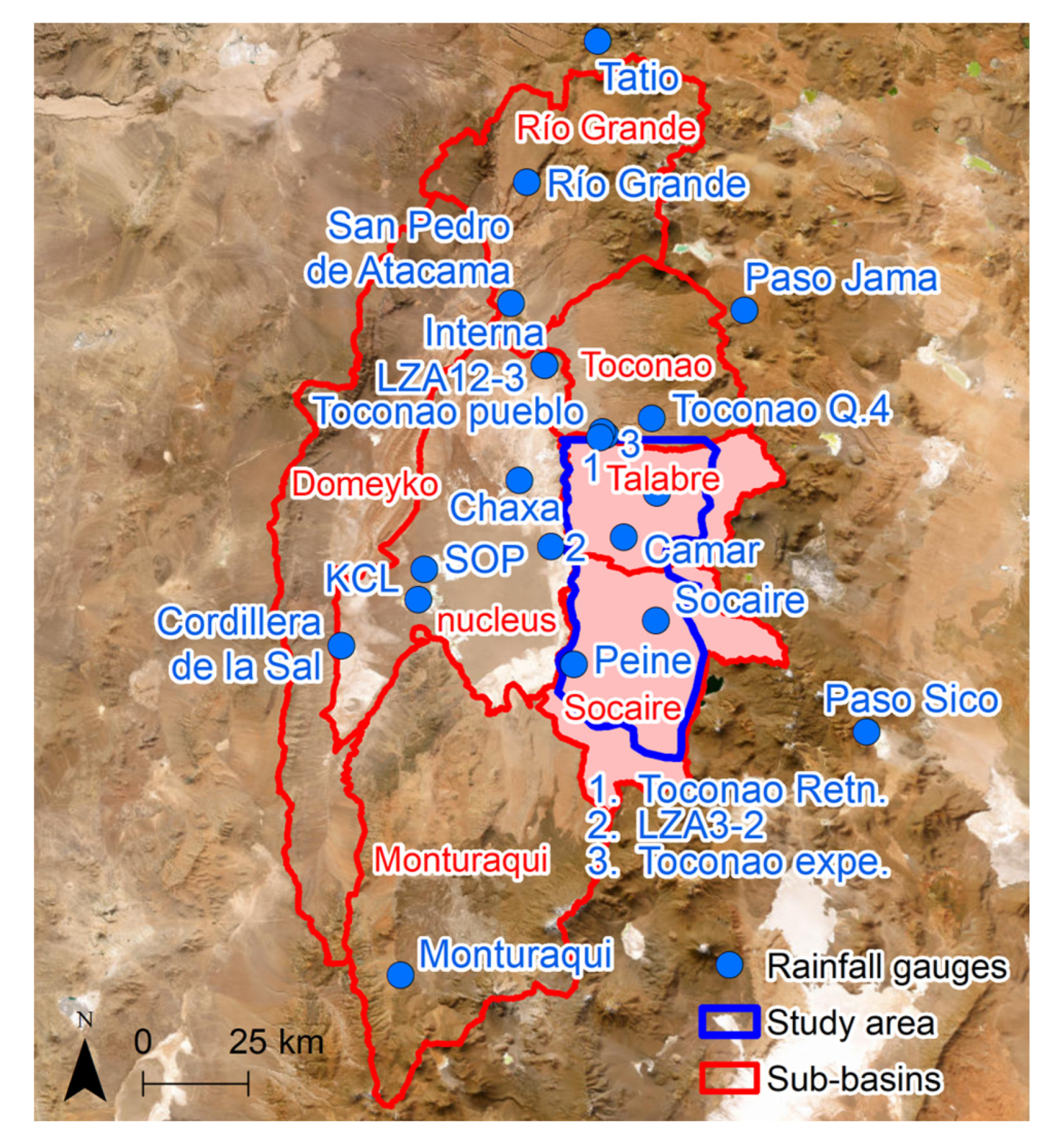
2.1. Study Area

The analysis of the reliability of the CCD-based maps of the area affected by torrential sediment transport events in arid environments was performed in a study area within the Salar de Atacama Basin, Chile. The Salar de Atacama Basin is an endorheic basin located in northern Chile between 22.5° and 23.5° south latitude and 67.5° and 68.5° west longitude in the Antofagasta region (Figure 1a). The basin is enclosed by the Western Central Andean Range to the east, which is oriented N–S and reaches 6100 m.a.s.l. (metres above sea level); the Domeyko Range to the west, a secondary Andean range that reaches 4000 m.a.s.l. and is oriented NNE–SSW, merging the Western Central Andean Range to the north and closing the basin; and the Cordón de Lila to the south, a 3200 m.a.s.l. high mountain range (Figure 1b). In total, the basin extends over some 17,000 km^2, and the salt pan in the nucleus covers some 3000 km² at an altitude of 2300 m.a.s.l.

In its nucleus, Salar de Atacama hosts 40% of the world’s reserves of lithium and large amounts of boron and potassium, among several other salts [28], as well as numerous lagoons and wetlands along its eastern marginal zone, several of which are classified as UNESCO-Ramsar sites that represent precious and highly sensitive ecological habitats for several migratory and endemic species of flora and fauna [29].

Most of the annual precipitation in the Salar de Atacama Basin (87%) is brought by the humid air masses dragged by the easterly winds from the Atlantic Ocean through the Amazonia and the Gran Chaco to the Andean Range during the austral summer (December–March), when these winds are stronger [28]. During the austral winter, minor, frontal and highly geographically irregular precipitation, often snowfall, reaches the basin pushed by the westerly humid cold winds from the Pacific Ocean [28]. In total, the annual precipitation ranges from 20 mm/year in the nucleus to 160 mm/year in the eastern summits, and since most of it occurs during the summer and is, therefore, controlled by the geographical barrier of the Andean Range, it presents a negative gradient from north to south and from east to west [30]. Thus, according to the Köppen–Geiger classification, the climate in the centre and west of the Salar de Atacama Basin is arid desert, and in the east, as altitude increases, the climate becomes semi-arid [30].

Because of the geographical gradients of the annual precipitation, the hydrographic network is much more developed in the northern and eastern slopes than in the western and southern ones. Indeed, the hydrographic network of the Salar de Atacama basin can be summarised in terms of the two main rivers (the San Pedro and Vilama rivers) in the northern slopes that discharge in the north of the nucleus and many ephemeral streams in the eastern slopes that follow sharp gullies from the summits until disappearing through infiltration in the alluvial fans [31]. As a consequence, torrential sediment transport is more significant in the eastern slopes, which is the reason for this study to focus on them: the study area comprises the sub-basins of Talabre and Socaire, which cover most of the eastern slopes of Salar de Atacama, from the volcanic 6100 m.a.s.l. summits to the alluvial fans along the eastern marginal zone of the nucleus (Figure 1c).

The topography of the study area is characterised by the great altitudinal gradient, the hydrographic network, and the surficial geology (Figure 1d). The latter can be summarised as pre-Quaternary outcrops between the Quaternary volcanic outcrops of the eastern summits and the alluvial fans at the western bottom, with several Quaternary pyroclastic and colluvial deposits on top that are more frequent in the sub-basin of Talabre. Thus, the topographic slope progresses from extremely steep slopes at the eastern summits (>30°) to the flat alluvial fans at the bottom (0–5°) and the nucleus to the west (0°). In between, moderate slopes of 0–10° are found, except in the most prominent outcrops (10–30°) and the steep banks of the gullies (>30°) (Figure 1e).

2.2. Data

The methods and the procedure explained in the next sections are applied to events that were already detected and located in time in a previous study [27]. In short, the events were detected based on the analysis of the histograms of the rasters of coherence between consecutive SAR images. The disturbances that the events cause in the InSAR coherence are clearly reflected on the histograms, so the analysis of the time series of histograms allows us to identify both the occurrence of the events and the duration of the temporal effects on the InSAR coherence. Thus, the dates of the torrential sediment transport events in the study area and the duration of the temporal effects on the InSAR coherence caused by each event constitute the first input dataset for this study. In addition, the validation of this information included a comparison with meteorological data that have been partially included in the figures of the results as complementary information. A detailed description of the meteorological data is available in Appendix B.

Nevertheless, the main data used in this study are 74 coherence rasters (maps) calculated between consecutive SAR images (

Table A1. Rasters (maps) of coherence between consecutive SAR images.

Coherence Raster	1st Image	2nd Image	Perpendicular Baseline (m)	Temporal Baseline (d)
1	02/04/2015	26/04/2015	117	24
2	26/04/2015	20/05/2015	50	24
3	20/05/2015	13/06/2015	90	24
4	13/06/2015	07/07/2015	110	24
5	07/07/2015	31/07/2015	41	24
6	31/07/2015	24/08/2015	91	24
7	24/08/2015	17/09/2015	119	24
8	17/09/2015	11/10/2015	16	24
9	11/10/2015	04/11/2015	50	24
10	04/11/2015	28/11/2015	29	24
11	28/11/2015	22/12/2015	54	24
12	22/12/2015	15/01/2016	58	24
13	15/01/2016	03/03/2016	45	48
14	03/03/2016	27/03/2016	10	24
15	27/03/2016	20/04/2016	72	24
16	20/04/2016	14/05/2016	79	24
17	14/05/2016	07/06/2016	71	24
18	07/06/2016	25/07/2016	28	48
19	25/07/2016	18/08/2016	30	24
20	18/08/2016	11/09/2016	58	24
21	11/09/2016	29/09/2016	66	18
22	29/09/2016	11/10/2016	77	12
23	11/10/2016	04/11/2016	9	24
24	04/11/2016	28/11/2016	100	24
25	28/11/2016	22/12/2016	97	24
26	22/12/2016	15/01/2017	16	24
27	15/01/2017	08/02/2017	84	24
28	08/02/2017	04/03/2017	19	24
29	04/03/2017	16/03/2017	75	12
30	16/03/2017	28/03/2017	49	12
31	28/03/2017	09/04/2017	52	12
32	09/04/2017	21/04/2017	43	12
33	21/04/2017	03/05/2017	4	12
34	03/05/2017	15/05/2017	22	12
35	15/05/2017	27/05/2017	86	12
36	27/05/2017	08/06/2017	54	12
37	08/06/2017	20/06/2017	36	12
38	20/06/2017	02/07/2017	6	12
39	02/07/2017	14/07/2017	61	12
40	14/07/2017	26/07/2017	68	12
41	26/07/2017	07/08/2017	11	12
42	07/08/2017	19/08/2017	15	12
43	19/08/2017	31/08/2017	51	12
44	31/08/2017	12/09/2017	34	12
45	12/09/2017	24/09/2017	17	12
46	24/09/2017	06/10/2017	92	12
47	06/10/2017	18/10/2017	9	12
48	18/10/2017	30/10/2017	80	12
49	30/10/2017	11/11/2017	27	12
50	11/11/2017	23/11/2017	15	12
51	23/11/2017	05/12/2017	87	12
52	05/12/2017	17/12/2017	4	12
53	17/12/2017	29/12/2017	35	12
54	29/12/2017	10/01/2018	48	12
55	10/01/2018	22/01/2018	1	12
56	22/01/2018	03/02/2018	41	12
57	03/02/2018	15/02/2018	5	12
58	15/02/2018	27/02/2018	7	12
59	27/02/2018	11/03/2018	14	12
60	11/03/2018	23/03/2018	38	12
61	23/03/2018	04/04/2018	103	12
62	04/04/2018	16/04/2018	59	12
63	16/04/2018	22/04/2018	17	6
64	22/04/2018	28/04/2018	26	6
65	28/04/2018	04/05/2018	15	6
66	04/05/2018	10/05/2018	81	6
67	10/05/2018	22/05/2018	14	12
68	22/05/2018	28/05/2018	28	6
69	28/05/2018	03/06/2018	40	6
70	03/06/2018	09/06/2018	61	6
71	09/06/2018	15/06/2018	60	6
72	15/06/2018	21/06/2018	40	6
73	21/06/2018	27/06/2018	64	6
74	27/06/2018	03/07/2018	17	6

) and 5 coherence rasters calculated between non-consecutive images (

Table A2. Rasters (maps) of coherence between non-consecutive SAR images (for CCD mapping method pre–post coherence).

Coherence Raster	1st Image	2nd Image	Perpendicular Baseline (m)	Temporal Baseline (d)
e1	31/07/2015	17/09/2015	30	48
e2	27/03/2016	20/05/2016	9	54
e3	15/01/2017	16/03/2017	6	60
e4	03/05/2017	20/06/2017	91	48
e5	03/02/2018	15/02/2018	5	12

). The rasters are georeferenced in WGS84 coordinates and have a resolution of 0.0003° for the first group and 0.0006° for the second group (0.0006° in the study area is approximately equivalent to 61 m in longitude and 66 m in latitude). A raw SAR (radar) image contains, in each pixel, a complex number $s$ that includes the amplitude and the phase of the backscattered radar signal. InSAR coherence measures the stability of the radar signal between different data acquisitions and is mathematically defined as the linear correlation between two co-registered (i.e., geometrically matched) SAR images. In practice, the coherence of a pixel is calculated as the average within a window around the pixel. For a window of size a × b pixels,

$$\widehat{\gamma }=\frac{\sum _a\sum _b\left(s_1·{s_2}^{*}\right)}{\sqrt{\sum _a\sum _b\left({\left|s_1\right|}^2\right)·\sum _a\sum _b\left({\left|s_2\right|}^2\right)}}$$

(1)

where $\widehat{\gamma }$ is the (averaged) coherence of a pixel, $s^{*}$ is the conjugated value of the pixel, $\left|s\right|$ is its module, and subscripts 1 and 2 number the two images between which the coherence is calculated. In this case, the coherence was calculated over a 2 × 10-pixel multilook window using 75 Sentinel-1A and B SAR images covering the period from 2 April 2015 to 3 July 2018. The images were downloaded as Single-Look Complex (SLC) images acquired in Interferometric Wide Swath (IWS) mode in a descending trajectory along the orbit 156. The temporal baseline, i.e., the frequency of the images, evolves from 24 days in 2015 to 6 days in 2018, with few isolated exceptions with a maximum of 48 days. The perpendicular baseline is 47 m on average and ranges from 1 to 119 m. According to Equation (1), InSAR coherence ranges between 0 and 1, but in this study, it is normalised to the range of [0, 254].

Finally, the analysis of the results also includes a field campaign and optical images. The field campaign was carried out by geomorphologists who mapped the sediments deposited by the torrential sediment transport event that occurred in the study area in February 2018. Their itinerary was previously planned based on the analysis of Sentinel-2 satellite images before and after the event and covered the alluvial fan of one of the several gullies that exist in the study area (see the figures of the results). Regarding the optical images, ten Sentinel-2 true-colour images (

Table A3. Sentinel-2 optical images.

Image	Event	Date	File	Observations
1	1	08/08/2015	S2A_MSIL1C_20150808T144816_N0204_R096__20150808T144817	Scattered clouds
2	1	18/08/2015	S2A_MSIL1C_20150818T144816_N0204_R096__20150818T144817	Cloudy in the north
3	2	04/04/2016	S2A_MSIL1C_20160404T143722_N0201_R096__20160404T144137	Scattered clouds
4	2	04/05/2016	S2A_MSIL1C_20160504T143802_N0202_R096__20160504T144136
5	3	20/12/2016	S2A_MSIL1C_20161220T143742_N0204_R096__20161220T143919
6	3	29/01/2017	S2A_MSIL1C_20170129T143751_N0204_R096__20170129T144458
7	4	19/05/2017	S2A_MSIL1C_20170519T143751_N0205_R096__20170519T143812
8	4	08/06/2017	S2A_MSIL1C_20170608T143751_N0205_R096__20170608T144911	Distorted by snow
9	5	29/01/2018	S2B_MSIL1C_20180129T143749_N0206_R096__20180129T180250	Cloudy
10	5	05/03/2018	S2A_MSIL1C_20180305T143751_N0206_R096__20180305T143751

) were downloaded from the Copernicus Open Access Hub [32], one pair for each torrential sediment transport event composed of the last image before the event and the first one after the event, provided that the cloud cover did not completely obstruct the view.

2.3. Methods

The main hypothesis of any CCD method is that significant changes in InSAR coherence—in general, a reduction or loss of coherence, the so-called decorrelation—are uniquely related to the phenomenon under analysis, which, in this case, is torrential sediment transport. Based on this hypothesis, we propose four CCD mapping methods, three of which are based on the coherence between consecutive SAR images, which are tested in the study area and whose results are then compared with each other. In addition, in order to be able to detect features of the CCD results related to the SAR data themselves rather than to the CCD mapping method, the results are also compared with two mapping methods of a different nature: a field campaign and, since few field data are available, changes in satellite optical images as another alternative that is not dependent on the SAR data.

However, as discussed in the Introduction, in addition to real changes in the surface caused by torrential sediment transport, there are other phenomena that may also introduce changes in the InSAR coherence, mainly geometric effects related to the perpendicular baseline—the so-called geometric decorrelation—and effects related to changes in soil moisture—soil moisture decorrelation. It is therefore convenient to briefly analyse their behaviour in space and time. The geometric decorrelation depends on the perpendicular baseline and the local slope of the surface, so it is not correlated with time but its distribution in space is constant. On the other hand, the soil moisture decorrelation, in arid environments, is relevant only during and after rain- and snowfall events (for a few months at most), so it can be located in time [4,19,27]. Regarding the spatial dimension, it has been found that the quantity of precipitation only affects the duration of the soil moisture decorrelation, not its magnitude [16]. Therefore, the spatial distribution of the soil moisture decorrelation is probably similar from one rain- or snowfall event to another and is probably related to: (i) the topographic relief because the increase in soil moisture caused by rain- or snowfall lasts longer in areas that are protected from the action of the wind; (ii) the lithology because the more porous the soil is, the more water from rain- or snowfall penetrates into the soil, so the evaporation of soil moisture lasts longer; and (iii) the geographical distribution of the precipitation as the cause of the increased soil moisture. Thus, in summary, in arid environments, the decorrelation—i.e., the loss of coherence—includes three components: changes in the surface—which are the target; geometric effects; and soil moisture changes. In general, the former prevails over the other two components; the geometric decorrelation presents a constant spatial distribution, but its magnitude or intensity is “aleatory” in time (i.e., uncorrelated), and the soil moisture decorrelation presents a spatial distribution that may experience small variations but is clearly located in time.

With these characteristics in mind, the goal is to assess the importance of the geometric decorrelation and the soil moisture decorrelation in the CCD-based maps by comparing the maps produced with different methods that present a different sensitivity to each component of the decorrelation. Once the occurrence of a torrential sediment transport event is detected and the duration of the temporal effects on the coherence caused by changes in soil moisture is determined (see next section), the methods to map the area affected by the event are as follows.

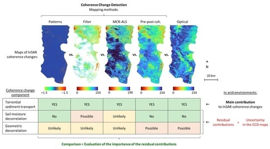
• Patterns. The CCD method based on the coherence between consecutive SAR images. Changes in the average spatial distribution of the coherence (Figure 2a).

Since the soil moisture decorrelation only affects the coherence during and shortly after rain- and snowfall events, the idea is to avoid these temporal effects and compare the spatial distribution—or pattern—of the InSAR coherence before the event and after the temporal effects of the changes in soil moisture. However, there is still geometric decorrelation. Since its magnitude is aleatory in time, the idea is to minimise it by approximating the spatial patterns of the coherence before and after the event to the average coherence between consecutive SAR images not disturbed by the soil moisture decorrelation. Thus, the CCD map is calculated as

$${chg}_{patterns}\left(x,y,v\right)=\frac{{av}_{v,2}-{av}_{v,1}}{av\left({av}_{v,1}+{av}_{v,2}\right)}$$

(2)

where $x$, $y$ are the spatial coordinates; $v$ identifies the torrential sediment transport event; subscripts $1$ and $2$ identify, respectively, the periods before and after the soil moisture changes caused by the rain- or snowfall event linked to the sediment transport; $av$ stands for average; and ${av}_{v,1}$ and ${av}_{v,2}$ are the undisturbed spatial patterns of InSAR coherence before and after the torrential sediment transport event:

$${av}_{v,u}=\frac{\sum _{j=i_{v,u}}^{f_{v,u}}\left(coh\left(x,y\right)\right)}{\left(f_{v,u}-i_{v,u}\right)+1},v,i_{v,u},f_{v,u}\in \mathbb{N},u\in \left\{\mathrm{1,2}\right\}$$

(3)

where $u$ is either 1 or 2 and identifies, respectively, the periods before and after the soil moisture decorrelation caused by the rain- or snowfall event linked to the sediment transport; $coh$ stands for the InSAR coherence between consecutive SAR images; and $i_{v,u}$ and $f_{v,u}$ identify, respectively, the first and last raster or map of InSAR coherence of the pattern, numbered in chronological order.

• Filter. The CCD method based on the coherence between consecutive SAR images. Selection of the “abnormal” values of the InSAR coherence time series (Figure 2b).

The idea is similar to the patterns method: if the torrential sediment transport events stand out because of the loss of coherence that they cause, the idea is to map only the abnormal values of coherence. In other words, this method looks for changes in the InSAR coherence in the temporal dimension of the data instead of the spatial dimension: the abnormal values are the outliers of the time series of InSAR coherence, defined as the values lower than a standard deviation below the median of the time series of the given point or pixel. So the CCD map is built as the map of coherence after applying the following filter:

$${chg}_{filter}\left(x,y,r\right)=\left\{\begin{array}{c}\varnothing ifcoh\left(x,y,r\right)\ge med\left(x,y\right)-std.dev\left(x,y\right)\\ coh\left(x,y,r\right)ifcoh\left(x,y,r\right)<med\left(x,y\right)-std.dev\left(x,y\right)\end{array}\right.$$

(4)

where $r$ identifies the raster or map of coherence between consecutive SAR images, i.e., the time; $med$ stands for median; and $std.dev$ stands for standard deviation. Again, since the geometric decorrelation is aleatory in time and always presents a similar distribution in space, and the soil moisture decorrelation also has an approximately constant distribution in space, none of these effects should affect the maps obtained with the filter method, and only the soil moisture decorrelation could have a minor role in when a change is detected, but not where.

• MCR-ALS. The CCD method based on the coherence between consecutive SAR images. Mixture resolution technique to identify the spatial distribution of permanent InSAR coherence changes within a set of SAR images (Figure 2c).

This is an algorithm that identifies patterns within a dataset—as many patterns as previously determined. Thus, the idea is that if the imposed number of patterns—called components in MCR-ALS—is high enough and the torrential sediment transport events significantly alter the InSAR coherence, then the variations in InSAR coherence caused by these events should be “captured” by individual components. The idea is better contextualised in the explanation of the MCR-ALS that can be found later in this section, but the result should be that MCR-ALS eliminates the “noise” that is not uniquely related to a particular event, i.e., the geometric and soil moisture decorrelations—which should present a similar spatial distribution from one event to another.

• Pre–post coherence. The CCD method based on the coherence between non-consecutive SAR images. Coherence between SAR images straddling an event (and its temporal effects) (Figure 2d).

This method was probably the first attempt to build CCD maps, and the idea is similar to that of the patterns method, although more direct: the soil moisture decorrelation is avoided by computing the coherence between the last SAR image before the rain- or snowfall event triggering the torrential sediment transport and the first SAR image after the temporal soil moisture decorrelation caused by the event. Thus, apart from torrential sediment transport, the only factor affecting the InSAR coherence that may remain is the geometric decorrelation, whose relevance can be evaluated with the perpendicular baseline: if the perpendicular baseline is large (tens or hundreds of metres), then the geometric decorrelation might be relevant in rugged-relief areas; if it is small (few metres), then the geometric decorrelation will probably be insignificant.

Figure 2. Explanatory diagram of the CCD mapping methods.

Figure 2. Explanatory diagram of the CCD mapping methods.

In addition, in the optical method, added as a non-CCD method in the evaluation of the CCD results, some post-processing is applied to enhance the detection of changes in the observed surface, which consists of (i) working only with the red band of the RGB images, since we verified that, because of the chromatic context, it is more sensitive to changes; (ii) normalising each image with its average value (of the red band) in the study area; and (iii) computing the difference between an image before and an image after each rain- or snowfall event triggering torrential sediment transport:

$${chg}_{optical}\left(x,y,v\right)=\left\{\begin{array}{c}\left|R_2\left(x,y,v\right)·\frac{av\left(R_1\right)}{av\left(R_2\right)}-R_1\left(x,y,v\right)\right|ifav\left(R_1\right)\ge av\left(R_2\right)\\ \left|R_2\left(x,y,v\right)-R_1\left(x,y,v\right)·\frac{av\left(R_2\right)}{av\left(R_1\right)}\right|ifav\left(R_1\right)<av\left(R_2\right)\end{array}\right.$$

(5)

where $R_1$ and $R_2$ are the red bands of the images before and after the event, respectively.

Note that the proposed methods cover a range of different degrees of complexity and sensitivity to the geometric and soil moisture decorrelations (

Table 1. Characteristics of the proposed mapping methods.

Method	Technique	SAR Images	Soil Moisture Decorrelation	Geometric Decorrelation
Patterns	CCD	Consecutive	No	Unlikely
Filter	CCD	Consecutive	Possible	Unlikely
MCR-ALS	CCD	Consecutive	Unlikely	Unlikely
Pre–post coherence	CCD	Non-consecutive	No	Possible
Optical	Optical	-	No	Possible

), in such a way that the comparison of their results will allow us to evaluate the importance of each decorrelation and, thus, the degree of uncertainty that they introduce into the CCD maps.

The results obtained with the different CCD mapping methods are compared both qualitatively and quantitatively. Qualitatively, we analyse if the methods detect sediment transport (erosion or sedimentation) in the same areas. Quantitatively, we measure numerically how similar the maps obtained with the different methods are, using the Intersection over Union (IoU) ratio, which compares the methods in pairs. For such a comparison, this ratio requires a binary conversion of the maps into changes (torrential sediment transport) and non-changes, since it is defined as the ratio between the area where both methods detect changes (intersection) and the area where one or both methods detect changes (union). The procedure is described in the next section.

Finally, as MCR-ALS stands out among the mapping methods for being a technique that is possibly never used in geomorphology, a more complete explanation of this method concludes this section. MCR-ALS is an algorithm developed in chemometrics to resolve complex chemical mixtures. Multivariate Curve Resolution (MCR) is a family of algorithms that address the mixture analysis problem by expressing the original data (the mixture) as a bilinear combination of pure species [33]. In particular, MCR-ALS solves the MCR bilinear model using a constrained Alternating Least Squares (ALS) algorithm. The main advantages of MCR-ALS are that no previous knowledge about the pure species is needed, but, at the same time, if such knowledge is available, it can be introduced in the model through the constraints. This makes MCR-ALS a highly flexible and versatile technique suitable to be applied to a great variety of fields and data [34], such as geomorphology.

From the mathematical point of view, the MCR-ALS model can be expressed in the following matrix form [35]:

$$D=C·S^T+E$$

(6)

where $D$ is the input mixture data, $C$ is the concentrations, and $S$ the spectra of the pure species or, in terms of this study, $D$ contains the rasters or maps of coherence between consecutive SAR images (one raster at each column), $C$ contains the spatial distributions of the components (one component at each column), and $S$ contains the weights of the bilinear combinations. The superscript ${}^T$ stands for the transposed matrix, and the matrix $E$ contains the residuals not explained by the pure species or components of matrix $C$. Thus, the input data are the mixture (the rasters of InSAR coherence) and the number of components, and the outputs are the concentrations of the pure species (the spatial distributions of the components) and their spectra (the weights of each component in each raster). The dimensions of the matrices are $D$ ($p$ × $r$), $C$ ($p$ × $c$), $S$ ($r$ × $c$), and $E$ ($p$ × $r$), where $p$ is the number of pixels of the rasters of InSAR coherence, $r$ is the number of rasters, and $c$ is the number of components. Note that the construction of the matrix $D$ requires a geometrical conversion of each raster of coherence from an ($i$ × $j$) matrix to an ($i·j$ × 1) vector (where $i·j$ = $p$), a conversion that will have to be reverted (from ($i·j$ × 1) vectors to ($i$ × $j$) matrices) to obtain the spatial distributions of the components. In other words, the rasters can be understood as matrices of $i$ rows and $j$ columns ($i$ and $j$ multiplied by the spatial resolution of the rasters give the geographical dimension of the rasters), and their pixels—the cells of the matrices—need to be reordered into a single column in the construction of matrix $D$.

The MCR-ALS is an iterative method that begins with an initial estimation of either $C$ or $S$, usually obtained using methods based on evolving factor analysis (EFA) or SIMPLISMA (Simple-to-Use Interactive Self-Modelling Mixture Analysis) [34]. Then, matrices $C$ and $S$ are optimised by iteratively solving Equation (6) with ALS. During the ALS optimisation, several constraints can be applied to $C$ and $S$, such as non-negativity, selectivity (some values are forced to zero), unimodality, or closure (a certain sum is forced to a constant value; for instance, mass conservation) [34,35]. Convergence is achieved (i) when a certain percentage of explained variance is reached, (ii) when the lack of fit is under a given threshold, (iii) when the matrices $C$ and $S$ do not evolve anymore (which is usually measured with the standard deviation of the residuals between the experimental—input—and the ALS-calculated matrices of consecutive iterations), or (iv) when a maximal preselected number of iterations is reached [34,35]. The main drawback of MCR-ALS is that it may fail to converge to the optimal $C$ and $S$ matrices [35]. Thus, in order to verify that the correct solution has been achieved, it is essential to check and compare the lack of fit ($LoF$, Equation (7)) of the solutions obtained with ALS and principal component analysis (PCA) and check the percentage of explained variance ($R^2$, Equation (8)) [35,36]:

$$LoF\left(\%\right)=100·\left(\sqrt{\frac{\sum _{k,l}\left({e_{k,l}}^2\right)}{\sum _{k,l}\left({d_{k,l}}^2\right)}}\right)$$

(7)

$$R^2\left(\%\right)=100·\left(1-\frac{\sum _{k,l}\left({e_{k,l}}^2\right)}{\sum _{k,l}\left({d_{k,l}}^2\right)}\right)$$

(8)

where $e_{k,l}$ are the elements of the matrix $E$ and $d_{k,l}$ are the elements of the matrix $D$. The optimal number of components can be found by comparing the performance of MCR-ALS models using a different number of components [36]. Its initial estimation is often obtained with PCA [33]. Further details about the MCR-ALS can be found in the literature [33,34,35,36].

2.4. Procedure

The mapping of the area affected by a torrential sediment transport event using CCD requires us to first (i) define the study area, (ii) download the SAR images of the study period (Table A1), (iii) calculate the rasters of InSAR coherence (Equation (1)), and (iv) identify the events that occurred during the study period, i.e., the dates when such events happened and the duration of the temporal soil moisture decorrelation. These steps were already carried out in a previous work [27], and the results are used here as a starting point, i.e., input data (Figure 3a). Then, with the rasters of coherence, the dates of the events, and the duration of the temporal effects related to each event, i.e., the soil moisture decorrelation, the procedure is different for each method (Figure 3):

• Patterns:

  1.

  Calculation of the average maps of coherence between consecutive SAR images before the event and after its temporal soil moisture decorrelation (Equation (3)).

  2.

  Mapping of the events (Equation (2)).

• Filter:

  1.

  Application the filter (Equation (4)).

  2.

  Mapping of the events, i.e., generation of the maps for the relevant dates.

• MCR-ALS:
  • Determination of the number of components of the MCR-ALS model. As a first guess, we consider one component (or one spatial pattern or distribution of InSAR coherence) between the events and two components during an event (temporal and permanent changes in the InSAR coherence).
  • Application of the MCR-ALS algorithm. In this study, the initial estimation of the matrix C was obtained using a modified SIMPLISMA algorithm; a non-negativity constraint was applied to both matrices S and C, using, respectively, the fast non-negative least squares and the forced-to-zero methods [34]; the convergence was achieved when the standard deviation of the residuals between the elements of the experimental and the ALS-calculated matrix D changed less than 0.01% between two consecutive iterations.
  • Verification of the weights of the components at each raster of coherence between consecutive SAR images to validate the number of components determined in step 1. Ideally, for each event, there should be at least one component that is only relevant in the rasters related to that event and other components with a random weight along the series of rasters (i.e., over time). The former will represent the changes in the surface related to the event, whereas the latter represents and eliminates the other components of the decorrelation.
  • If needed, iteration of steps 1 to 3.
• Pre–post coherence:
  • Mapping the events, i.e., computation of the coherence between the last SAR image before the rain- or snowfall event triggering the torrential sediment transport, and the first SAR image after the temporal soil moisture decorrelation caused by the event.
• Optical:
  • Downloading of the images for the relevant dates (Table A2).
  • Normalisation of the red band of the images by their average (Equation (5)).
  • Mapping of the events (Equation (5)).

Note that the methods based on the coherence between consecutive SAR images (namely, patterns, filter, and MCR-ALS) are applied to the whole series of rasters, including events and “non-events”. Nevertheless, the previous analysis to identify the occurrence of the events and the duration of the temporal disturbances in the InSAR coherence is necessary as it provides the required input information. The pre–post coherence and the optical methods greatly benefit from such an analysis since it allows us to only work with the relevant dates.

Finally, regarding the quantitative comparison of the results obtained with each CCD mapping method, i.e., the IoU ratio, the procedure used is as follows (Figure 3c):

• Uniformisation of the resolution of the maps of all the methods.
• Binary conversion of the maps obtained with each method into changes (hypothetically, erosion or sedimentation) and non-changes:

$${\xi }_m\left(x,y,v\right)=\left\{\begin{array}{c}0ifcoh\left(x,y,v\right)\ge {thres}_m\\ 1ifcoh\left(x,y,v\right)<{thres}_m\end{array}\right.$$

(9)

where ${\xi }_m$ is the binary value after the conversion for the mapping method $m$, and ${thres}_m$ is the threshold of the method $m$ used for the conversion. Since the sensitivity of each method to the surface changes is different, the criterion to determine the threshold is that the extension of the area where changes are detected—or, in other words, the number of pixels where the coherence is lower than the threshold—is the same for all four CCD mapping methods. As a basis for comparison, a threshold value of 100 was applied to the pre–post coherence method (for an InSAR coherence normalised to the range from 0 to 254), but the results should remain essentially the same if a different reference was used.

3.

Sum of the binary maps. Only three values are possible in the resulting map: 0 where either of the two methods being compared detects any change; 1 where only one of the two methods detects changes; and 2 where both methods detect changes, i.e., the intersection.

4.

IoU ratio:

$$IoU\left(m_1,m_2,v\right)=\frac{A_2}{A_1+A_2}$$

(10)

where $m_1$ and $m_2$ are the two mapping methods being compared, and $A_1$ and $A_2$ are the area or, equivalently, the number of pixels ($p$) of the map obtained in step 3 (the sum of the binary maps) that have a value of 1 and 2, respectively. The IoU ratio, as defined in Equation (10), can take values in the range of [0, 1].

The IoU ratio may be very sensitive to slight discrepancies between the maps of the methods being compared. For instance, two methods could detect surface changes along the same section of a gully, which should correspond to a maximal IoU ratio, but a small difference in the width of the stripe where the changes are detected, caused by a different sensitivity of the methods, may decrease the IoU ratio to a very low value. Therefore, in order to reduce such over-sensitivity, we base the quantitative comparison on the IoU ratio over a 3 × 3-pixel window, which is also calculated using Equation (10) but after applying a tolerance filter of ±1 pixel on the map obtained in step 3 (the sum of the binary maps). At a given pixel $p$, this filter is defined as follows:

• If the map obtained in step 3 has a value of 0 at the pixel $p$, then the value of the filtered map remains 0 at the pixel $p$.
• If the map obtained in step 3 has a value of 2, then the value remains 2.
• If the map obtained in step 3 has a value of 1, then:
  • If the map obtained in step 3 has a value of 2 somewhere in a 3 × 3-pixel window centred at the pixel $p$, then the filtered map takes a value of 2 at the pixel $p$.
  • Otherwise, the value of the filtered map remains 1 at the pixel $p$.

In the case of the filter method, the IoU ratios are calculated only in the pixels selected according to Equation (4), i.e., in the pixels where the filter method provides data.

The idea behind this tolerance filter is that, if two methods indicate the same spatial distribution of surface changes and their only difference is the extent, the numerical comparison should not penalise this discrepancy as much as if their spatial distributions were completely different or the changes were detected at different locations.

3. Results

The results obtained with the four CCD mapping methods show a general agreement at the scale of the study area: the areas affected by torrential sediment transport are (i) wide areas along the main channels of the proximal fans, especially in the northern ones; (ii) the slopes of the northern summits above 3500 m.a.s.l.; (iii) high-altitude torrential materials located at 3900–4000 m.a.s.l. in the southeast of the study area; and (iv) other more localised and less extensive torrential materials in the southern outcrops (Figure 4 and Figure 5). When observing the results, note that the patterns method (leftmost column in Figure 4 and Figure 5) provides extra information in comparison to the other methods: positive values in the results indicate an increase in the stability of the radar signal after an event, whereas negative values indicate the opposite. Thus, changes are represented by large values (either positive (blue) or negative (orange to red)), which, in the case of agreement, should be located in the areas with low values (red) for the other methods. Regarding the MCR-ALS model, after a few iterations, the number of components was fixed at 30 components, achieving a lack of fit of 4.195% and 1.493% for the ALS and PCA, respectively, and 99.824% of explained variance.

Logically, the degree of coincidence between the CCD mapping methods at the scale of a gully or an alluvial fan diminishes, as can be observed with the IoU ratio (Figure 6). Numerically, the average IoU ratio for the five events that occurred during the study period (April 2015–June 2018), with a tolerance of ±1 pixel, as described in Section 2.4, ranges from 42 to 61%, depending on the pair of methods being compared (

Table 2. Average Intersection over Union (IoU) ratios between the CCD mapping methods for the five events that occurred during the study period, with a tolerance of ±1 pixel (without brackets) and ±2 pixels (in brackets).

	Pre–Post Coh.	Patterns	Filter	MCR-ALS
Pre–post coh.	100%	45% (57%)	61% (71%)	61% (69%)
Patterns		100%	44% (58%)	42% (64%)
Filter			100%	56% (66%)
MCR-ALS				100%

). If the tolerance is increased to ±2 pixels, the IoU ranges from 54 to 71% (Table 2). This increase shows the high sensitivity of the IoU to small discrepancies between the maps being compared.

An initial analysis of the results obtained with each method shows the following.

• The patterns method is less sensitive to changes in the observed surface because it compares averages. For the same reason, this method is not able to distinguish between rain- or snowfall events that occurred very close together. On the other hand, it appears to be the only method not affected by snow cover (see event 4, top row in Figure 5), and the sign of its results provides extra information in comparison to the other methods. This point will be further discussed in the next section.
• The filter works well and provides useful results that are consistent with the other methods, but since it does not provide information everywhere for every event, its maps are not as clear as for the other methods.
• The MCR-ALS provides results very similar to the pre–post coherence but at a higher cost, if the dates of the events and the duration of the associated temporal soil moisture decorrelation were known a priori. However, if this information is not known a priori, the cost-benefit in comparison to the pre-post coherence method is debatable. Another advantage of the MCR-ALS is that it is able to distinguish between events that occurred close together. Finally, MCR-ALS appears to be sensitive to aeolian sediment transport, which, based on the meteorological records, could explain its discrepancy with the other methods in event 2 (middle row in Figure 3). According to the available data, this is the only event among the five that occurred during the study period in which significant aeolian sediment transport occurred.
• The pre–post coherence offers much clearer results than the filter at a lower cost, provided that the dates of the events and the duration of the associated temporal soil moisture decorrelation were already known. However, similar to the patterns method, it is not able to distinguish between rain- or snowfall events that occurred very close together.
• Finally, the optical images appear to be of very limited help. On the one hand, this is because of the obstruction caused by cloud cover (either the direct obstruction or their projected shadow) and, in event 4, the chromatic distortion of the snow cover. And on the other hand, this is because even without those limitations, the optical method is less sensitive than the CCD methods (see event 3 in Figure 4). Nevertheless, the analysis of the optical results at a more local scale (a gully or an alluvial fan) shows changes in the same areas as the CCD-based maps (see, for instance, the comparison with a field campaign in the next section).

4. Discussion

4.1. Analysis of the Mapping Methods

According to the reasoning discussed in Section 2.3 (Table 1), the only CCD mapping method exposed to decorrelation not caused by changes in the observed surface is the pre–post coherence (it may be affected by the geometric decorrelation). However, no correspondence is observed between how much the topographic relief is visible in the maps (fourth column in Figure 4 and Figure 5) and the perpendicular baseline (Table A2). In fact, according to the IoU ratios, the pre–post coherence is the method with the largest coincidence with the other ones (Table 2). Furthermore, for all of the four CCD mapping methods, the changes detected in the surface are neither always detected in the same areas, nor are they detected with the same intensity (Figure 4 and Figure 5). In other words, the spatial distribution of the detected changes varies from one event to another. If these changes were due to geometric decorrelation, not only should the intensity of the changes correlate with the perpendicular baseline, but their spatial distribution should also be similar for all the events, which is not the case.

Regarding the eventual soil moisture decorrelation, the two CCD methods that might be sensitive to it, namely the filter and the MCR-ALS (Table 1), never indicate changes in areas where the other methods do not detect changes too, especially the pre–post coherence method (second, third, and fourth columns in Figure 4 and Figure 5).

Consequently, we conclude that, in the area and period of study, neither the geometric nor the soil moisture decorrelation that may remain in the CCD maps are significant. Thus, the areas marked on the CCD maps have probably experienced erosion or sedimentation related to flash floods, even if these areas happen to be some of the zones that are the most susceptible to the geometric (the gullies) and/or the soil moisture decorrelation (e.g., the alluvial fans).

Nevertheless, in the patterns method (first column in Figure 4 and Figure 5), in some areas and for some events, parallel patterns with opposite signs are observed on the maps. See, for instance, the northern gullies in event 2 or the mid-latitude volcanic cone in events 2 and 3 (Figure 5). Although the meaning of the sign of the results is not clear yet, we wonder if such features could be the signature of the effects of the perpendicular baseline. In such a case, the patterns method could be a technique to detect such effects in an easier and more economical way than, for instance, processing different SAR datasets obtained with different geometries. This point remains to be better analysed in further research.

In any case, the comparison with other sources of data, specifically the optical Sentinel-2 images and field observations, is also satisfactory. The validation with the optical images is very limited due to the cloud cover and the snow, but in the local areas where the comparison with the CCD results is possible, the optical results show changes in the same areas as the most significant changes detected using the CCD methods. However, the optical images seem to be insensitive to the smaller changes observed in the CCD-based maps. In other words, the CCD methods are more sensitive to changes in the observed surface than the comparison between optical images—as already stated in the Introduction. Regarding the field observations, the comparison of the results of the CCD methods with a field campaign that mapped the sediments mobilised by event 5 (last row in Figure 5) shows very good agreement (Figure 7).

Figure 7. Comparison of the results for event 5 with a field campaign. See the location of the mapped area in Figure 5. For ease of comparison, the left and right columns show the same maps with and without the field campaign on top, respectively.

Figure 7. Comparison of the results for event 5 with a field campaign. See the location of the mapped area in Figure 5. For ease of comparison, the left and right columns show the same maps with and without the field campaign on top, respectively.

Thus, the next step in the mapping of torrential sediment transport based on CCD would be to build probability maps showing the areas where such phenomena are most likely to occur. Such maps would require a statistical analysis of historical records that, unfortunately, do not exist, especially in such remote areas. However, SAR data do offer a historical archive that could be analysed retrospectively. This could also be a task for further research. In the meantime, the data analysed in this study already allow us to perform an approximation of a 3-year return period probability map (Figure 8), since the study period spans over approximately three years: the average of the binary change maps of the five events (see Section 2.4). Given the scarcity of information in a region like the study area, this information is already highly valuable.

4.2. Comparison with the Literature

Since this is not the only study on the use of CCD to map torrential sediment transport events in arid environments, it is worth making a brief comparison with the methods, results, and observations of other studies in the literature.

Thus, regarding the applied methods, it is interesting to note that PCA, which is a method close to MCR-ALS, has also been used in CCD aiming to eliminate the components of the decorrelation not related to changes in the observed surface [24]. Logically, the most direct method, which is to calculate the coherence between an image before a rain- or snowfall event and an image after the temporal effects on the InSAR coherence caused by the event—i.e., the soil moisture decorrelation—has also been applied in previous studies [16]. The pattern method follows the same idea. However, the advantage in our case is that, in our previous study [27], we determined the period affected by the temporal changes in coherence based on the direct analysis of the InSAR coherence data instead of using a model (for instance, of the decorrelation related to humidity changes), and working only with the coherence between consecutive SAR images, rather than with the coherence rasters between all possible pairs of SAR images. Thus, we believe that our methodology is much more efficient and more precise in determining the duration of the temporal effects. As a final observation related to the methodology, the amount of precipitation was found to affect the duration of temporal changes in coherence, but not their magnitude [16]. We agree, but our previous study [27] suggests that we should be careful since it might also be due to a lack of representativeness of the meteorological data, which would prevent observing a correlation between the amount of precipitation and the magnitude of the temporal loss of coherence. In any case, the results of the methods that might be affected by the temporal soil moisture decorrelation—namely, the filter and, perhaps, the MCR-ALS to a lesser extent—and the results of the methods not affected by these effects coincide, which supports the mentioned hypothesis.

Moving on to the analysis of the results, in the literature, changes in InSAR coherence are detected in the same areas, from the upper reaches of the gullies to the alluvial fans [4], but with nuances between studies. Some observe a decrease in the decorrelation downstream caused by a progressive reduction in the flow of water and sediments due to evaporation and infiltration [1]. In our case, we do detect a less important decorrelation in the middle reaches, but it increases again in the lower reaches until the alluvial fan. Precisely in the alluvial fans, several studies (e.g., [26]) conclude that their whole surface is affected by sediment transport (in principle, sedimentation). However, we do not always detect changes in all the alluvial fans, nor in their entire extent. In fact, for example, the field campaign included in the discussion shows precisely an example in which the sediment transport was mainly limited to the main channels of the alluvial fan. Another interesting aspect is that, although other studies have also detected changes in coherence along the gullies [1,4,16], quite often, it is not confirmed whether the changes are related to real changes in the surface or to geometric effects related to the perpendicular baseline. In a similar way, apart from the gullies, the literature also notes decorrelation in areas of steep relief [15], which are often also associated with geometric decorrelation. In our case, the comparison between different mapping methods allows us to conclude that, indeed, there has most likely been sediment transport in these areas. Moreover, this comparison between methods that have different sensitivities to the effects of the perpendicular baseline and soil moisture changes has allowed us to relate the correlation that we observe between loss of coherence and surface geology and topographic relief (alluvial fans and gullies), which has also been observed by other authors [24], to real changes in the surface, despite the correlation that also exists between the geometric and the soil moisture decorrelations and surface geology and topographic relief. The fact is that, on the one hand, the areas that are the most susceptible to decorrelation due to torrential sediment transport are the areas of mobilisation and the deposition of sediments, i.e., the upper reaches of the gullies and the alluvial fans, respectively; but, on the other hand, these are also the areas that are the most susceptible to the geometric and soil moisture decorrelations: gullies are areas of very rugged topographic relief and, therefore, the areas where errors due to the perpendicular baseline are maximal, and the alluvial fans are the most porous areas, able to retain moisture for a longer time, so these are the areas where the errors due to soil moisture changes are maximal too. As a last remark to close this discussion, as already stated in the literature [4,11,18], our results show that the CCD methods are more sensitive to changes in the observed surface than optical images, which positions CCD as a highly useful technique despite the uncertainties that remain to be resolved.

5. Conclusions

This paper analysed the uncertainties related to the decorrelation caused by the perpendicular baseline and changes in soil moisture on the maps of torrential sediment transport in arid environments based on InSAR coherence-change detection (CCD). To this end, the results of four CCD mapping methods, each one with a different sensitivity to each component of the decorrelation, were compared between each other and with two mapping methods of a different nature: changes in satellite optical images and a field campaign.

Both the comparison between CCD methods and the comparison of the CCD methods with the optical method and the field observations lead to the conclusion that CCD maps are reliable in the identification of the zones affected by sediment transport, although the precision in the delimitation of the affected area remains an open issue. However, highly rugged relief areas still require a thorough analysis of the results in order to discard errors related to the perpendicular baseline.

Based on the discussion of the results, a combination of the pre–post coherence and the patterns methods would be the most convenient to map torrential sediment transport in an arid environment: the pre–post coherence method because it offers good results at a low cost, and the patterns method to check if there is any area where the geometric decorrelation (related to the perpendicular baseline) could be relevant. As a reminder, we mention that the pre–post coherence method computes the coherence between the last SAR image before the rain- or snowfall event triggering the torrential sediment transport, and the first SAR image after the temporal soil moisture decorrelation caused by the event, and the patterns method calculates the difference between the average coherence between consecutive SAR images during the period prior to the event not affected by soil moisture decorrelation from previous events, and the average coherence after the temporal soil moisture decorrelation caused by the event being analysed. Furthermore, the pre–post coherence requires the previous determination of the date of the event and the duration of the temporal effects.

Regarding future lines of research, several issues remain unresolved. First, the meaning of the sign of the patterns method’s results remains to be understood, as does whether parallel patterns on the maps of opposite signs are indeed related to topographic errors or not. Second, the probability map for torrential sediment transport could be improved using the entire historical archive of SAR data. And third, it would be interesting to have more in situ records of rainfall around the study area in order to compare the geographical distribution of the intensity of the torrential sediment transport detected by the CCD maps with the geographical distribution of the amount and intensity of precipitation.

References

1. Liu, J.G.; Black, A.; Lee, H.; Hanaizumi, H.; Moore, J.M. Land surface change detection in a desert area in Algeria using multi-temporal ERS SAR coherence images. Int. J. Remote Sens. 2001, 22, 2463–2477. [Google Scholar] [CrossRef]
2. Cohen, H.; Laronne, J.B. High rates of sediment transport by flashfloods in the Southern Judean Desert, Israel. Hydrol. Process. 2005, 19, 1687–1702. [Google Scholar] [CrossRef]
3. Aguilar, G.; Cabre, A.; Fredes, V.; Villela, B. Erosion after an extreme storm event in an arid fluvial system of the southern Atacama Desert: An assessment of the magnitude, return time, and conditioning factors of erosion and debris flow generation. Nat. Hazards Earth Syst. Sci. 2020, 20, 1247–1265. [Google Scholar] [CrossRef]
4. Cabré, A.; Remy, D.; Aguilar, G.; Carretier, S.; Riquelme, R. Mapping rainstorm erosion associated with an individual storm from InSAR coherence loss validated by field evidence for the Atacama Desert. Earth Surf. Process. Landf. 2020, 45, 2091–2106. [Google Scholar] [CrossRef]
5. Valdivielso, S.; Vazquez-Sune, E.; Custodio, E. Origin and variability of oxygen and hydrogen isotopic composition of precipitation in the Central Andes: A review. J. Hydrol. 2020, 587, 19. [Google Scholar] [CrossRef]
6. Reid, I.; Laronne, J.B.; Powell, D.M. Flash-flood and bedload dynamics of desert gravel-bed streams. Hydrol. Process. 1998, 12, 543–557. [Google Scholar] [CrossRef]
7. Moldenhauer-Roth, A.; Piton, G.; Schwindt, S.; Jafarnejad, M.; Schleiss, A.J. Design of sediment detention basins: Scaled model experiments and application. Int. J. Sediment Res. 2021, 36, 136–150. [Google Scholar] [CrossRef]
8. Malmon, D.V.; Reneau, S.L.; Dunne, T. Sediment sorting and transport by flash floods. J. Geophys. Res.-Earth Surf. 2004, 109, 13. [Google Scholar] [CrossRef]
9. Manzoni, M.; Molinari, M.E.; Monti-Guarnieri, A. Multitemporal InSAR Coherence Analysis and Methods for Sand Mitigation. Remote Sens. 2021, 13, 1362. [Google Scholar] [CrossRef]
10. Havivi, S.; Amir, D.; Schvartzman, I.; August, Y.; Maman, S.; Rotman, S.R.; Blumberg, D.G. Mapping dune dynamics by InSAR coherence. Earth Surf. Process. Landf. 2018, 43, 1229–1240. [Google Scholar] [CrossRef]
11. Song, Y.B.; Chen, C.B.; Xu, W.Q.; Zheng, H.W.; Bao, A.M.; Lei, J.Q.; Luo, G.P.; Chen, X.; Zhang, R.; Tan, Z.B. Mapping the temporal and spatial changes in crescent dunes using an interferometric synthetic aperture radar temporal decorrelation model. Aeolian Res. 2020, 46, 16. [Google Scholar] [CrossRef]
12. Gabriel, A.K.; Goldstein, R.M.; Zebker, H.A. Mapping Small Elevation Changes Over Large Areas: Differential Radar Interferometry. J. Geophys. Res. 1989, 94, 9183–9191. [Google Scholar] [CrossRef]
13. Bamler, R.; Hartl, P. Synthetic aperture radar interferometry. Inverse Probl. 1998, 14, R1–R54. [Google Scholar] [CrossRef]
14. Rosen, P.A.; Hensley, S.; Joughin, I.R.; Li, F.K.; Madsen, S.N.; Rodríguez, E.; Goldstein, R.M. Synthetic aperture radar interferometry—Invited paper. Proc. IEEE 2000, 88, 333–382. [Google Scholar] [CrossRef]
15. Schepanski, K.; Wright, T.J.; Knippertz, P. Evidence for flash floods over deserts from loss of coherence in InSAR imagery. J. Geophys. Res.-Atmos. 2012, 117, 10. [Google Scholar] [CrossRef]
16. Scott, C.P.; Lohman, R.B.; Jordan, T.E. InSAR constraints on soil moisture evolution after the March 2015 extreme precipitation event in Chile. Sci. Rep. 2017, 7, 9. [Google Scholar] [CrossRef]
17. Smith, L.C. Emerging applications of interferometric synthetic aperture radar (InSAR) in geomorphology and hydrology. Ann. Assoc. Am. Geogr. 2002, 92, 385–398. [Google Scholar] [CrossRef]
18. Ullmann, T.; Büdel, C.; Baumhauer, R.; Padashi, M. Sentinel-1 SAR Data Revealing Fluvial Morphodynamics in Damghan (Iran): Amplitude and Coherence Change Detection. Int. J. Earth Sci. Geophys. 2016, 2, 14. [Google Scholar] [CrossRef]
19. Jordan, T.E.; Lohman, R.B.; Tapia, L.; Pfeiffer, M.; Scott, C.P.; Amundso, R.; Godfrey, L.; Riquelme, R. Surface materials and landforms as controls on InSAR permanent and transient responses to precipitation events in a hyperarid desert, Chile. Remote Sens. Environ. 2020, 237, 18. [Google Scholar] [CrossRef]
20. Zebker, H.A.; Villasenor, J. Decorrelation in interferometric radar echoes. IEEE Trans. Geosci. Remote Sens. 1992, 30, 950–959. [Google Scholar] [CrossRef]
21. Lee, H.; Liu, J.G. Analysis of topographic decorrelation in SAR interferometry using ratio coherence imagery. IEEE Trans. Geosci. Remote Sens. 2001, 39, 223–232. [Google Scholar] [CrossRef]
22. Wegmüller, U.; Strozzi, T.; Farr, T.; Werner, C.L. Arid land surface characterization with repeat-pass SAR interferometry. IEEE Trans. Geosci. Remote Sens. 2000, 38, 776–781. [Google Scholar] [CrossRef]
23. Monti-Guarnieri, A.V.; Brovelli, M.A.; Manzoni, M.; D’Alessandro, M.M.; Molinari, M.E.; Oxoli, D. Coherent Change Detection for Multipass SAR. IEEE Trans. Geosci. Remote Sens. 2018, 56, 6811–6822. [Google Scholar] [CrossRef]
24. Kim, J.; Dorjsuren, M.; Choi, Y.; Purevjav, G. Reconstructed Aeolian Surface Erosion in Southern Mongolia by Multi-Temporal InSAR Phase Coherence Analyses. Front. Earth Sci. 2020, 8, 9. [Google Scholar] [CrossRef]
25. Gaber, A.; Abdelkareem, M.; Abdelsadek, I.S.; Koch, M.; El-Baz, F. Using InSAR Coherence for Investigating the Interplay of Fluvial and Aeolian Features in Arid Lands: Implications for Groundwater Potential in Egypt. Remote Sens. 2018, 10, 832. [Google Scholar] [CrossRef]
26. Ullmann, T.; Sauerbrey, J.; Hoffmeister, D.; May, S.M.; Baumhauer, R.; Bubenzer, O. Assessing Spatiotemporal Variations of Sentinel-1 InSAR Coherence at Different Time Scales over the Atacama Desert (Chile) between 2015 and 2018. Remote Sens. 2019, 11, 2960. [Google Scholar] [CrossRef]
27. Botey i Bassols, J.; Bedia, C.; Cuevas-González, M.; Valdivielso, S.; Crosetto, M.; Vázquez-Suñé, E. SAR Coherence in Detecting Fluvial Sediment Transport Events in Arid Environments. Remote Sens. 2023, 15, 3034. [Google Scholar] [CrossRef]
28. Valdivielso, S.; Vázquez-Suñé, E.; Herrera, C.; Custodio, E. Characterization of precipitation and recharge in the peripheral aquifer of the Salar de Atacama. Sci. Total Environ. 2022, 806, 14. [Google Scholar] [CrossRef]
29. Marazuela, M.Á.; Vázquez-Suñé, E.; Custodio, E.; Palma, T.; García-Gil, A.; Ayora, C. 3D mapping, hydrodynamics and modelling of the freshwater-brine mixing zone in salt flats similar to the Salar de Atacama (Chile). J. Hydrol. 2018, 561, 223–235. [Google Scholar] [CrossRef]
30. Valdivielso, S.; Hassanzadeh, A.; Vázquez-Suñé, E.; Custodio, E.; Criollo, R. Spatial distribution of meteorological factors controlling stable isotopes in precipitation in Northern Chile. J. Hydrol. 2022, 605, 12. [Google Scholar] [CrossRef]
31. Marazuela, M.A.; Vazquez-Sune, E.; Ayora, C.; Garcia-Gil, A.; Palma, T. The effect of brine pumping on the natural hydrodynamics of the Salar de Atacama: The damping capacity of salt flats. Sci. Total Environ. 2019, 654, 1118–1131. [Google Scholar] [CrossRef]
32. European Space Agency (ESA). Copernicus Open Access Hub. Available online: https://scihub.copernicus.eu/dhus/#/home (accessed on 25 June 2023).
33. De Juan, A.; Tauler, R. Multivariate Curve Resolution: 50 years addressing the mixture analysis problem-A review. Anal. Chim. Acta 2021, 1145, 59–78. [Google Scholar] [CrossRef]
34. Jaumot, J.; Gargallo, R.; de Juan, A.; Tauler, R. A graphical user-friendly interface for MCR-ALS: A new tool for multivariate curve resolution in MATLAB. Chemom. Intell. Lab. Syst. 2005, 76, 101–110. [Google Scholar] [CrossRef]
35. Tauler, R. Multivariate curve resolution applied to second order data. Chemom. Intell. Lab. Syst. 1995, 30, 133–146. [Google Scholar] [CrossRef]
36. Bedia, C.; Sierra, A.; Tauler, R. Application of chemometric methods to the analysis of multimodal chemical images of biological tissues. Anal. Bioanal. Chem. 2020, 412, 5179–5190. [Google Scholar] [CrossRef] [PubMed]
37. Dirección General de Aguas (DGA). Información Oficial Hidrometeorológica y de Calidad de Aguas en Línea; Ministerio de Obras Públicas, Gobierno de Chile: Santiago de Chile, Chile, 2023. [Google Scholar]
38. Gascoin, S.; Hagolle, O.; Huc, M.; Jarlan, L.; Dejoux, J.F.; Szczypta, C.; Marti, R.; Sánchez, R. A snow cover climatology for the Pyrenees from MODIS snow products. Hydrol. Earth Syst. Sci. 2015, 19, 2337–2351. [Google Scholar] [CrossRef]
39. Parajka, J.; Bloschl, G. Spatio-temporal combination of MODIS images—Potential for snow cover mapping. Water Resour. Res. 2008, 44, 13. [Google Scholar] [CrossRef]
40. Riggs, G.A.; Hall, D.K.; Román, M.O. MODIS Snow Products Collection 6 User Guide; National Aeronautics and Space Administration: Washington, DC, USA, 2016. Available online: https://modis-snow-ice.gsfc.nasa.gov/uploads/C6_MODIS_Snow_User_Guide.pdf (accessed on 29 March 2023).
41. Villaescusa-Nadal, J.L.; Vermote, E.; Franch, B.; Santamaria-Artigas, A.E.; Roger, J.C.; Skakun, S. MODIS-Based AVHRR Cloud and Snow Separation Algorithm. IEEE Trans. Geosci. Remote Sens. 2022, 60, 13. [Google Scholar] [CrossRef]
42. Parajka, J.; Bloschl, G. Validation of MODIS snow cover images over Austria. Hydrol. Earth Syst. Sci. 2006, 10, 679–689. [Google Scholar] [CrossRef]
43. Kilpys, J.; Pipiraite-Januskiene, S.; Rimkus, E. Snow climatology in Lithuania based on the cloud-free moderate resolution imaging spectroradiometer snow cover product. Int. J. Climatol. 2020, 40, 4690–4706. [Google Scholar] [CrossRef]
44. Hall, D.K.; Riggs, G.A. Accuracy assessment of the MODIS snow products. Hydrol. Process. 2007, 21, 1534–1547. [Google Scholar] [CrossRef]
45. Hüsler, F.; Jonas, T.; Riffler, M.; Musial, J.P.; Wunderle, S. A satellite-based snow cover climatology (1985-2011) for the European Alps derived from AVHRR data. Cryosphere 2014, 8, 73–90. [Google Scholar] [CrossRef]
46. Busetto, L.; Ranghetti, L. MODIStsp: An R package for automatic preprocessing of MODIS Land Products time series. Comput. Geosci. 2016, 97, 40–48. [Google Scholar] [CrossRef]
Figure 1. Study area: sub-basins of Talabre and Socaire (c) of the Salar de Atacama Basin (b), northern Chile (a). The surficial geology is shown in (d), together with the main hydrographic network; the topographic slope is shown in (e).
Remotesensing 15 04964 g001
Figure 3. Flow chart of the mapping procedures and the comparison of the results obtained with each method.
Remotesensing 15 04964 g003
Figure 4. Results (i): events 1 to 3. Comparison between the different mapping methods (columns) for each torrential sediment transport event that occurred during the study period (rows). The rightmost images are the pairs of optical images compared for each event, included in this figure to ease the interpretation of the changes mapped with them. The dates of the time periods covered by each map are indicated below, as well as the rainfall accumulated during that event at the meteorological station in the Salar de Atacama Basin that registered the largest amount, and the maximal daily decrease in the snow cover in the study area during the event (thaw). Note that, although the colour legend is not the same for every method, their meaning remains the same (except for the patterns method): red indicates changes, while blue indicates stability. For the patterns method, the brightest colours indicate changes, while the darkest (blue) colours indicate stability. There is a general agreement in the detection of the areas affected by torrential sediment transport between the CCD methods, except for the MCR-ALS map of event 2. According to the meteorological records, this may be due to aeolian sediment transport.
Remotesensing 15 04964 g004
Figure 5. Results (ii): events 4 and 5. See the caption of the previous figure for more information. The red rectangles in event 5 are the extension of Figure 7. The eastern red band in event 4 (top row) is snow, which, interestingly, does not distort the map of the patterns method (first column).
Remotesensing 15 04964 g005
Figure 6. Sum of the binary maps generated for the calculation of the Intersection over Union (IoU) ratios between the CCD mapping methods, with a tolerance filter of ±1 pixel (see Section 2.4). Each column contains the comparison between two methods, and each row contains the comparisons for one event. The IoU ratios are the ratios between the green area and the sum of the green and the red areas.
Remotesensing 15 04964 g006
Figure 8. Probability map of torrential sediment transport based on the five events that occurred during the study period (April 2015–June 2018), elaborated with the pre–post coherence method.
Remotesensing 15 04964 g008