Article

Spatiotemporal Analysis of Landscape Ecological Risk and Driving Factors: A Case Study in the Three Gorges Reservoir Area, China

1
Three-Gorges Reservoir Area (Chongqing) Forest Ecosystem Research Station, School of Soil and Water Conservation, Beijing Forestry University, Beijing 100083, China
2
School of Ecology and Environment, Southwest Forestry University, Kunming 650224, China
*
Author to whom correspondence should be addressed.
Remote Sens. 2023, 15(19), 4884; https://doi.org/10.3390/rs15194884
Submission received: 27 August 2023 / Revised: 21 September 2023 / Accepted: 3 October 2023 / Published: 9 October 2023
(This article belongs to the Topic Aquatic Environment Research for Sustainable Development)

Abstract

:
Landscape ecological risk is considered the basis for regional ecosystem management decisions. Thus, it is essential to understand the spatial and temporal evolutionary patterns and drivers of landscape ecological risk. However, existing studies lack exploration of the long-term time series and driving mechanisms of landscape ecological risk. Based on multi-type remote sensing data, this study assesses landscape pattern changes and ecological risk in the Three Gorges Reservoir Area from 1990 to 2020 and ranks the driving factors using a geographical detector. We then introduce the geographically weighted regression model to explore the local spatial contributions of driving factors. Our results show: (1) From 1990 to 2020, the agricultural land decreased, while forest and construction land expanded in the Three Gorges Reservoir Area. The overall landscape pattern shifted toward aggregation. (2) The landscape ecological risk exhibited a decreasing trend. The areas with relatively high landscape ecological risk were primarily concentrated in the main urban area in the western region of the Three Gorges Reservoir Area and along the Yangtze River, with apparent spatial aggregation. (3) Social and natural factors affected landscape ecological risk. The main driving factors were human interference, annual average temperature, population density, and annual precipitation; interactions occurred between the drivers. (4) The influence of driving factors on landscape ecological risk showed spatial heterogeneity. Spatially, the influence of social factors (human interference and population density) on landscape ecological risk was primarily positively correlated. Meanwhile, the natural factors’ (annual average temperature and annual precipitation) influence on landscape ecological risk varied widely in spatial distribution, and the driving mechanisms were more complex. This study provides a scientific basis and reference for landscape ecological risk management, land use policy formulation, and optimization of ecological security patterns.

1. Introduction

With the continuous increase in human activities and the frequent occurrence of extreme global climate issues [1,2], the landscape pattern has changed significantly [3,4], leading to a series of new ecological and environmental challenges, including the expansion of construction land and increased pollution risk [5]. These issues have intensified the conflict between urbanization development and environmental protection, seriously threatening human well-being and the sustainable development of human–Earth ecosystems [6,7,8,9]. Landscape ecological risk refers to the possible adverse consequences of the interaction between landscape patterns and ecological processes under the influence of natural or human factors [5,10], an essential subfield of ecological risk under the perspective of spatial patterns [11]. Hence, accurately identifying, assessing, and characterizing the spatiotemporal dynamics of landscape ecological risks and their drivers can direct the construction of regional ecological security patterns.
The risk assessment of landscape ecology is often based on remote sensing data and can be divided into two assessment methods based on risk sources and sinks and landscape patterns. Compared with the former, the latter, in part, breaks away from the inherent “risk source identification—receptor analysis—exposure and hazard assessment” mode of traditional ecosystem assessment and directly evaluates the risk of landscape ecology based on spatial patterns [12]. In particular, a quantitative method of landscape ecological risk has been proposed based on “loss and probability multiplication.” This method relies on the product of landscape disturbance and vulnerability to estimate potential ecological loss [13], which is then combined with risk probability to calculate the specific risk value of the area [14,15,16]. To date, many regional studies involving cities [17], mining areas [10], watersheds [3], habitats [18], and islands [19] have adopted this method. However, most have focused on the ecological risk associated with rapid urbanization, while few studies have explored the differences in long-term time series. Clarifying this issue may provide insights to decision-makers regarding the changing risk trends in different development contexts and provide a basis for risk management.
Decision-makers have long sought effective management strategies for ecological risks. Accordingly, in addition to exploring the spatiotemporal variability of landscape ecological risks, further work is needed to identify the main drivers and evaluate the spatial heterogeneity of driving mechanisms. This has important practical significance for decision-makers to develop risk mitigation strategies and effectively allocate resources. Currently, the methods for exploring landscape ecological risk drivers mainly include the Pearson correlation analysis [20], grey relational analysis [21], and boosted regression tree [22]. However, these methods may ignore the spatial heterogeneity of drivers’ contributions. Recently, a geographical detector has been employed to explore the relationship between landscape ecological risks and their drivers [4,23,24]. This method can better detect spatial heterogeneity between variables, determine the influencing factors, and explain their interactions [25]. However, the geographical detector lacks local spatial expression of correlations between variables. Hence, the geographically weighted regression (GWR) model, a local modeling method, has been applied to analyze spatial relationships in ecological processes [26]. Therefore, this study innovatively introduces the GWR model and its centroid transfer process to explore the interrelationships between the variables, thus providing additional spatial details regarding the contributions of driving factors while also delving deeper into the driving mechanisms of landscape ecological risk change. The proposed methodology will support decision-makers in achieving accurate ecological risk management in local areas [27,28].
Having begun construction in 1994, the Yangtze Three Gorges Project (TGP) is the largest hydropower project in the world, playing a significant role in flood control, power generation, shipping, and water resource utilization. However, its construction has facilitated the implementation of other major projects, including water storage and migration in the Three Gorges Reservoir Area (TGRA). This has led to the inundation of large amounts of land, dramatic climate fluctuations, and significantly altered intensity of human activities. Moreover, considerable disturbance to the landscape pattern has occurred, resulting in ecological and environmental issues within the TGRA [29,30,31]. Therefore, evaluating the landscape ecological risk in the TGRA and exploring the causes of the risk have become important scientific research issues. Unfortunately, few studies have explored the landscape ecological risk of the TGRA under a long-term time series [32,33]. Moreover, regarding quantitative analysis of drivers, many studies have focused on the ranking of drivers [3,19,34,35], while few have explored the driving mechanisms of landscape ecological risk. Therefore, to address the current dearth of data related to change regulations and driving mechanisms of landscape ecological risk, this paper proposes a framework based on multi-type remote sensing data, taking the TGRA as an example. The primary aims of the study are to (1) explore the spatiotemporal characteristics of landscape pattern changes from 1990 to 2020; (2) evaluate the landscape ecological risk generated by landscape pattern changes; (3) rank the driving factors of landscape ecological risk using the geographical detector; (4) analyze local spatial contributions of drivers and the driving mechanisms of landscape ecological risk using the GWR model. Collectively, this work extends the exploration of the GWR model in terms of driving mechanisms and proposes theoretical insights for the exploration of landscape ecological risk and drivers on a long-term time series to provide a reference for scientific planning of land use and preservation of ecological balance in the TGRA.

2. Materials and Methods
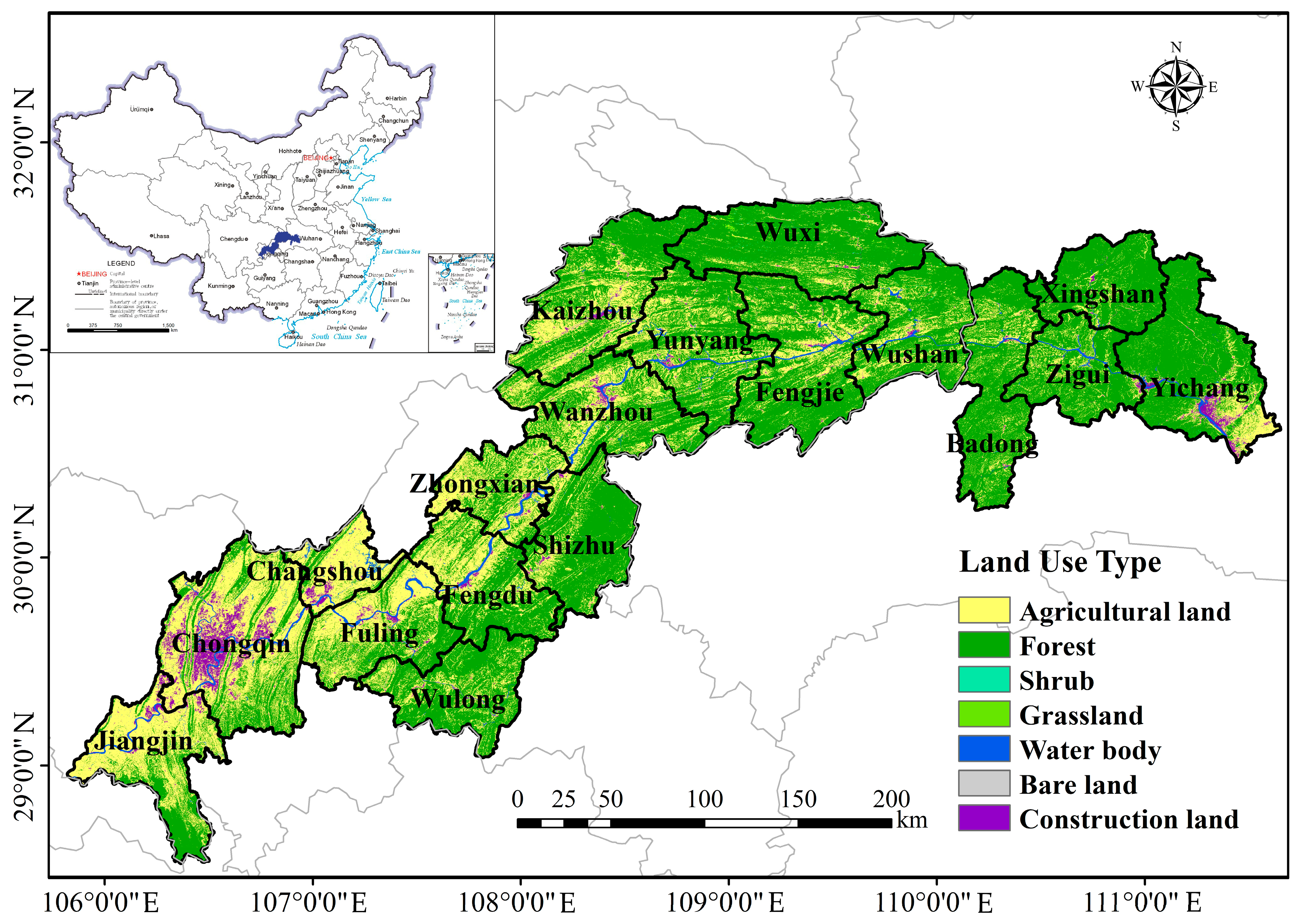
2.1. Study Area

The TGRA (106°20′–110°30′E, 29°00′–31°50′N) refers to the 26 districts in China inundated by the TGP (Figure 1), the construction of which began in 1994 and was completed in 2006, with an area of 5.8 × 10⁴ km2 [36]. The TGRA is located within the Sichuan basin and the middle reaches of the Yangtze River in China. It has high topography in the east and low topography in the west, with mountains and hills accounting for 74% and 22% of the total area, respectively, representing a typical mountainous area. The TGRA comprises primarily forests and agricultural land. Due to its topography, the TGRA has more sloping agricultural land that is vulnerable to water and soil loss. The TGRA belongs to the humid subtropical climate, with an average annual temperature of 10–14 °C in the mountainous area and 17–19 °C in the valley region. The average annual precipitation is 1000–1200 mm. Moreover, the TGRA has an uneven seasonal distribution, with the precipitation from April to October accounting for >80% of the annual precipitation. In addition, the peripheral mountains receive more precipitation than the river valleys. The resettlement of immigrants, infrastructure construction, and the restructuring of the agricultural and forestry industries resulting from the TGP construction caused dramatic changes in its population and economic structure [31]. In 2020, the GDP of the TGRA was 969.15 billion yuan, the population was 15.61 million, and the population density was 269 people/km2, far beyond the national average [36]. Due to specific climatic and geographical conditions as well as strong human interference, the region is affected by frequent earthquakes, collapses, landslides, mudslides, and other disasters that severely impact the ecological environment.

2.2. Data Sources and Descriptions

Data from 1990 to 2020, including land use type data, natural factors data, and social factors data, were combined to assess changes in landscape ecological risk and explore the spatially heterogeneous relationships between landscape ecological risk and its potential drivers. The datasets were projected to the WGS-1984 coordinate system. Additionally details regarding the multiple source data are provided in Table 1.

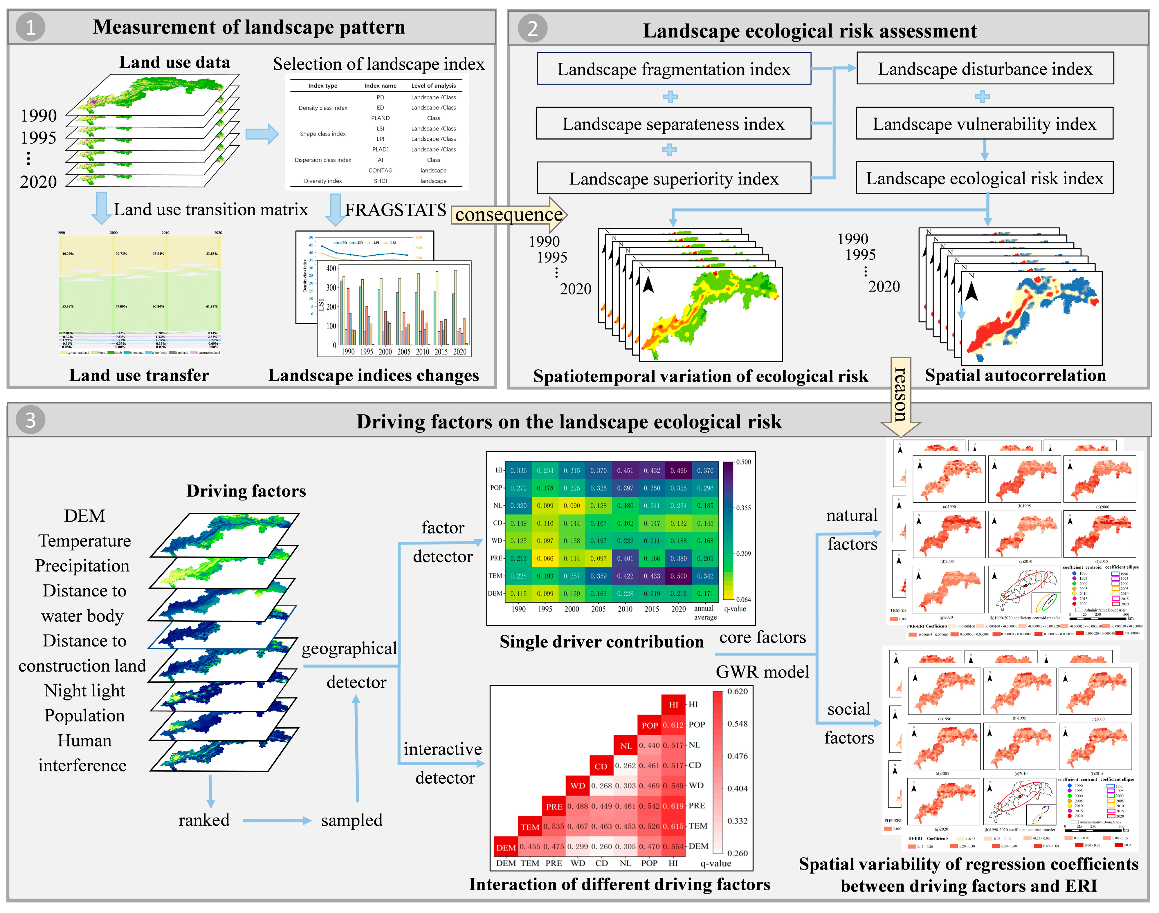
2.3. Research Methodology

This study was conducted based on the following three steps (Figure 2): (1) measurement of landscape pattern, (2) assessment of landscape ecological risk to quantify the consequences of landscape pattern changes, and (3) quantification of the landscape ecological risk drivers in time and space. Each step is described in detail in the following sections.

2.3.1. Land Use Transfer Matrix

The land use transfer matrix includes data on various types of land area at a certain time point in a given region with information on the transfer out and transfer in of various land area types. This reflects the dynamic process of mutual transformation between various types of land area at the beginning and end of a certain period in the region [38,39,40]. The formula is as follows:
S i j = S 11   S 12   S 17 S 21   S 22     S 27    S 71   S 72   S 77
where S is the land area in the study area, 7 is the number of land use types, and i and j are the land type serial numbers at the beginning and end of the TGRA study, respectively.

2.3.2. Selection and Calculation of Landscape Indices

Landscape pattern indices comprise highly concentrated information on landscape patterns, which are quantitative indices reflecting the landscape structural composition and spatial configuration characteristics [41]. To determine the size, regularity, fragmentation, and heterogeneity of the landscape, four major landscape index types were selected and analyzed at the landscape and class levels to reflect the landscape pattern characteristics of the TGRA [39,40]. The specific selected landscape indices are detailed in Table 2, and each calculation was run in FRAGSTATS 4.2. The formulas and descriptions of the indices are detailed in Table S1.

2.3.3. Quantification of Landscape Ecological Risk

The Landscape Ecological Risk Index (ERI) is used to establish the link between landscape structure and regional ecological risk, which can quantify the ecological pressure caused by changes in landscape patterns [5,19,42]. Meanwhile, using risk cells as assessment units is an effective method to assess ERI [10,34]. In this study, the TGRA was divided into 4028 risk units with a 4 km × 4 km scale based on previous studies and the actual situation in the TGRA [11,33]. The “loss and probability cumulative multiplication” paradigm was used to construct the ERI. The formula for calculating ERI is as follows:
E R I = i = 1 n A k i A k R i
where E R I is the landscape ecological risk index of a risk cell, n is the number of land use types, A k is the total area of a risky cell, A k i is the area of the land use type i in a risk cell, and R i is the landscape loss index of the land use type i . The calculation method of R i is shown in Table 3.

2.3.4. Spatial Autocorrelation Analysis

Spatial autocorrelation refers to the potential interdependence of geographic variables within a distribution area; the closer the spatial location, the stronger the correlation. We calculated Global Moran’s I to determine whether the landscape ecological risk exhibited statistical aggregation or dispersion; the significance of Moran’s I was assessed using z-scores [34,35]. The hotspot analysis tool (based on G i * ) was employed to spatially explore the aggregation and clustering patterns of the high or low ERI values and reveal the mechanism of spatial correlation among ERI [43,44]. The specific formulas are as follows:
G l o b a l   M o r a n s   I = i = 1 n j i n W i j X i X ¯ X j X ¯ S 2 i = 1 n j i n W i j  
S 2 = 1 n i = 1 n X i X ¯ 2
Z = I E I V A R I
G i * = j = 1 n W i j X j j = 1 n X j
where n is the number of samples, W i j is the spatial weight matrix, and X i and X j are the attribute values of risk cells i and j, respectively. I > 0 indicates that the ERI exhibits aggregation; I < 0 indicates that the ERI is dispersed; I = 0 indicates that the ERI is randomly distributed in space. E I and V A R I are the mathematical expectation and variance of M o r a n s   I , respectively. Z > 2.58 or Z < −2.58 indicates a significant spatial autocorrelation in the ERI with 99% confidence. G i * represents the aggregation index of patch i.

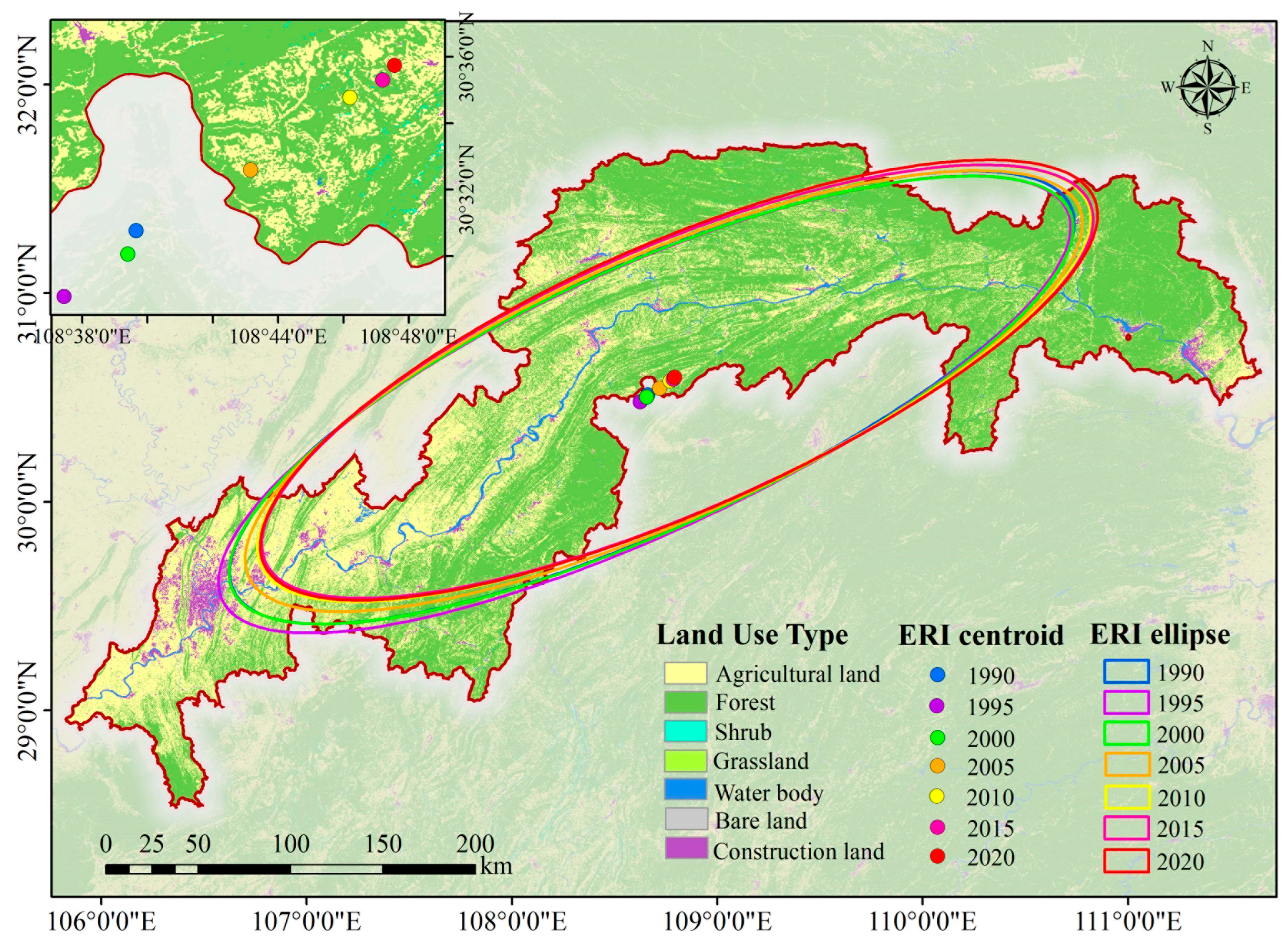
2.3.5. Standard Deviation Ellipse

The standard deviation ellipse can reflect the general outline and distribution direction of spatial organization; an offset ellipse center reflects an offset trend in the spatial center [42,45]. Dynamic offset trajectory was used to assess the shift in the gravity center of the landscape ecological risk and the influence of driving factors on landscape ecological risk. The formulas are as follows:
t a n θ = i = 1 n x i 2 i = 1 n y i 2 + i = 1 n x i 2 i = 1 n y i 2 + 4 i = 1 n x i y i 2 2 i = 1 n x i y i
φ x = 1 n i = 1 n x i c o s θ y i s i n θ 2
φ y = 1 n i = 1 n y i c o s θ x i s i n θ 2
where φ x and φ y represent the standard deviation of the x-axis and y-axis, respectively, x i and y i represent the deviation of the coordinate point of each point-like element from its mean center respectively, θ represents the ellipse rotation angle, and n represents the total number of risk cells.

2.3.6. Selection and Calculation of Driving Factors

Multicollinearity refers to the phenomenon that independent variables are highly correlated with each other. When the variance inflation factor (VIF) is >7.5, the multicollinearity among the drivers is significant [28,46,47] and will cause the contribution of the driver to be inaccurate. Therefore, per related studies [11,34,35], and considering the actual situation of the TGRA, including the rugged topography [48], massive migration [31,49], dramatic climate fluctuations [50,51], and significant land use changes [52,53], eight driving factors were selected. Moreover, the VIF was calculated to avoid multicollinearity among the driving factors. These factors included the following natural factors: DEM, TEM, PRE, distance to water body (WD), and distance to construction land (CD), and the following social factors: NL, POP, and human interference (HI). The driving effects of landscape ecological risk were then analyzed. Among them, WD and CD represent the distances of each evaluation unit from a water body/construction land, respectively, which are raster data with a 30 m resolution. We used the Euclidean Distance tool from ArcGIS to estimate these distances based on land use data. The formula for assigning HI to a risk cell is as follows [3]:
H I = i = 1 m H I i S i S
where H I is the human interference degree of a risk cell, H I i is the disturbance index of i landscape type, S i is the area of i landscape type, and S is the total area of a risk cell.

2.3.7. Geographical Detector

Geographical detector is a statistical method to measure spatial differentiation and reveal the driving forces in natural and social factors [3]. The associated Factor detection module can quantitatively identify the contribution of each driver to landscape ecological risk, while the interactive detection module can evaluate the combined effect of the two drivers [11,54]. To apply the geographical detector, the eight driver factors must first be ranked; the q value of each ERI driver is then obtained based on the classification. The formula is as follows:
q = 1 h = 1 m N h δ h 2 N δ 2
where δ h 2 represents the discrete variance of ERI, h = 1,…, m represents the stratification of all variables, N h represents the number of risk cells in each stratification h, N is the total number of risk cells, and δ 2 is the total variance of the region. The larger the value of q∈[0, 1], the higher its contribution to the landscape ecological risk.

2.3.8. Geographically Weighted Regression (GWR) Model

The GWR model presents the parameters of each geographic location through local regression and generates regression coefficients that vary with geographical location. It spatializes local relationships and better determines the responses between variables in each geographical location [26,28]. Therefore, we used the GWR model to explore the spatially nonstationary correlation between drivers and landscape ecological risks using the following formula:
y i = β 0 u i , v i + k = 1 p β k u i , v i x i k + ε i
where y i is the landscape pattern index, u i , v i is the coordinate of the sampling point i, β 0 u i , v i is the intercept term, β k u i , v i is the kth regression coefficient at point i, p is the number of drivers, x i k is the value of the explanatory variable x k at point i, and ε i is the random noise term.
The adjusted R2 and standard residual are often used to verify the performance of the GWR model [26,55]. Our results showed that the GWR model adjusted R2 was >0.73, indicating a good fit. Moreover, the standard residual in the study area were approximately between −2.5 and 2.5, indicating that the results calculated by the GWR model were reliable.

3. Results

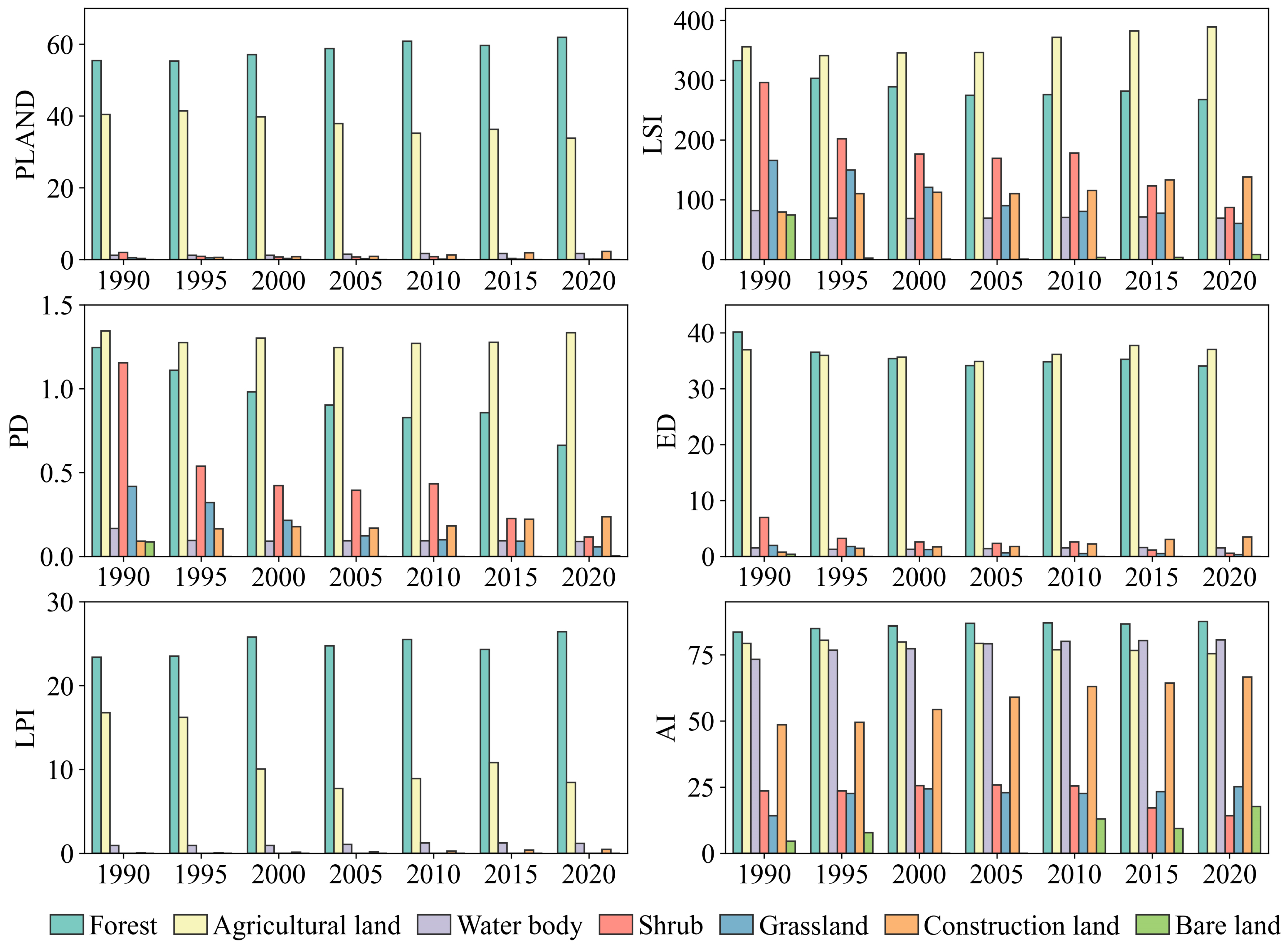
3.1. Landscape Pattern Characteristics

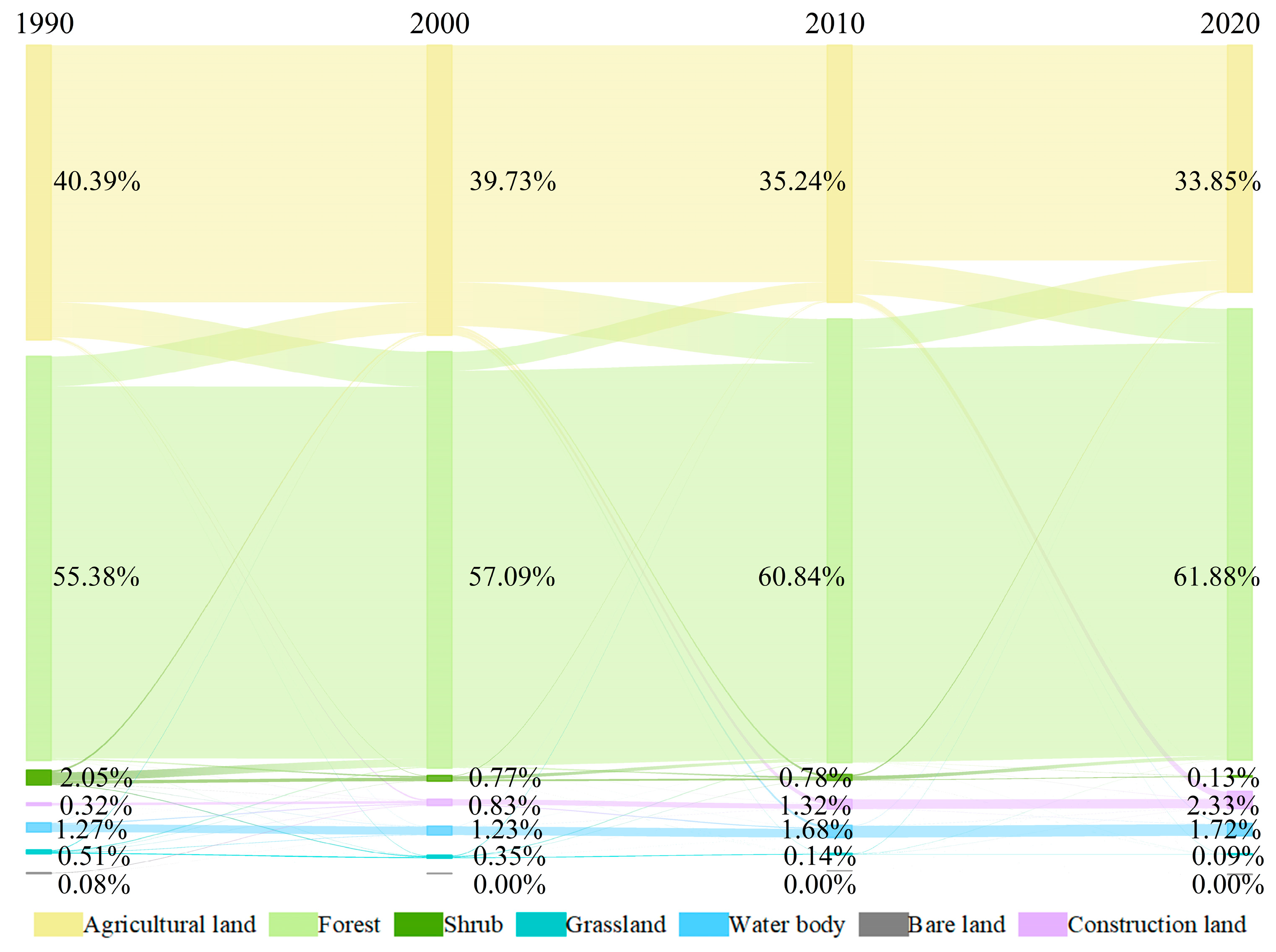
3.1.1. Land Use Transfer

The study period from 1990 to 2020 was divided into three phases to understand the change in land use transfer over the past 30 years of the TGRA (Figure 3). The main land use types of the TGRA were agricultural land and forests, accounting for more than 90% of the area. In the past 30 years, the agricultural land area has continued to decline, from 40.39% in 1990 to 33.85% in 2020, contributing to a total decrease of 3819.62 km2. In addition, the forest area increased to 3796.26 km2 in 30 years. During the study period, the growth rates of construction land in the three phases were 159.38%, 59.04%, and 76.52%, respectively, with a total 1173.92 km2 increase in 30 years. Among the increased construction land area, 41.49%, 94.30%, and 93.09% came from the transfer of agricultural land in the three phases, respectively. Moreover, the water body area expanded by 266.64 km2 from 2000 to 2010 due to the construction of the TGP and water storage. From 1990 to 2020, the main land-use changes were characterized by a significant reduction in agricultural land and expansion of forests, construction land, and water body area.

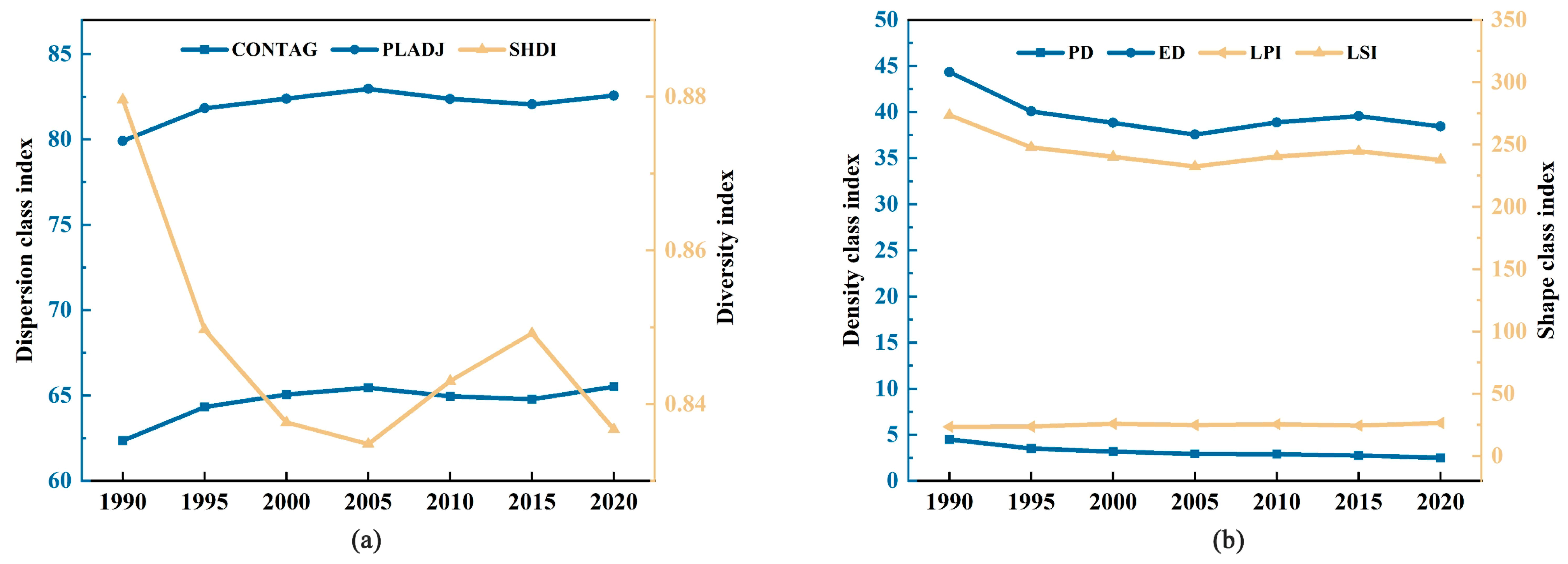
3.1.2. Landscape Index Change

At the landscape level, the changes in the landscape indices of the TGRA from 1990 to 2020 are shown in Figure 4. The proportion of like adjacencies index and contagion index exhibited an overall upward trend, indicating that the landscape in this area formed a good connection between the patches and increased the degree of landscape aggregation. The decrease in the patch density index, edge density index, and landscape shape index indicated that the number of patches per unit area of the landscape decreased, the boundary length was shortened, and the patch shape tended to be regular. The largest patch index rose slightly over 30 years, reflecting the increased dominance of the largest patch and a slight increase in the impact on landscape patterns. The decrease in the Shannon’s diversity index represents uneven landscape development. Hence, it can be inferred that, in the past 30 years, the landscape of the TGRA has tended to develop toward a pattern of increased aggregation, regular shape, and uneven distribution.
At the class level, analyzing a set of landscape indices can better describe the structural dynamics of the landscape type (Figure 5). Over the past 30 years, the landscape types have exhibited different landscape pattern changes. Regarding agricultural land, the percentage of landscape index and largest patch index exhibited an overall downward trend, indicating that the agricultural land area and the landscape advantage decreased. The increase in landscape shape index and decrease in aggregation index reflected the development of agricultural land in the direction of a complex shape and spatial fragmentation. For forests, the percentage of landscape index increased, while the patch density index and landscape shape index exhibited a decreasing trend, indicating that the shape of the patches while expanding tended to be smooth. The adjacent patches showed interconnected patch-like development; the increased aggregation index was primarily attributed to the shrinking public boundary. In the case of construction land, the patch density index, edge density index, and landscape shape index increased with the increasing percentage of landscape index. This observation indicated that the construction land area expansion relied primarily on the increase in the number of patches, which filled in the gaps between patches, enhancing their connectivity and increasing the aggregation index of the construction land.

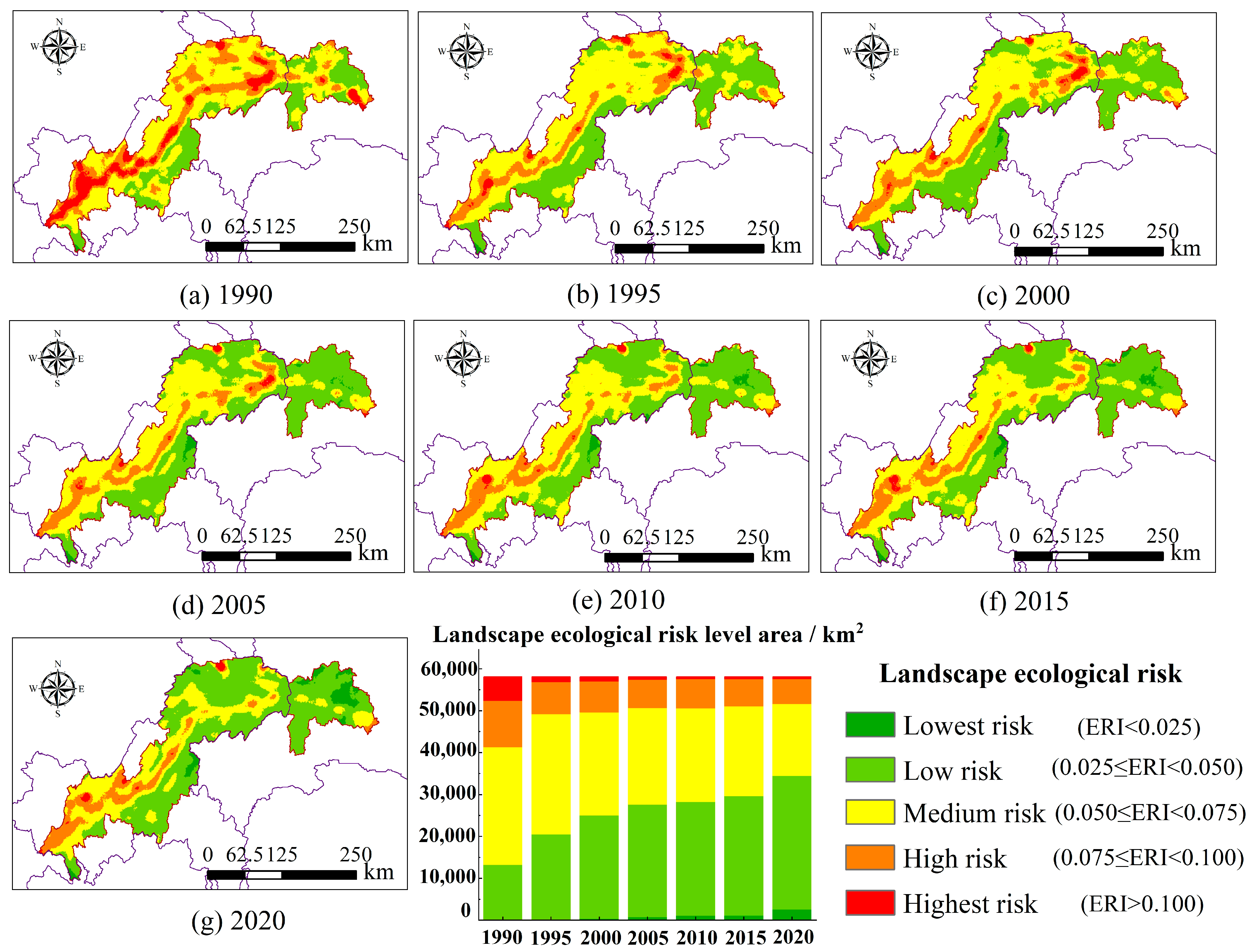
3.2. Landscape Ecological Risk Characteristics

This study used the ERI to characterize the temporal and spatial characteristics of landscape ecological risk to characterize further the risk consequences caused by landscape pattern changes. Based on relevant studies [10,18] and the distribution characteristics of ERI, the landscape ecological risk of the TGRA was standardized and categorized into five levels using the equal interval method, namely, the lowest (ERI < 0.025), low (0.025 ≤ ERI < 0.050), medium (0.050 ≤ ERI < 0.075), high (0.075 ≤ ERI < 0.100), and highest (ERI ≥ 0.100) risk areas.

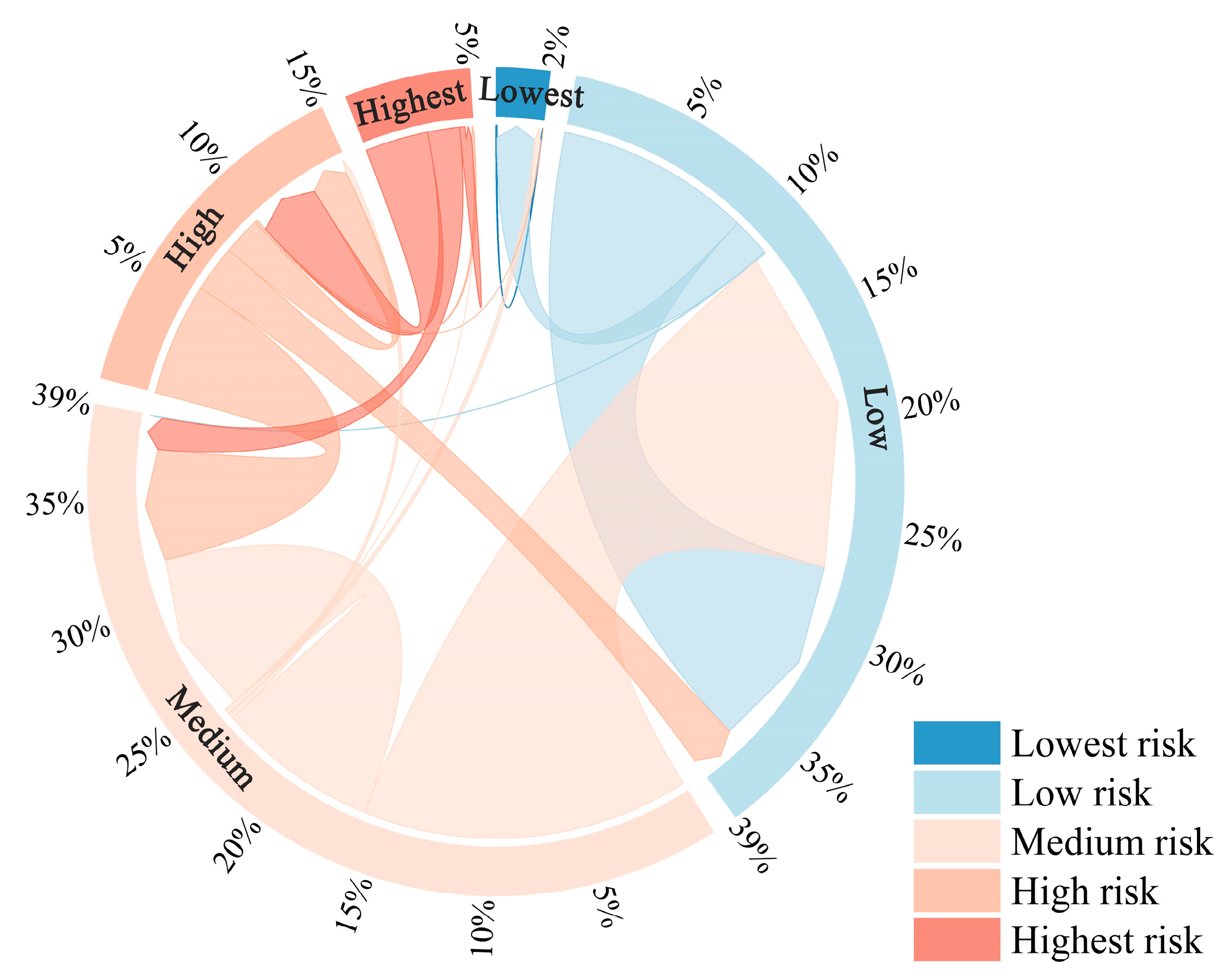
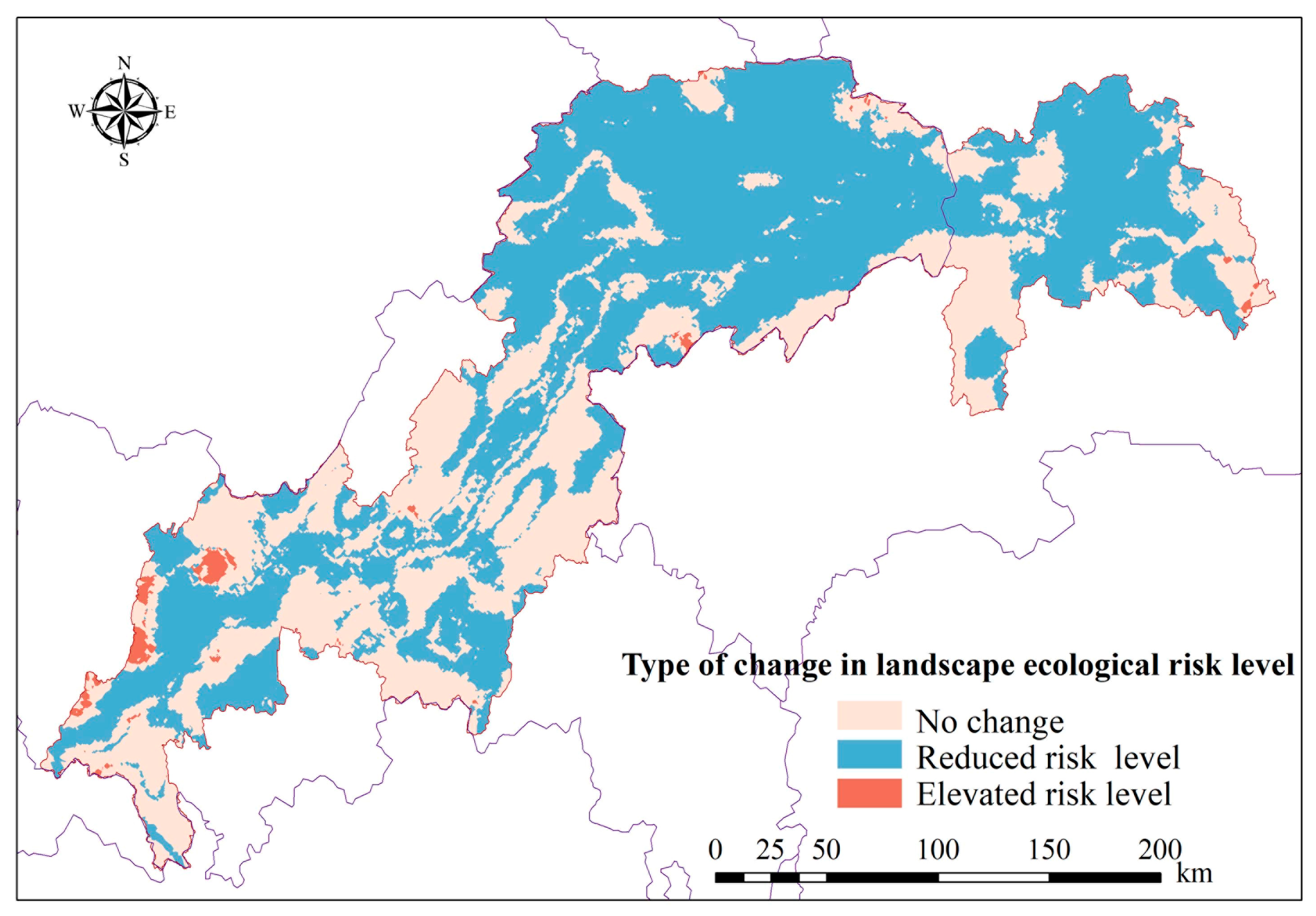
3.2.1. Spatiotemporal Changes of Landscape Ecological Risk

During the study period, the landscape ecological risk level exhibited spatial distribution characteristics that were relatively low east of the TGRA, relatively high west of the TGRA, and relatively high along the Yangtze River (Figure 6). Forests dominated the eastern part of the TGRA with lower landscape ecological risk. The areas with relatively high landscape ecological risk levels were concentrated primarily in the intensive construction land area and along the Yangtze River. It was mainly distributed in the urban economic circle centered on Chongqing, with a high degree of landscape disturbance due to land development and frequent human activities, such as urbanization, construction, and agricultural production activities. Given the cutting by the Yangtze River and its tributaries, the landscape in this region is highly fragmented, with a high landscape ecological risk level.
Overall, the landscape ecological risk in the TGRA exhibited a decreasing trend from 1990 to 2020; the area of the lowest risk and low-risk landscape ecology increased by 2486.84 km2 and 18775.58 km2, respectively. Meanwhile, the areas of medium risk, high risk, and highest risk decreased by 10917.48 km2, 5132.05 km2, and 5212.88 km2, respectively (Figure 6). The landscape ecology risk levels were transformed primarily to the subsequent lower risk level, among which highest risk, high risk, medium risk, and low risk were transferred to 3540.49 km2, 2558.81 km2, 18421.90 km2, and 2173.97 km2, respectively (Figure 7). The risk level reduction area accounted for 60.13% of the total TGRA, mainly located east of the TGRA and the northern portion of the TGRA middle region (Figure 8). Although forests dominate this area, the construction land continuously encroached on the surrounding agricultural land with the accelerating urbanization process; hence, the landscape disturbance degree increased. Therefore, the landscape ecological risk levels were elevated around the main urban area.
The ERI centroid and standard deviation ellipse in the TGRA from 1990 to 2020 are shown in Figure 9. Overall, the ERI centroid showed a spatial transfer pattern of “first to the southwest, then to the northeast,” with the centroid shifting 15.59 km to the northeast. This resulted in a gradual loss of the flattened ERI standard deviation ellipse, an increase in the short axis length, and a decrease in the long axis. These findings indicated that the ecological risk of the TGRA landscape was extended in the short-axis direction and reduced in the long-axis direction. The standard deviation of the elliptical long axis shortened significantly from 1995 to 2010, particularly in the southwest, indicating that the landscape ecological risk west of the TGRA was more concentrated with a faster risk reduction rate. Between 1990 and 1995, the ERI north of the TGRA decreased significantly, shifting the ERI centroid toward the west of the TGRA, where there was less forest and higher landscape ecological risk. From 1995 to 2020, the ERI centroid shifted 20.61 km to the northeast, possibly due to the transformation of a large amount of agricultural land in the southwest into forests, thus improving the ecological condition and leading to the ERI centroid moving to the northeast.

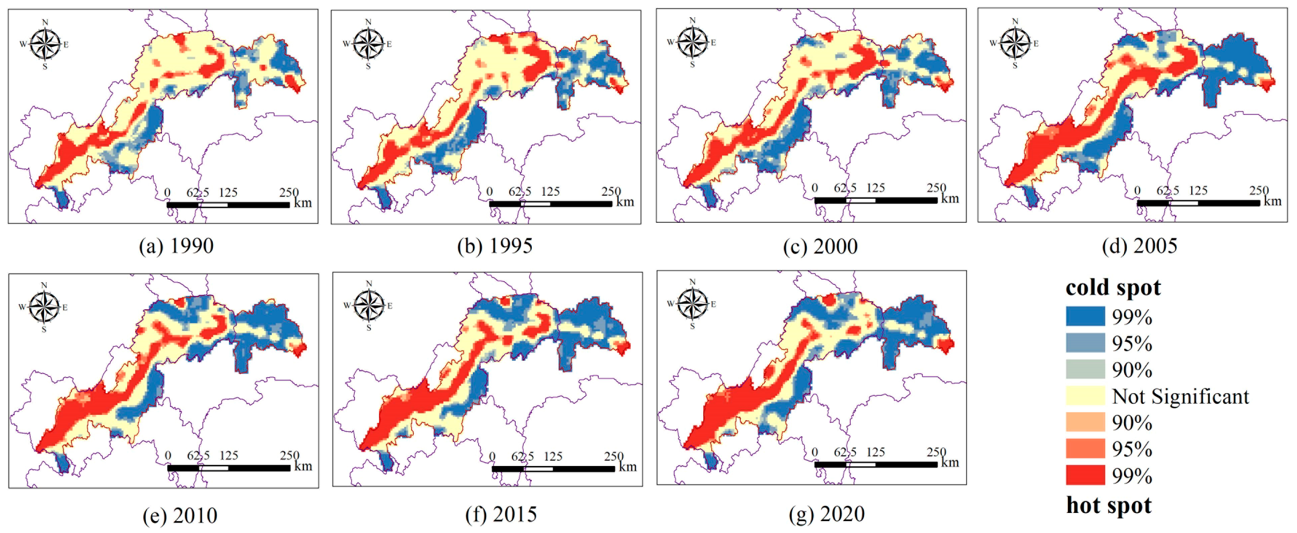
3.2.2. Spatial Autocorrelation of Landscape Ecological Risk

Based on the ERI of each risk cell, the Global Moran’s I of the landscape ecological risk was calculated from 1990 to 2020. A Global Moran’s I > 0 showed an initial decreasing trend followed by an increasing trend, and the z-score of the normal statistics was > 2.58 (Table 4). This indicated that the TGRA landscape ecological risk exhibited significant spatial aggregation, and the spatial correlation of the landscape ecological risk continued to increase after 2000.
Over the past 30 years, the spatial distribution of ERI in the TGRA showed a gradient distribution pattern of decreasing along both sides of the Yangtze River. Figure 10 shows an expansion in the hot spot and cold spot ranges of the landscape ecological risk as well as smaller areas without significant changes. This indicates that, with the decrease in the landscape ecological risk, the difference between ERI values gradually decreased, and the spatial correlation increased. The cold spots were distributed primarily in the zone far from the Yangtze River and were dominated by large forest areas; these spots continued to increase with the aggregated forest expansion. In comparison, the hot spots were concentrated primarily in the west of the TGRA and the river valley along the Yangtze River. These areas involved dense human activities of construction land and agricultural land; hence, the spatial correlation gradually increased and expanded with the transfer of land use and its characteristic changes. By 2020, the original strip-like hot spots spread in a doughnut shape west of the TGRA.

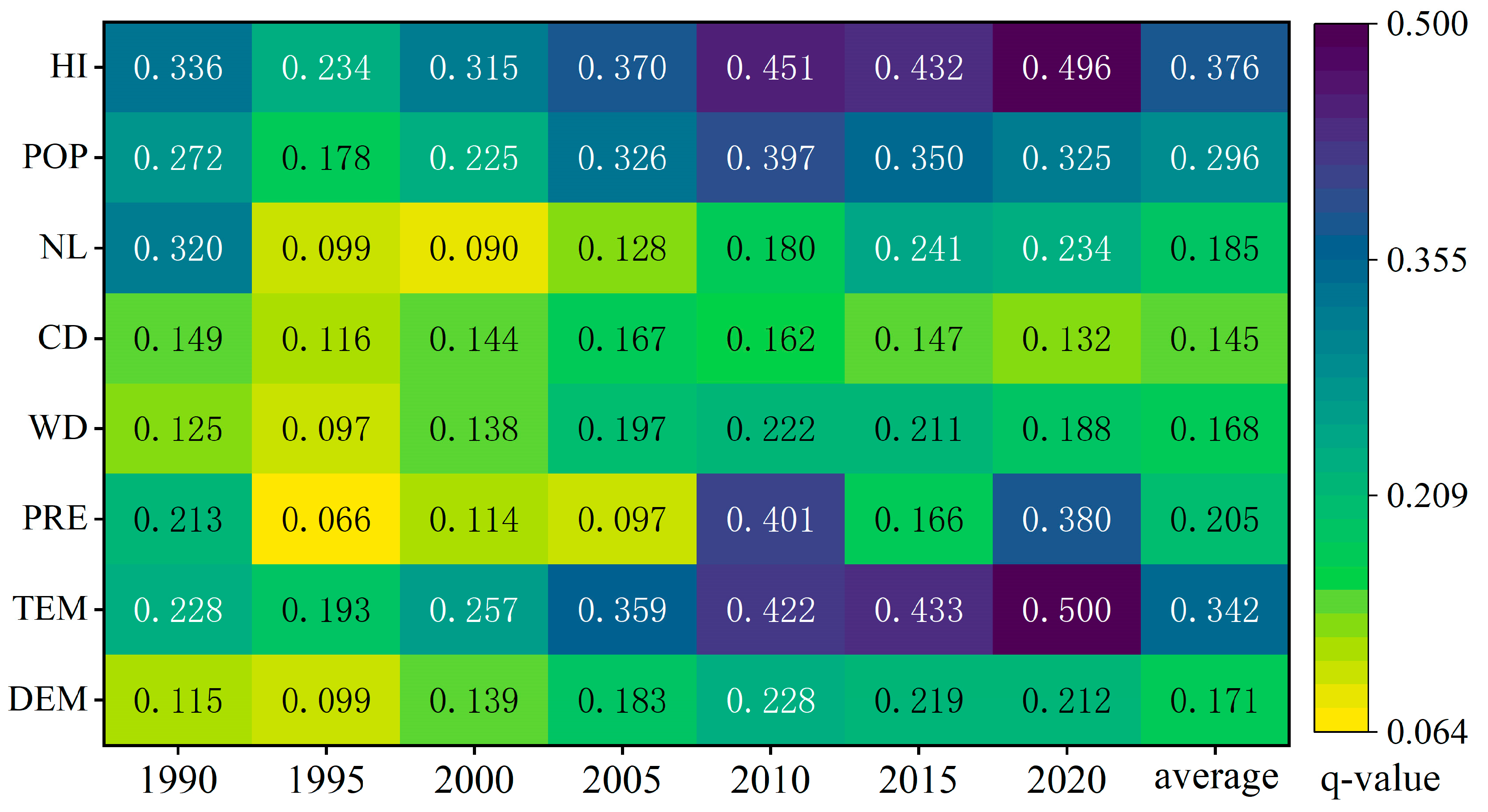
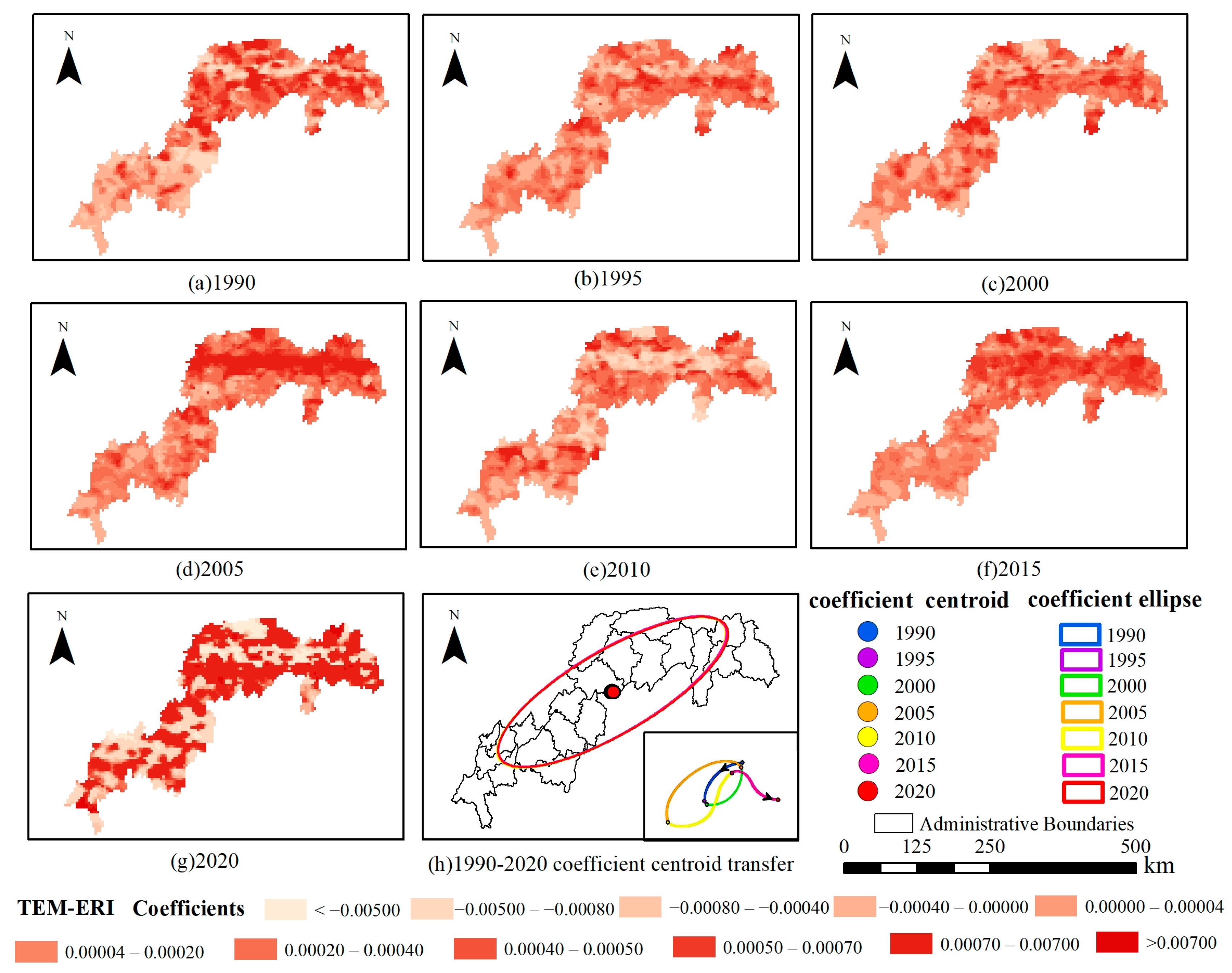
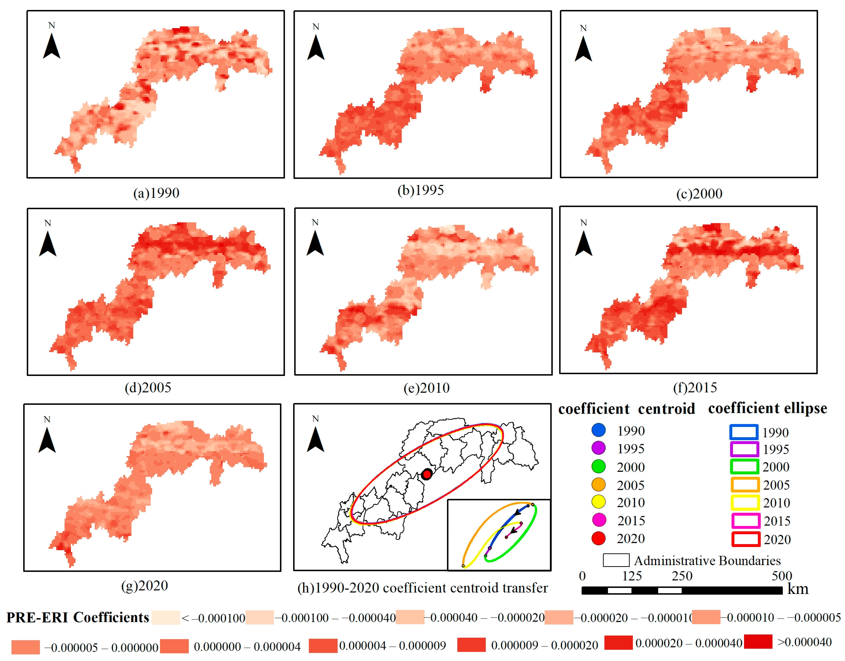
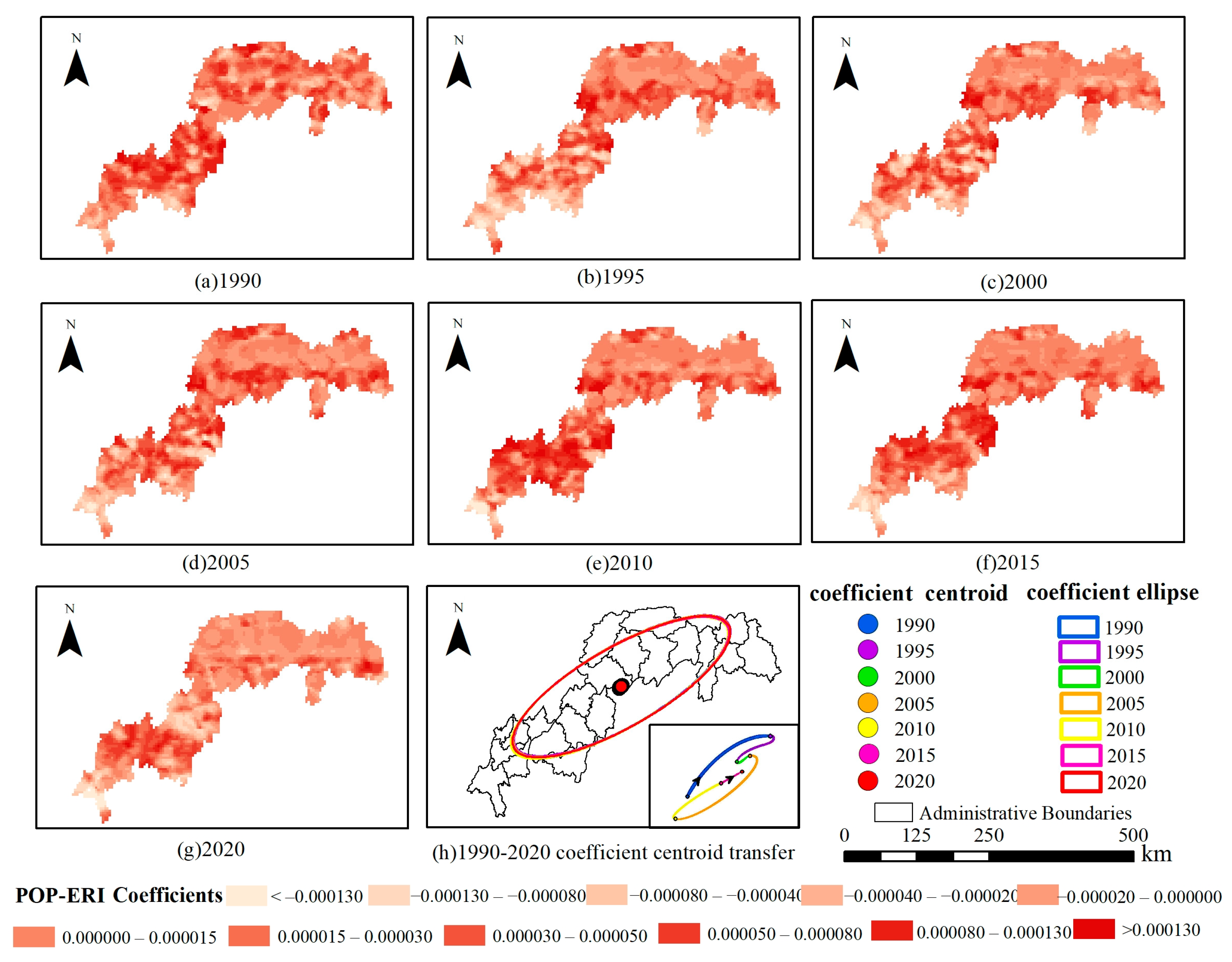
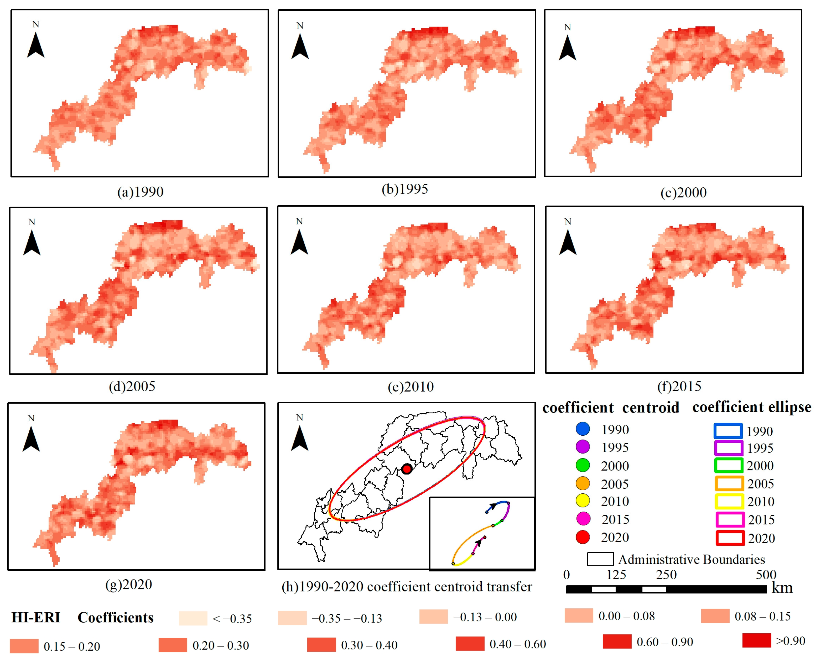
3.3. Analysis of Landscape Ecological Risk Driving Factors

As per the results of the geographical detector, the TGRA landscape ecological risk was influenced by natural and social factors, and the contribution rate of different drivers to landscape ecological risk varied significantly. The eight drivers selected in this paper contributed increasingly to the landscape ecological risk over the 30-year period (Figure 11). Among the social factors, human interference and population density had stronger contribution rates to landscape ecological risk. Human interference was the predominant contributor with an average contribution rate >0.37, which tended to increase yearly, indicating that human activities had a greater impact on landscape ecological risk, and the degree of impact gradually increased. Among the natural factors, annual precipitation and average temperature, as essential factors for vegetation growth, influenced the ecological risk changes in the landscape with high contributions to landscape ecological risk. The contribution of annual average temperature increased rapidly and surpassed human interference in 2020, indicating that the influence of annual average temperature on landscape ecological risk is important.
The interaction detection results (Figure 12) showed a two-factor interaction enhancement in the contribution of the factor interactions to the landscape ecological risk during the study period. This indicated that the driving factors were dependent on each other. The interaction between human interference and annual average temperature made the largest contribution to the landscape ecological risk, reaching ≥ 0.46 and exhibiting a fluctuating increasing trend. This indicated that human interference and annual average temperature were important factors affecting landscape ecological risk, and their degree of influence gradually increased. Most significant interactions were observed between human interference and other factors, likely because the relationships between other driving factors and human socio-economic activities, such as urbanization and cultivation, were more complex. In addition, the disturbance effect on the landscape ecological risk of the TGRA was stronger under the background of rapid socio-economic development.

4. Discussion

4.1. Landscape Pattern and Landscape Ecological Risk Change Characteristics

Regarding landscape pattern change characteristics, the area of agricultural land in the TGRA has gradually decreased. Meanwhile, fragmentation has increased over the 30-year study period, which agrees with the findings of previous studies [56,57]. Moreover, the area of forests continued to increase along with the degree of aggregation. However, the area of construction land grew at a faster rate, with aggravated patches. These observations were consistent with the findings of Zhang [58]. Regarding the spatial and temporal distribution of landscape ecological risks, the areas (distributed in strips) along the Yangtze River exhibited relatively high landscape ecological risk levels. This was due primarily to most of the cities being distributed in the valley of the Yangtze River mainstream below 300 m elevation with relatively flat terrain, sufficient water supply, developed agriculture, and high population density [59]. Thus, a high degree of landscape disturbance occurred in these areas. From 1990 to 2020, the TGRA landscape ecological risk showed a decreasing trend [33,60,61]. The areas with forests exhibited lower risk levels due to the implementation of a series of ecological protection policies, including returning farmland to forest, which effectively increased the forest area, improved the connectivity of the forest, and enriched the ecology of these areas.
Moreover, due to the construction and impoundment of the TGP, large amounts of agricultural land along the Yangtze River with high ERI values have been flooded, causing the area with a relatively high landscape ecological risk to present a downward trend [31]. The rapid development of urbanization has led to an intensive expansion of construction land and the development of construction land toward aggregation. This reduced ERI values in the highest-risk areas dominated by construction land. However, the landscape ecology in the main urban areas of Chongqing and the middle of the TGRA continued to face more significant risks, confirming the views of He [33].

4.2. Spatial Response of Landscape Ecological Risk to Drivers

The results of the geographical detector showed that human interference, annual average temperature, population density, and annual precipitation were the core factors influencing the landscape ecological risk. Since the geographical detector did not reflect the spatial differences in driving factors, these characteristics were captured using the GWR model.
The GWR coefficients illustrated the spatially heterogeneous response of landscape ecological risk to drivers, providing additional details regarding the spatial relationship between landscape ecological risk and various drivers. Figure 13 and Figure 14 show the regression coefficient results of ERI with annual average temperature and annual precipitation, respectively. We found that annual average temperature and ERI were strongly correlated. Areas with frequent landscape-type transitions at the junction generally exhibited negative correlations, while the study area generally exhibited positive correlations; landscape ecological risk increased with an increase in temperature. This may be due to higher temperatures causing increased forest instability and tree mortality rates [62,63]. This further increases the degree of forest loss and the ecological risk to the landscape, demonstrating the negative impact that global warming can have on ecosystems. The impact of annual precipitation on ERI fluctuates greatly, with a larger area and probability of negative correlation in the east of the TGRA. This is likely due to the wider distribution of forests east of the TGRA. Hence, the increase in precipitation may have led to increased vegetation cover [64], thus expanding the forest land range, increasing the degree of landscape aggregation, and decreasing ERI. In contrast, the annual precipitation and ERI exhibited a higher probability of positive correlation in the west of the TGRA. This may be due to the large proportion of agricultural land and construction land located west of the TGRA. Moreover, this region is highly sensitive to precipitation as the impervious surface affects precipitation infiltration, causing it to be greatly impacted by natural disasters. More specifically, increased precipitation may lead to flood disasters, increased landscape loss, and higher ERI, which agrees with previous research results [65].
The results presented in Section 3.2 showed that urbanization expanded and agglomerated the landscape into patches during economic development. With an increase in the aggregation index of construction land, the ERI decreased, suggesting that the urbanization process may reduce the ecological risk of the landscape, confirming the view of Yang [26]. However, this does not necessarily imply that urbanization is ecologically beneficial. The results of the geographical detector showed that population density and human interference strongly impacted the landscape ecological risk. Meanwhile, the GWR model suggested that the effects of population density and human interference on ERI were positively correlated in most areas (Figure 15 and Figure 16). Zou [66] and Wang [67] found that high population concentration and disturbance negatively affected the landscape structure and ecological environment. Moreover, they found that increased population concentration caused the expansion of towns and industrial activities, leading to stronger landscape disturbance and higher ERI. These findings were likely due to the GWR model considering only the changes of drivers in space while being limited in the reflection of time.
Concerning the dynamic change in the coefficient centroid, obvious regional differences were observed in the direction and degree of the landscape ecological risk response to each driver (Figure 13, Figure 14, Figure 15 and Figure 16). Hence, the response of landscape ecological risk to driving factors was a comprehensive response to a series of conditions, including various natural and social factors. The two-factor enhancement effect of the geographical detector demonstrated the interactions between the driving factors. For example, population density is large in areas with high human interference, and the resulting urban heat island effect increases the annual average temperature in the area. In addition, the landscape ecological risk is increased under the combined effect of the three factors. The GWR coefficient centroid further indicated that the direction of movement is more similar in natural factors (annual average temperature and annual precipitation) or social factors (population density and human interference). This is because the interaction between social or natural factors is simpler than between the two types of impact factors, and the driving force of landscape ecological risk is more consistent. However, the transfer of the coefficient centroid of natural factors was relatively disordered, indicating that annual average temperature or annual precipitation may indirectly affect landscape ecological risk by acting on other factors, and the driving mechanism for landscape ecological risk may be more complex.
The GWR model can intuitively reveal the spatial difference characteristics of the correlations between each driver and landscape ecological risk. This suggests that decision-makers can form targeted decisions on landscape ecological risk management in localized areas based on our findings. For example, given that annual average temperature showed a positive correlation with ERI in non-junction areas, in areas with more forests, such as east of the TGRA, decision-makers can reduce the surface temperature by altering the structure of forest stands to reduce the landscape ecological risk [68,69]. Although the negative ecological impact caused by human activities is often inevitable, our study found that urban agglomerative expansion can control landscape ecological risk. There are also related studies showing that regular cities are beneficial to ecosystem health [26,70]. Therefore, decision-makers can start from the urban expansion mode to guide the intensive development of cities to reduce the ecological risk of urban landscapes.

4.3. Limitations and Generalized Contributions

In this study, the contribution to landscape ecological risk was insufficient due to the limited selection of drivers and their complex interactions. Therefore, additional drivers, such as biomass, vegetation cover, etc., should be considered in further studies. Moreover, the GWR model only models the parameters spatially. Thus, further work is needed to determine the temporal and spatial differences in the effects of drivers on landscape ecological risk. This study analyzed the landscape ecological risk characteristics and their drivers’ contributions under a long-term time series, providing more empirical support for its regulations and improving the reliability of the results. In addition, this study extended the exploration of the GWR model and its transfer of coefficient centroid in landscape ecological risk. It also provided more spatial details regarding the impacts of drivers on landscape ecological risk and clarified the localized contributions of drivers. Moreover, this model compared the interrelationships among different drivers and provided deeper insights into the driving mechanisms of landscape ecological risk, which are rarely discussed in the literature. In summary, this study broadens the concepts surrounding landscape ecological risks and their driving factors and provides a more targeted decision strategy for ecological risk management.

5. Conclusions

This study investigated the spatial and temporal changes in landscape ecological risk and its driving factors in the TGRA from 1990 to 2020 and attempted to understand the spatial differentiation in the impacts of natural and social factors on landscape ecological risk. Our results showed that: (1) From 1990 to 2020, the agricultural land decreased, while forest and construction land expanded in the TGRA. The overall landscape pattern shifted toward aggregation. (2) The landscape ecological risk in the TGRA over the past 30 years exhibited a decreasing trend. The areas with relatively high landscape ecological risk were concentrated primarily in the main urban area west of the TGRA and along the Yangtze River, where spatial aggregation was obvious. (3) Social and natural factors affected landscape ecological risk. The main driving factors were human interference, annual average temperature, population density, and annual precipitation. Moreover, interactions were detected between the drivers. (4) The influence of driving factors on landscape ecological risk showed spatial heterogeneity. Spatially, the influence of social factors (human interference and population density) on landscape ecological risk was predominantly positively correlated. Meanwhile, the influence of natural factors (annual average temperature and annual precipitation) on landscape ecological risk varied widely in spatial distribution, and the driving mechanisms were more complex. Collectively, this study extends the exploration of the driving mechanisms in landscape ecological risk. The framework offers deeper insights into the landscape ecological risk changes and drivers. In the future, we will focus on the changes and development of landscape patterns in different scenarios and provide relevant suggestions for ecological risk control and ecological protection decision-making.

Supplementary Materials

The following supporting information can be downloaded at https://www.mdpi.com/article/10.3390/rs15194884/s1, Table S1: The formula and meaning of landscape indices.

Author Contributions

Conceptualization, Z.Y.; methodology, Z.Y. and Z.W.; validation, Z.Y. and C.Z.; formal analysis, Y.W. (Yunqi Wang); resources, Y.W. (Yunqi Wang) and Y.W. (Yujie Wang); data curation, Z.W. and Y.L.; writing—original draft preparation, Z.Y.; writing—review and editing, Y.W. (Yunqi Wang), Y.W. (Yujie Wang) and Z.W.; visualization, Z.Y.; supervision, Y.W. (Yunqi Wang); project administration, Y.W. (Yunqi Wang) and Y.W. (Yujie Wang). All authors have read and agreed to the published version of the manuscript.

Funding

This research was funded by the Major Science and Technology Projects of the Ministry of Water Resources (SKS-2022082) and the Research on Monitoring Technology of Chongqing Carbon Sequestration Based on Remote Sensing Technology (CSTB2022TIAD-KPX0202).

Data Availability Statement

The data are not publicly available due to the policy of the institute.

Conflicts of Interest

The authors declare no conflict of interest.

References

  1. Fang, X.; Li, J.; Ma, Q. Integrating green infrastructure, ecosystem services and nature-based solutions for urban sustainability: A comprehensive literature review. Sustain. Cities Soc. 2023, 98, 104843. [Google Scholar] [CrossRef]
  2. Lafortezza, R.; Sanesi, G. Nature-based solutions: Settling the issue of sustainable urbanization. Environ. Res. 2019, 172, 394–398. [Google Scholar] [CrossRef] [PubMed]
  3. Karimian, H.; Zou, W.; Chen, Y.; Xia, J.; Wang, Z. Landscape ecological risk assessment and driving factor analysis in Dongjiang river watershed. Chemosphere 2022, 307, 135835. [Google Scholar] [CrossRef] [PubMed]
  4. Yang, M.; Shi, L.; Liu, B. Risks assessment and driving forces of urban environmental accident. J. Clean. Prod. 2022, 340, 130710. [Google Scholar] [CrossRef]
  5. Qian, Y.; Dong, Z.; Yan, Y.; Tang, L. Ecological risk assessment models for simulating impacts of land use and landscape pattern on ecosystem services. Sci. Total Environ. 2022, 833, 155218. [Google Scholar] [CrossRef] [PubMed]
  6. Hope, B.K. An examination of ecological risk assessment and management practices. Environ. Int. 2006, 32, 983–995. [Google Scholar] [CrossRef]
  7. Lal, P.; Shekhar, A.; Kumar, A. Quantifying Temperature and Precipitation Change Caused by Land Cover Change: A Case Study of India Using the WRF Model. Front. Environ. Sci. 2021, 9, 766328. [Google Scholar] [CrossRef]
  8. Yue, Y.; Geng, L.; Li, M. The impact of climate change on aeolian desertification: A case of the agro-pastoral ecotone in northern China. Sci. Total Environ. 2023, 859, 160126. [Google Scholar] [CrossRef]
  9. Nesshöver, C.; Assmuth, T.; Irvine, K.N.; Rusch, G.M.; Waylen, K.A.; Delbaere, B.; Haase, D.; Jones-Walters, L.; Keune, H.; Kovacs, E.; et al. The science, policy and practice of nature-based solutions: An interdisciplinary perspective. Sci. Total Environ. 2017, 579, 1215–1227. [Google Scholar] [CrossRef]
  10. Xu, W.; Wang, J.; Zhang, M.; Li, S. Construction of landscape ecological network based on landscape ecological risk assessment in a large-scale opencast coal mine area. J. Clean. Prod. 2021, 286, 125523. [Google Scholar] [CrossRef]
  11. Ren, D.; Cao, A. Analysis of the heterogeneity of landscape risk evolution and driving factors based on a combined GeoDa and Geodetector model. Ecol. Indic. 2022, 144, 109568. [Google Scholar] [CrossRef]
  12. Liu, W.; Chang, A.C.; Chen, W.; Zhou, W.; Feng, Q. A framework for the urban eco-metabolism model—Linking metabolic processes to spatial patterns. J. Clean. Prod. 2017, 165, 168–176. [Google Scholar] [CrossRef]
  13. Lee, Y.; Yeh, C.; Huang, S. Energy hierarchy and landscape sustainability. Landscape Ecol. 2013, 28, 1151–1159. [Google Scholar] [CrossRef]
  14. Li, W.; Wang, Y.; Xie, S.; Sun, R.; Cheng, X. Impacts of landscape multifunctionality change on landscape ecological risk in a megacity, China: A case study of Beijing. Ecol. Indic. 2020, 117, 106681. [Google Scholar] [CrossRef]
  15. Mo, W.; Wang, Y.; Zhang, Y.; Zhuang, D. Impacts of road network expansion on landscape ecological risk in a megacity, China: A case study of Beijing. Sci. Total Environ. 2017, 574, 1000–1011. [Google Scholar] [CrossRef] [PubMed]
  16. Wang, H.; Liu, X.; Zhao, C.; Chang, Y.; Liu, Y.; Zang, F. Spatial-temporal pattern analysis of landscape ecological risk assessment based on land use/land cover change in Baishuijiang National nature reserve in Gansu Province, China. Ecol. Indic. 2021, 124, 107454. [Google Scholar] [CrossRef]
  17. Liu, Y.; Peng, J.; Zhang, T.; Zhao, M. Assessing landscape eco-risk associated with hilly construction land exploitation in the southwest of China: Trade-off and adaptation. Ecol. Indic. 2016, 62, 289–297. [Google Scholar] [CrossRef]
  18. Chen, J.; Dong, B.; Li, H.; Zhang, S.; Peng, L.; Fang, L.; Zhang, C.; Li, S. Study on landscape ecological risk assessment of Hooded Crane breeding and overwintering habitat. Environ. Res. 2020, 187, 109649. [Google Scholar] [CrossRef]
  19. Ai, J.; Yu, K.; Zeng, Z.; Yang, L.; Liu, Y.; Liu, J. Assessing the dynamic landscape ecological risk and its driving forces in an island city based on optimal spatial scales: Haitan Island, China. Ecol. Indic. 2022, 137, 108771. [Google Scholar] [CrossRef]
  20. Peng, J.; Xie, P.; Liu, Y.; Ma, J. Urban thermal environment dynamics and associated landscape pattern factors: A case study in the Beijing metropolitan region. Remote Sens. Environ. 2016, 173, 145–155. [Google Scholar] [CrossRef]
  21. Zhang, R.; Li, S.; Wei, B.; Zhou, X. Characterizing Production–Living–Ecological Space Evolution and Its Driving Factors: A Case Study of the Chaohu Lake Basin in China from 2000 to 2020. ISPRS Int. J. Geo-Inf. 2022, 11, 447. [Google Scholar] [CrossRef]
  22. Hou, M.; Ge, J.; Gao, J.; Meng, B.; Li, Y.; Yin, J.; Liu, J.; Feng, Q.; Liang, T. Ecological Risk Assessment and Impact Factor Analysis of Alpine Wetland Ecosystem Based on LUCC and Boosted Regression Tree on the Zoige Plateau, China. Remote Sens. 2020, 12, 368. [Google Scholar] [CrossRef]
  23. Shi, Y.; Feng, C.; Yu, Q.; Han, R.; Guo, L. Contradiction or coordination? The spatiotemporal relationship between landscape ecological risks and urbanization from coupling perspectives in China. J. Clean. Prod. 2022, 363, 132557. [Google Scholar] [CrossRef]
  24. He, J.; Pan, Z.; Liu, D.; Guo, X. Exploring the regional differences of ecosystem health and its driving factors in China. Sci. Total Environ. 2019, 673, 553–564. [Google Scholar] [CrossRef] [PubMed]
  25. Zhou, X.; Wen, H.; Zhang, Y.; Xu, J.; Zhang, W. Landslide susceptibility mapping using hybrid random forest with GeoDetector and RFE for factor optimization. Geosci. Front. 2021, 12, 101211. [Google Scholar] [CrossRef]
  26. Yang, M.; Gao, X.; Zhao, X.; Wu, P. Scale effect and spatially explicit drivers of interactions between ecosystem services—A case study from the Loess Plateau. Sci. Total Environ. 2021, 785, 147389. [Google Scholar] [CrossRef]
  27. Zhao, R.; Zhan, L.; Yao, M.; Yang, L. A geographically weighted regression model augmented by Geodetector analysis and principal component analysis for the spatial distribution of PM2.5. Sustain. Cities Soc. 2020, 56, 102106. [Google Scholar] [CrossRef]
  28. Xue, C.; Chen, X.; Xue, L.; Zhang, H.; Chen, J.; Li, D. Modeling the spatially heterogeneous relationships between tradeoffs and synergies among ecosystem services and potential drivers considering geographic scale in Bairin Left Banner, China. Sci. Total Environ. 2023, 855, 158834. [Google Scholar] [CrossRef]
  29. Xiao, Y.; Xiao, Q.; Xiong, Q.; Yang, Z. Effects of Ecological Restoration Measures on Soil Erosion Risk in the Three Gorges Reservoir Area Since the 1980s. GeoHealth 2020, 4, e2020GH000274. [Google Scholar] [CrossRef]
  30. Luo, X.; Wang, F.; Zhang, Z.; Che, A. Establishing a monitoring network for an impoundment-induced landslide in Three Gorges Reservoir Area, China. Landslides 2009, 6, 27–37. [Google Scholar] [CrossRef]
  31. Xu, X.; Tan, Y.; Yang, G.; Li, H.; Su, W. Impacts of China’s Three Gorges Dam Project on net primary productivity in the reservoir area. Sci. Total Environ. 2011, 409, 4656–4662. [Google Scholar] [CrossRef] [PubMed]
  32. Wang, S.; Zhang, Q.; Wang, Z.; Yu, L.; Xiang, S.; Gao, M. GIS-based ecological risk assessment and ecological zoning in the Three Gorges Reservoir Area. Acta Ecol. Sin. 2022, 42, 4654–4664. [Google Scholar]
  33. He, J.; Wu, L.; Zhang, L.; Zhang, M. Ecological risk assessment of the Three Gorges reservoir landscape based on ecological plots. Ecol. Environ. Monit. Three Gorges. 2022, 7, 11–22. [Google Scholar]
  34. Lin, X.; Wang, Z. Landscape ecological risk assessment and its driving factors of multi-mountainous city. Ecol. Indic. 2023, 146, 109823. [Google Scholar] [CrossRef]
  35. Du, L.; Dong, C.; Kang, X.; Qian, X.; Gu, L. Spatiotemporal evolution of land cover changes and landscape ecological risk assessment in the Yellow River Basin, 2015–2020. J. Environ. Manag. 2023, 332, 117149. [Google Scholar] [CrossRef]
  36. Wang, Z.; Wang, Y.; Ding, X.; Wang, Y.; Yan, Z.; Wang, S. Evaluation of net anthropogenic nitrogen inputs in the Three Gorges Reservoir Area. Ecol. Indic. 2022, 139, 108922. [Google Scholar] [CrossRef]
  37. Yang, J.; Huang, X. The 30 m annual land cover dataset and its dynamics in China from 1990 to 2019. Earth Syst. Sci. Data 2021, 13, 3907–3925. [Google Scholar] [CrossRef]
  38. Cuba, N. Research note: Sankey diagrams for visualizing land cover dynamics. Landsc. Urban Plan 2015, 139, 163–167. [Google Scholar] [CrossRef]
  39. Cao, J.; Li, T. Analysis of spatiotemporal changes in cultural heritage protected cities and their influencing factors: Evidence from China. Ecol. Indic. 2023, 151, 110327. [Google Scholar] [CrossRef]
  40. Zhang, Q.; Chen, C.; Wang, J.; Yang, D.; Zhang, Y.; Wang, Z.; Gao, M. The spatial granularity effect, changing landscape patterns, and suitable landscape metrics in the Three Gorges Reservoir Area, 1995–2015. Ecol. Indic. 2020, 114, 106259. [Google Scholar] [CrossRef]
  41. Jin, H.; Xu, J.; Peng, Y.; Xin, J.; Peng, N.; Li, Y.; Huang, J.; Zhang, R.; Li, C.; Wu, Y.; et al. Impacts of landscape patterns on plant species diversity at a global scale. Sci. Total Environ. 2023, 896, 165193. [Google Scholar] [CrossRef] [PubMed]
  42. Yang, L.A.; Li, Y.; Jia, L.; Ji, Y.; Hu, G. Ecological risk assessment and ecological security pattern optimization in the middle reaches of the Yellow River based on ERI+MCR model. J. Geogr. Sci. 2023, 33, 823–844. [Google Scholar] [CrossRef]
  43. Yang, Y. Evolution of habitat quality and association with land-use changes in mountainous areas: A case study of the Taihang Mountains in Hebei Province, China. Ecol. Indic. 2021, 129, 107967. [Google Scholar] [CrossRef]
  44. Chen, Y.; Wang, J.; Xiong, N.; Sun, L.; Xu, J. Impacts of Land Use Changes on Net Primary Productivity in Urban Agglomerations under Multi-Scenarios Simulation. Remote Sens. 2022, 14, 1755. [Google Scholar] [CrossRef]
  45. Zhang, Y.; Jiang, P.; Cui, L.; Yang, Y.; Ma, Z.; Wang, Y.; Miao, D. Study on the spatial variation of China’s territorial ecological space based on the standard deviation ellipse. Front. Environ. Sci. 2022, 10, 982734. [Google Scholar] [CrossRef]
  46. Wang, Y.; Chen, W.; Kang, Y.; Li, W.; Guo, F. Spatial correlation of factors affecting CO2 emission at provincial level in China: A geographically weighted regression approach. J. Clean. Prod. 2018, 184, 929–937. [Google Scholar] [CrossRef]
  47. Zhang, Y.; Hou, K.; Qian, H.; Gao, Y.; Fang, Y.; Xiao, S.; Tang, S.; Zhang, Q.; Qu, W.; Ren, W. Characterization of soil salinization and its driving factors in a typical irrigation area of Northwest China. Sci. Total Environ. 2022, 837, 155808. [Google Scholar] [CrossRef]
  48. Teng, M.; Huang, C.; Wang, P.; Zeng, L.; Zhou, Z.; Xiao, W.; Huang, Z.; Liu, C. Impacts of forest restoration on soil erosion in the Three Gorges Reservoir area, China. Sci. Total Environ. 2019, 697, 134164. [Google Scholar] [CrossRef]
  49. Hwang, S.; Xi, J.; Cao, Y.; Feng, X.; Qiao, X. Anticipation of migration and psychological stress and the Three Gorges Dam project, China. Soc. Sci. Med. 2007, 65, 1012–1024. [Google Scholar] [CrossRef]
  50. Huang, C.; Zhou, Z.; Teng, M.; Wu, C.; Wang, P. Effects of climate, land use and land cover changes on soil loss in the Three Gorges Reservoir area, China. Geogr. Sustain. 2020, 1, 200–208. [Google Scholar] [CrossRef]
  51. Song, Z.; Liang, S.; Feng, L.; He, T.; Song, X.; Zhang, L. Temperature changes in Three Gorges Reservoir Area and linkage with Three Gorges Project. J. Geophys. Res. Atmos. 2017, 122, 4866–4879. [Google Scholar] [CrossRef]
  52. Zhang, S.; Chen, C.; Yang, Y.; Huang, C.; Wang, M.; Tan, W. Coordination of economic development and ecological conservation during spatiotemporal evolution of land use/cover in eco-fragile areas. Catena 2023, 226, 107097. [Google Scholar] [CrossRef]
  53. Huang, C.; Huang, X.; Peng, C.; Zhou, Z.; Teng, M.; Wang, P. Land use/cover change in the Three Gorges Reservoir area, China: Reconciling the land use conflicts between development and protection. Catena 2019, 175, 388–399. [Google Scholar] [CrossRef]
  54. Wang, X.; Meng, Q.; Zhang, L.; Hu, D. Evaluation of urban green space in terms of thermal environmental benefits using geographical detector analysis. Int. J. Appl. Earth Obs. 2021, 105, 102610. [Google Scholar] [CrossRef]
  55. Pan, Z.; Gao, G.; Fu, B. Spatiotemporal changes and driving forces of ecosystem vulnerability in the Yangtze River Basin, China: Quantification using habitat-structure-function framework. Sci. Total Environ. 2022, 835, 155494. [Google Scholar] [CrossRef]
  56. Huang, Q.; Mou, F.; Zhang, Y.; Yang, M.; Chen, L.; Wang, J.; Tian, T.; He, Q. Evolution and Prediction of Cultivated Land Landscape Pattern in Multi level Watersheds of Chongqing Based on ANN-CA Model. Res. Soil Water Conserv. 2023, 30, 379–387. [Google Scholar]
  57. Luo, X.; Wang, Y.; Wang, S.; Zheng, J.; Wang, D.; Wang, Z.; Ming, G. The spatiotemporal distribution and evolution characteristics of paddy fields in the Chongqing section of the Three Gorges Reservoir Area from 1990 to 2015. Chin. J. Agric. Resour. Reg. Plan. 2022, 43, 71–80. [Google Scholar]
  58. Zhang, X.; Chen, X.; Zhang, W.; Peng, H.; Xu, G.; Zhao, Y.; Shen, Z. Impact of Land Use Changes on the Surface Runoff and Nutrient Load in the Three Gorges Reservoir Area, China. Sustainability 2022, 14, 2023. [Google Scholar] [CrossRef]
  59. Huang, Y.; Huang, J.; Liao, T.; Liang, X.; Tian, H. Simulating urban expansion and its impact on functional connectivity in the Three Gorges Reservoir Area. Sci. Total Environ. 2018, 643, 1553–1561. [Google Scholar] [CrossRef]
  60. Li, R.; Li, Y.; Li, B.; Fu, D. Landscape change patterns at three stages of the construction and operation of the TGP. Sci. Rep. 2021, 11, 9288. [Google Scholar] [CrossRef]
  61. Gou, M.; Li, L.; Ouyang, S.; Wang, N.; La, L.; Liu, C.; Xiao, W. Identifying and analyzing ecosystem service bundles and their socioecological drivers in the Three Gorges Reservoir Area. J. Clean. Prod. 2021, 307, 127208. [Google Scholar] [CrossRef]
  62. van Mantgem, P.J.; Stephenson, N.L.; Byrne, J.C.; Daniels, L.D.; Franklin, J.F.; Fulé, P.Z.; Harmon, M.E.; Larson, A.J.; Smith, J.M.; Taylor, A.H.; et al. Widespread Increase of Tree Mortality Rates in the Western United States. Sci. Am. Assoc. Adv. Sci. 2009, 323, 521–524. [Google Scholar] [CrossRef] [PubMed]
  63. Germain, S.J.; Lutz, J.A. Climate warming may weaken stabilizing mechanisms in old forests. Ecol. Monogr. 2022, 92, e1508. [Google Scholar] [CrossRef]
  64. Li, Y.; Piao, S.; Li, L.; Chen, A.; Wang, X.; Ciais, P.; Huang, L.; Lian, X.; Peng, S.; Zeng, Z.; et al. Divergent hydrological response to large-scale afforestation and vegetation greening in China. Sci Adv. 2018, 4, r4182. [Google Scholar] [CrossRef] [PubMed]
  65. Rahimpour Golroudbary, V.; Zeng, Y.; Mannaerts, C.M.; Su, Z.B. Detecting the effect of urban land use on extreme precipitation in the Netherlands. Weather. Clim. Extrem. 2017, 17, 36–46. [Google Scholar] [CrossRef]
  66. Zou, C.; Zhu, J.; Lou, K.; Yang, L. Coupling coordination and spatiotemporal heterogeneity between urbanization and ecological environment in Shaanxi Province, China. Ecol. Indic. 2022, 141, 109152. [Google Scholar] [CrossRef]
  67. Wang, Z.; Liang, L.; Sun, Z.; Wang, X. Spatiotemporal differentiation and the factors influencing urbanization and ecological environment synergistic effects within the Beijing-Tianjin-Hebei urban agglomeration. J. Environ. Manage. 2019, 243, 227–239. [Google Scholar] [CrossRef]
  68. Tang, B.; Zhao, X.; Zhao, W. Local Effects of Forests on Temperatures across Europe. Remote Sens. 2018, 10, 529. [Google Scholar] [CrossRef]
  69. Naudts, K.; Chen, Y.; McGrath, M.J.; Ryder, J.; Valade, A.; Otto, J.; Luyssaert, S. Europe’s forest management did not mitigate climate warming. Science 2016, 351, 597–600. [Google Scholar] [CrossRef]
  70. Liu, Y.; Gao, Y.; Liu, L.; Song, C.; Ai, D. Nature-based solutions for urban expansion: Integrating ecosystem services into the delineation of growth boundaries. Habitat Int. 2022, 124, 102575. [Google Scholar] [CrossRef]
Figure 1. Geographic location of the TGRA in China.
Remotesensing 15 04884 g001
Figure 2. Overall study framework.
Remotesensing 15 04884 g002
Figure 3. Land use transfer from 1990 to 2020. Note: The percentages represent the proportion of each land type to the total area.
Remotesensing 15 04884 g003
Figure 4. Landscape indices at the landscape level from 1990 to 2020. ((a) is dispersion class index and diversity index. (b) is density class index and shape class index.) Note: CONTAG: contagion index, PLADJ: proportion of like adjacencies index, SHDI: Shannon’s diversity index, PD: patch density index, ED: edge density index, LPI: largest patch index, LSI: landscape shape index.
Remotesensing 15 04884 g004
Figure 5. Landscape indices at the class level from 1990 to 2020. Note: PLAND: percentage of landscape index, LSI: landscape shape index, PD: patch density index, ED: edge density index, LPI: largest patch index, AI: aggregation index.
Remotesensing 15 04884 g005
Figure 6. Spatiotemporal variation of landscape ecological risk in the TGRA.
Remotesensing 15 04884 g006
Figure 7. Landscape ecological risk level transfer in the TGRA.
Remotesensing 15 04884 g007
Figure 8. Spatial distribution of landscape ecological risk level transfer in the TGRA.
Remotesensing 15 04884 g008
Figure 9. ERI centroid and standard deviation ellipse changes in the TGRA. Note: ERI: Landscape ecological risk index.
Remotesensing 15 04884 g009
Figure 10. Spatial distribution of hot spots and cold spots of the ERI in the TGRA. Note: ERI: Landscape ecological risk index.
Remotesensing 15 04884 g010
Figure 11. Factor detector results for each indicator. Note: DEM: digital elevation model, TEM: annual average temperature, PRE: annual precipitation, WD: distance to water body, CD: distance to construction land, NL: annual artificial night light, POP: population density, HI: human interference, average: average contribution of each driving factor on landscape ecological risk from 1990 to 2020, q-value: contribution of drivers to landscape ecological risk.
Remotesensing 15 04884 g011
Figure 12. Interaction detector results for each indicator. Note: DEM: digital elevation model, TEM: annual average temperature, PRE: annual precipitation, WD: distance to water body, CD: distance to construction land, NL: annual artificial night light, POP: population density, HI: human interference, q-value: contribution of two-factor interactions to landscape ecological risk.
Remotesensing 15 04884 g012
Figure 13. Spatial variability of the regression coefficients between TEM and ERI. Note: TEM: annual average temperature, ERI: Landscape ecological risk index.
Remotesensing 15 04884 g013
Figure 14. Spatial variability of the regression coefficients between PRE and ERI. Note: PRE: annual precipitation, ERI: Landscape ecological risk index.
Remotesensing 15 04884 g014
Figure 15. Spatial variability of the regression coefficients between POP and ERI. Note: POP: population density, ERI: Landscape ecological risk index.
Remotesensing 15 04884 g015
Figure 16. Spatial variability of the regression coefficients between HI and ERI. Note: HI: human interference, ERI: Landscape ecological risk index.
Remotesensing 15 04884 g016
Table 1. Data description used in the study.
Data TypeData DescriptionData FormatData Source
Land use dataAnnual China land cover dataRaster (30 m)Annual China Land Cover Dataset from Wuhan University [37]
Natural factors dataDigital elevation model (DEM) Raster (90 m)China’s Geospatial Data Cloud (https://www.gscloud.cn/ (accessed on 26 August 2023))
Annual average temperature (TEM)Raster (1 km)Resources and Environmental Sciences of the Chinese Academy of Sciences (https://www.resdc.cn/ (accessed on 26 August 2023))
Annual precipitation (PRE)Raster (1 km)Resources and Environmental Sciences of the Chinese Academy of Sciences (https://www.resdc.cn/ (accessed on 26 August 2023))
Social factors dataAnnual artificial night light (NL)Raster (1 km)National Tibetan Plateau Data Center(http://data.tpdc.ac.cn/zh-hans/ (accessed on 26 August 2023))
Population density (POP)Raster (1 km)Resources and Environmental Sciences of the Chinese Academy of Sciences (https://www.resdc.cn/ (accessed on 26 August 2023))
Table 2. Selection of landscape indices.
Index TypeIndex NameLevel of Analysis
Density class indexPatch Density (PD)Landscape/Class
Edge Density (ED)Landscape/Class
Percentage of Landscape (PLAND)Class
Shape class indexLandscape Shape Index (LSI)Landscape/Class
Largest Patch Index (LPI)Landscape/Class
Dispersion class indexProportion of Like Adjacencies (PLADJ)Landscape/Class
Aggregation Index (AI)Class
Contagion Index (CONTAG)landscape
Diversity indexShannon’s Diversity Index (SHDI)landscape
Table 3. Calculation of the landscape loss index ( R i ).
Index NameFormula
Landscape fragmentation index Ci C i = n i / A i
ni: number of patches of landscape type i; Ai: Total area of landscape type i
Landscape separateness index Ni N i = l i × A / A i , l i = 1 2 n i A
li: distance index for landscape type i
A: total area of landscape
Landscape superiority index Di D i = Q i + M I 4 + L i 2
Qi: number of risk cells where patch i occurs/total risk cells
M i :   number   of   patches   i / total   number   of   patches ;
Li: Area of patch i/total area of the risk cells
Landscape disturbance index Si S i = a C i + b N i + c D i
a + b + c = 1, assign values of 0.6, 0.3, and 0.1 respectively
Landscape Vulnerability Index FiAssigning vulnerability indices to different land use types (Bare land = 7; Water body = 6; Agricultural land = 5; Grassland = 4; Shrub = 3; Forest = 2; Construction land = 1).
The landscape vulnerability index obtained after normalization
Landscape loss index Ri R i = S i × F i
Table 4. Global Moran’s I of ERI values in the TGRA.
Years1990199520002005201020152020
M o r a n s   I 0.4440.4130.4080.4180.4640.4800.495
z -scores37.09334.46434.04534.89538.70040.07041.298
Disclaimer/Publisher’s Note: The statements, opinions and data contained in all publications are solely those of the individual author(s) and contributor(s) and not of MDPI and/or the editor(s). MDPI and/or the editor(s) disclaim responsibility for any injury to people or property resulting from any ideas, methods, instructions or products referred to in the content.

