1. Introduction
The behavior and evolution of rock slopes are largely controlled by the characteristics of the geological material that forms the slope. In particular, discontinuities at various scales (i.e., from cm-scale joints to regional faults) and the quality and degree of fracturing of the rock mass significantly affect the deformation, strength, stability, and potential failure mechanism of rock slopes [
1,
2,
3,
4].
The analysis and characterization of rock masses is traditionally performed using field tools and techniques, such as engineering compasses (i.e., for discontinuity orientation mapping), geological hammers and sclerometers (i.e., to estimate rock hardness and strength), profilometers (i.e., for assessing surface roughness), and others [
5]. Traditional field techniques require the surveyor to visit the area of interest and work in close proximity with bedrock outcrops to collect geological data, which may present significant challenges in certain conditions. Active rock slopes, prone to rockfall or landsliding, are a significant safety risk. Challenging or difficult terrain, such as steep or densely vegetated areas, may limit or prevent access to outcrops. Data collection may also be limited to the lower part of vertical or sub-vertical outcrops. These challenges may prevent one from systematically collecting geological and discontinuity data for rock mass characterization [
6]. The significant advancement in remote sensing methodologies and approaches, particularly over the last 20 years, allowed for most of these challenges to be tackled, providing a means to collect geological data in otherwise challenging or inaccessible areas [
7,
8,
9,
10].
Digital photogrammetric methods, in particular, quickly gained popularity after the development of the Structure-from-Motion (SfM) technique, which allows a 3D model of an object to be built using photographs taken from different positions [
11]. SfM exploits SIFT (Scale Invariant Feature Transform) algorithms to identify common features (referred to as keypoints) across a set of photographs [
12], which are then matched, and their position in the 3D space estimated. In this process, the position (e.g., relative rotation and translation) and the focal length of the camera are automatically recovered. The relative ease of use and seamless workflow that characterize the SfM method, also compared with traditional digital photogrammetric methods (e.g., [
13]), promoted its wide application in the fields of geomorphology and engineering geology [
14]. Its flexibility (e.g., in terms of camera location, photograph overlap, and distance from the object) makes it particularly suitable for aerial and UAV photogrammetry for terrain, slope, and rock mass characterization [
15,
16,
17,
18,
19,
20] and, to a lesser extent, landslide monitoring [
21,
22].
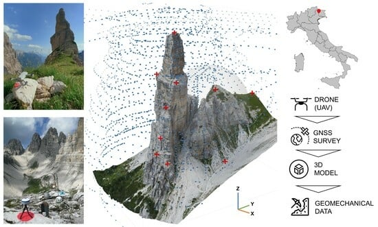
This paper describes a step-by-step procedure employed to build a high-quality, high-resolution 3D model of a rocky pinnacle located in the Dolomites, in northern Italy. The pinnacle, commonly referred to as “Campanile di Val Montanaia” in view of its slender and tower-like shape (loosely translated as “bell tower of the Montanaia Valley”), constitutes a major challenge for topographic and geological surveying due to its high elevation, steep cliffs, and difficulty of approach. The site will represent a natural laboratory for testing a multi-disciplinary approach for the comprehensive topographic, geomechanical, and geophysical characterization of geological objects. The construction of a 3D model represents the first step in such a multi-disciplinary approach, as it will allow for (a) the extraction of rock mass discontinuity data and the assessment of its degree of fracturing, (b) a geomechanical numerical analysis aimed at investigating the stability and deformation mechanisms of the pinnacle, (c) the dynamic characterization of the object through geophysical numerical modeling (which will be presented in a separate paper), and (d) the creation of a baseline for long-term monitoring of deformations and volume loss due to progressive erosion and rockfall detachment.
The quality and quantity of geological data that can be extracted from a 3D SfM model generally depends on its accuracy and detail, which, in turn, are functions of the resolution and ground pixel size of the photographs, and, thus, the distance from which photographs are taken [
14]. At the same time, the construction of denser 3D point clouds and meshes with high or very high resolution comes at the expense of longer processing times and requires high-end workstations that may not be readily available even to the professional user. Understanding the relationship between model detail, resolution (and, thus, quantity and quality of extracted data), and computational effort can assist in the identification of a good compromise between high detail and short processing time. To do so, in this paper we build models with progressively higher quality and detail, which are then employed for rock mass discontinuity mapping (e.g., [
15]).
Ultimately, the objective of the research is the construction of a digital twin [
23] that will allow the physical and mechanical behavior of the pinnacle to be analyzed in future studies, in order to forecast and monitor its behavior and long-term geomorphic evolution and their implications in terms of potential landslide hazard and risk.
2. Overview of the Study Area
The study area is located in the upper Montanaia Valley, within the Cimoliana Valley watershed, 12 km north of the town of Cimolais (province of Pordenone, northeast Italy) (
Figure 1a). The pinnacle is part of the Friulian and Oltre Piave Dolomites system, which, together with the other eight dolomitic systems, has been included in the list of Unesco World Heritage Sites since 2009.
The rocky pinnacle of the “Campanile di Val Montanaia” and the surrounding area are formed by dolostone of the Dolomia Principale formation [
24], which was deposited in a shallow lagoon environment in the Upper Triassic (Norian to Rhaetian, 216–199 million years ago), and is locally characterized by a maximum thickness of about 1500 m [
25] (
Figure 1b). The dolostone is organized in layers of variable thickness, up to a few m, that dip slightly to the southeast (
Figure 1c).
The pinnacle is located at the center of a glacial cirque constituted by sub-vertical rock slopes, the bases of which are covered by active, unvegetated talus deposits. The genesis of the pinnacle is due to the erosive action of the glacier that existed in the area until the end of the last glacial maximum (LGM), about 10,000 years b.p. [
26]. The Campanile has a maximum height of about 240 m, measured along the southern side (i.e., valley side), and reaches an elevation of 2173 m a.s.l. The pinnacle progressively thickens towards the base, as the upper part has a diameter of about 30 m, which increases to 60 m in the central part. The base of the pinnacle has a more irregular shape, more elongated in the north–south direction compared with the east–west direction (about 100 m and 60 m, respectively). A 10 m wide ledge is clearly recognizable approximately 65 m below the peak, caused by the presence of weaker dolomitic limestone layers that are more erodible than the surrounding dolostone [
26].
3. Materials and Methods
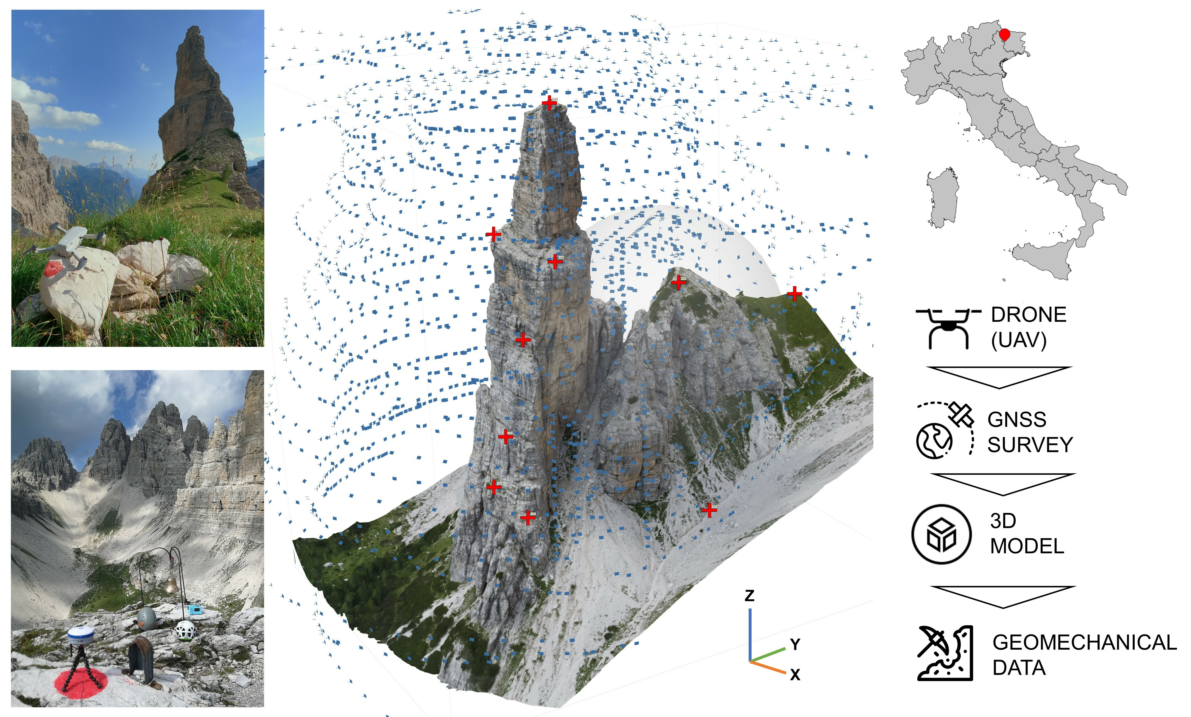
This section aims to provide readers with details about the procedure through which surveys and data processing have been performed, starting from the surveying tools and the field operations, then describing the laboratory part of the work, in terms of photogrammetric modeling and geomechanical analysis (
Figure 2).
3.1. Field and Remote Sensing Equipment
Due to the size, shape, and location of the object to be surveyed, collecting photographs from the ground level was not an option; therefore, a UAV platform was chosen. Approaching the Pinnacle involves about 2 h hiking with an elevation gain of 800 m. Therefore, a lightweight DJI Mini SE (MT2SD25) drone was used instead of a high-end UAV, capable of carrying a full frame camera. The Mini SE is equipped with a 12 Megapixel 1/2.3″ CMOS optical sensor, mounted on a 3-axis gimbal, and a 4.3 mm lens (equivalent to a 24 mm lens in 35 mm format) with a diagonal Field of View (FOV) of 83. The maximum flight time of the drone is estimated to be 30 min in the absence of wind and ideal conditions, while the maximum take-off altitude is 3000 m. Such specific features contributed to the choice of this small but capable drone. A lightweight drone was, in fact, also fundamental to ensure a sufficient autonomy in terms of power supply, which was achieved by carrying six light-weight and small-size batteries instead of the heavy battery packs required for heavy-payload drones. As an additional power source, to maximize the number of flights during the survey day, a simple 20,000 mAh powerbank was used to recharge the batteries that were progressively discharged during flight activities.
To insert the SfM products in an absolute reference system and to increase the geometrical quality of the obtained three-dimensional model, both in terms of scale and shape, temporary GCPs had to be used. To draw the GCP targets without leaving permanent marks, a water washable colored chalk and light cardboard-made mold (about 0.4 m diameter) were prepared (
Figure 3). GCPs were created on the ground surrounding the Pinnacle, along its slopes, and at its peak. To measure the three-dimensional GCP coordinates, GNSS technology was used. In particular, because of the lack of both phone and internet coverage of the area, which would have enabled NRTK [
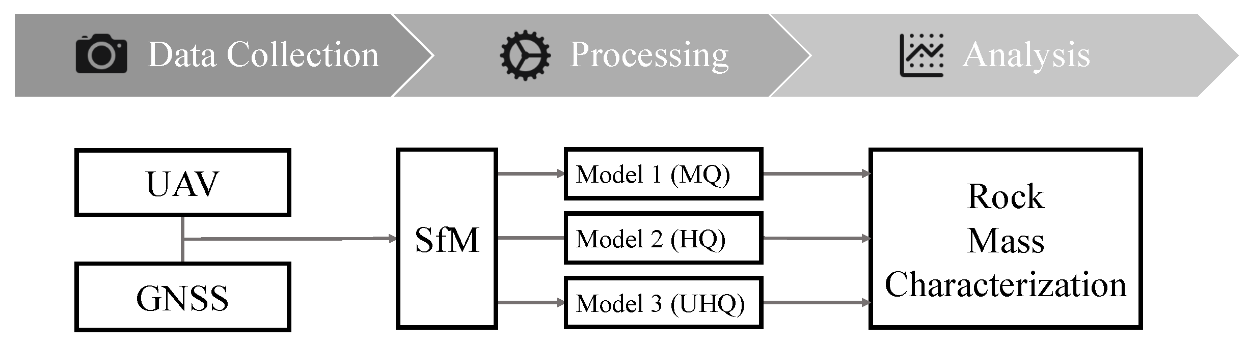
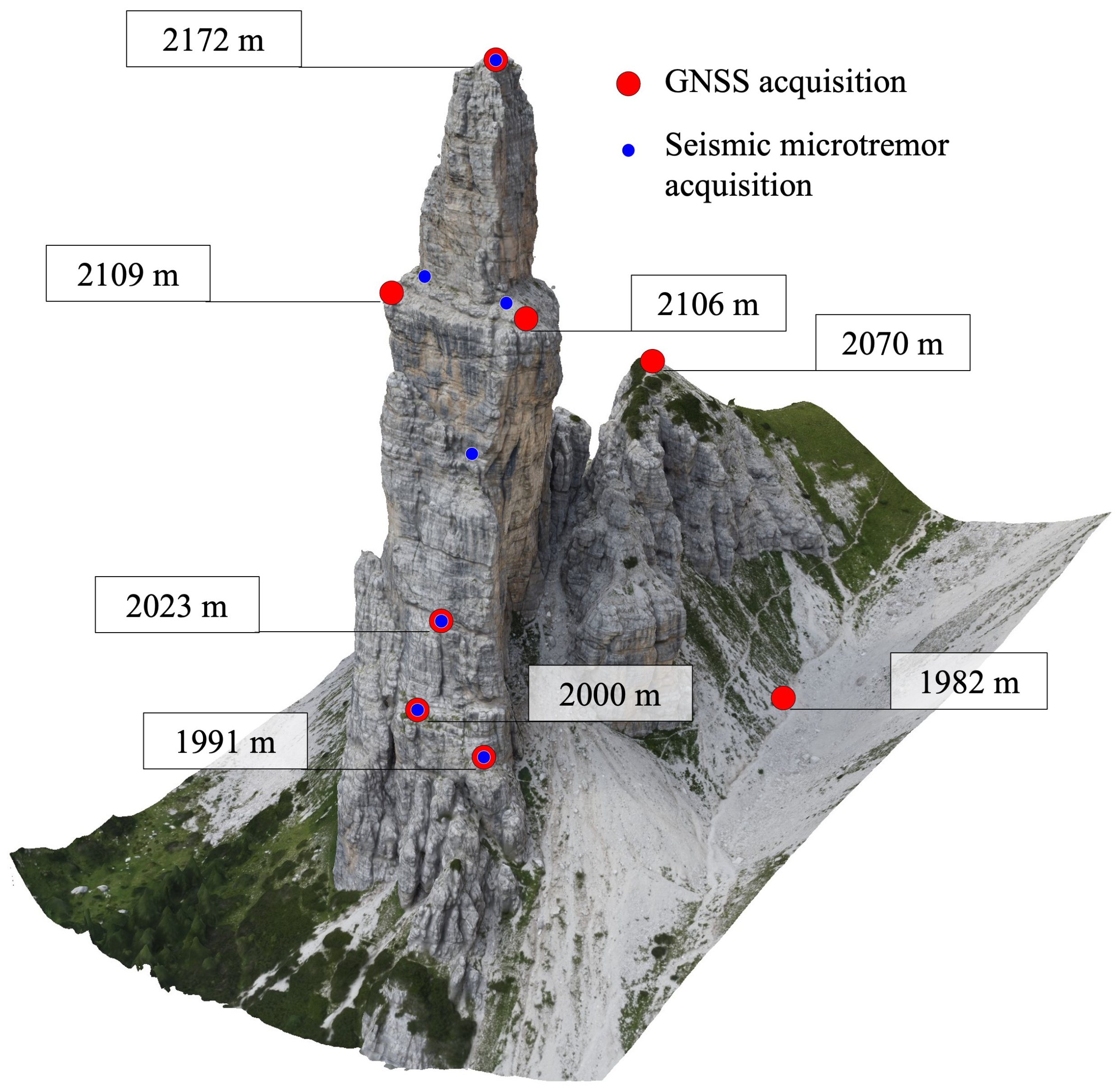
27] precise positioning of a single rover receiver, two GNSS devices (Stonex model S900A) were involved. These are double frequency and full constellation geodetic class receivers. To set the receivers in place, a light photographic tripod and a mini flexible tripod were used, coupled with ad hoc adapters to connect the GNSS antennas. Nine microtremor recordings (16 min each) were also collected by using a portable seismometer (Tromino by MoHo, Italy) at different elevations along the rocky pinnacle. The aim was to experimentally assess the dynamic behavior of the structure (i.e., its natural frequencies and shapes) in order to tune the dynamic numerical modeling of the structure. Microtremor recordings can be used, e.g., to quantify the elastic moduli of the rock and for other dynamical problems that will be dealt with in a separate paper.
3.2. Data Collection Procedure
The surveying operations involved a full day and four people, of which two mainly acted on the Pinnacle and two worked from the base. The climbing team had the main goal of drawing and measuring the GCPs and acquiring the micro-seismic data. One of the two GNSSs was set in place in the open field north of the Pinnacle and acted as a master station, providing the second RTK correction using the classical radio-link approach. The master’s coordinates used for the real-time survey were defined in single point positioning by averaging 3 min of observations. At the same time, the raw phase observables were also acquired by the master station, thus allowing a subsequent refinement of its position by computing in post processing the precise coordinates through the PPP (Precise Point Positioning) approach [
28].
The climb to the top of the “Campanile di Val Montanaia” took about six hours and involved seven main stops corresponding to the GCPs shown in
Figure 4, conveniently placed on ledges as far as possible from the main wall. At each stop, the marker was drawn and then measured through GNSS with 10 min of data acquisition in RTK mode. Furthermore, the rover receiver was set in order to acquire raw phase data along the observing session, in order to allow a post-processing estimation of the baselines with respect to the master. Despite the obstruction of the sky visibility at the wall side of the receiver (mainly north of the rover), thanks to the full constellation capability of the used receiver it was possible to fix the initial phase ambiguities in RTK and work at a few centimeters level of precision. Only in the case of one of the GCPs were the coordinates acquired under “floating” conditions, probably due to both the low number of satellites and the strong multipath caused by the wall next to the rover receiver. Nine microtremor recordings were collected close to each GCP (
Figure 3) to have their precise position on the rock mass. Further, three GCPs were drawn at the base ground around the Pinnacle and measured through the GNSS, following the same procedure used for the others.
To maximize operations during the survey day, a total of 9 flights were conducted with the small UAV. These flights had an average duration of 20 min, including both take-off and landing, resulting in a cumulative flying time of 3 h. This duration was conservatively reduced compared with the maximum range of the drone, which allows for up to 30 min of operations under ideal conditions, taking into account variables possibly impacting the specific working scenario such as the decreased air density at higher altitudes, requiring a greater consumption of energy for flight, the variable winds on the different sides of the pinnacle, and also considering the time for a safe landing.
The drone was flown from the ground base at various intervals during the day in order to have various optimal light conditions and good exposure of the acquired pinnacle side. An attempt was therefore made to take images of the slopes in the shade, following the movement of the sun throughout the day, to mitigate the presence of significant luminous contrast in regions immediately exposed to sunlight. To allow for a better reciprocal positioning between the radio control and the UAV, the drone’s take-off took place from different positions, considering that a flight behind the rocky mass would have immediately caused a loss of signal.
An SRTM-DEM [
29] or InSAR-derived DEM [
30] are usually used to perform automatic flight planning, thus enabling more efficient survey execution. With these raw three-dimensional models, it is usually possible to perform flight planning for the three-dimensional reconstruction of façades, such as in the case of buildings [
31]. However, the “Campanile di Val Montanaia” case study has peculiarities that cannot be captured by the geometric resolution of DEMs obtained from satellites, as it is composed of too complex and irregular sub-vertical shapes. Not having a sufficiently accurate and detailed three-dimensional model of the pinnacle and the surrounding area available in advance, it was not possible to carry out safe automatic flight planning to optimize the trigger points of the images.
Due to the mentioned circumstances as well as considering the logistical difficulties caused by the absence of data connectivity in the surveyed region, the flights were conducted manually with the aim of achieving an optimal distance of approximately 80 m from the observed surface. This distance was chosen to obtain a Ground Sampling Distance (GSD) of approximately 0.03 m.
To improve the efficiency of the flight duration, the drone was operated manually using a sequential method. This involved systematically measuring the vertical overlap between strips of subsequent frames. During each flight, the drone covered a pseudo-circular sector with the camera pointing at the observed slope, while keeping the absolute altitude constant. At the end of each circular sector, the flight elevation varied in accordance with the estimated overlap of 15 m and the following sector was surveyed. In this way, vertical movements that require more flight time, especially with regard to descent movements, were minimized. During the acquisitions, images were also acquired with the camera inclined at 45 to better observe the pinnacle ledges.
It is noteworthy that the GCPs were materialized by the team involved in the ascent to the summit of the pinnacle, a process that spanned a significant portion of the day. As a result, the GCPs were established at the summit during the latter portion of the day. Consequently, any photos captured at the summit prior to the materialization of the GCPs would not have included their location. For this reason, the process of capturing photos started at the bottom of the structure, where GCPs had been set up during the early hours of the day.
3.3. SfM Reconstruction
Various levels of processing were examined during the three-dimensional reconstruction operations using the Structure from Motion (SfM) methodology. These levels of processing had a specific impact on the quality of the dense cloud. It is important to note that the parameters such as input images, GCPs, cleaning operations, and the generation of a unique sparse cloud were kept constant throughout the testing.
As for the GCP coordinates, a post-processing calculation of the baselines between master and rover was performed using the RTKLIB software [
32]. Both RTK and the post-processed solutions were aligned to the ITRF2014 reference frame by computing the master station PPP position by means of the GipsyX software package [
33]. Since the master station acquired raw data for about 8 h, following the results given in [
34], the expected accuracy of the resulting PPP coordinates is at the centimeter level in the plan components and a couple of cm in the height one. The comparison of the final GCP coordinates given by the RTK and the post-processed solutions gives maximum differences of about 2 cm. This confirmed the good quality of the measurements. Additionally, a couple of centimeters of uncertainty should be considered due to the way the GNSS antenna were set up on the GCP targets: visually placed in their center and roughly measuring the vertical antenna height with a tape. Finally, it is reasonable to consider the target relative precision about 3 cm and its global accuracy around 5 cm.
The three-dimensional reconstruction process was carried out with Structure from Motion technique and processed with Agisoft Metashape Professional 2.0.2 (version 16404) software [
35]. Before the processing stage, it was crucial to undertake a careful selection of the pictures that would be used. In this particular study, the manual selection of the frames was considered essential since the flight plan was performed manually. The overall radiometric quality of the photos was found to be satisfactory using analytical detection available inside the software. Photos that exhibited almost full overlap, as well as those with areas of inadequate lighting, were subsequently removed during this phase. A total of 1975 photos were finally selected for processing. Furthermore, the collimation of the GCPs was manually adjusted on the majority of the available photos to improve the overall quality of the model.
The SfM processing was carried out using a workstation with high computing capabilities from the following hardware components: Xeon Gold 6130 at 2.10 GHz CPU, dual NVIDIA GeForce RTX 2080 Ti GPU, and a total of 256 GB of RAM. The initial phase of generating the sparse point cloud required a total of 10 h and 23 min for matching time and another 3 h and 42 min for alignment time. In the initial stage of processing, the sparse cloud was effectively refined through a rigorous examination of point-reproduction errors. The identification of the center of the GCPs in this case study was complicated by some specificities. This was mostly due to the fact that some of the GCPs were captured in photos with a significantly high angle of incidence (
Figure 5). Additionally, during this step, any outliers generated in the cloud and scattered around the main features of the Campanile were manually removed.
After generating the cleaned sparse point cloud, the photogrammetric processing went ahead by computing five different dense clouds with the aim of inspecting the impact of two different parameters: the “reconstruction quality” and the automated “depth filtering” of the outliers. Three solutions were produced at the quality level “high” by setting the filtering level at the values “mild”, “moderate”, “aggressive”. Then, using a “moderate” filtering level, the point clouds with quality “medium” and “ultra-high” were generated too. Differences in the processing times and usability for rock mass analysis were then discussed. Finally, the 3D modeling of the pinnacle was completed, generating the textured colored mesh.
3.4. Geomechanical Analysis
The 3D models were employed to perform systematic digital discontinuity mapping within two distinct windows (i.e., using a window mapping approach, see [
36]). The mapping activity was performed using the free software CloudCompare [
37], which allowed the rock mass discontinuities to be mapped in order to derive orientation (i.e., dip and dip direction) data. The persistence (i.e., the size) of each mapped feature was derived by computing the diameter of the smallest bounding sphere enclosing the feature. The orientations of the mapped discontinuities were then plotted in stereonets (one each for the medium-, high-, and ultra-high-quality 3D models) using the software DIPS [
38]. The average dip and dip direction of the identified discontinuity sets were extracted, and the dispersion of each discontinuity set estimated using the Fisher coefficient “K”. The minimum and maximum size of the identified features were also recorded and compared among the investigated models. The persistence of the smallest mapped features was also extracted.
Based on the results, the advantages and limitations of rock mass discontinuity mapping in higher- vs. lower-resolution 3D models were discussed, also with considerations of the scale of the investigated object, the objectives of the analysis, and the characteristics of the survey.
4. Results
In this section, the main technical results are described. Two main aspects are considered: the quality of the obtained 3D model in relation to the computational effort necessary to produce it, and the usability of the model for discontinuity mapping depending on its quality.
4.1. 3D Model Quality
The present investigation produced diverse outcomes in order to establish an optimal cost–benefit equilibrium in relation to the processing time and achieved results. The primary parameters of the processing are hereafter outlined, considering the considerable variety observed in the complex region surveyed. It should be noted that certain values, such as the GSD, are presented as average values, but have significant variations.
Number of images: 1975;
Average GSD on the rock mass: 0.03 m;
Tie points: 229,111;
Projections: 3,344,884;
Points: 4,501,342 (high-quality dense point cloud);
Reprojection error: 1.69 pixels;
GCP total root-mean-square error (RMSE): 0.06 m.
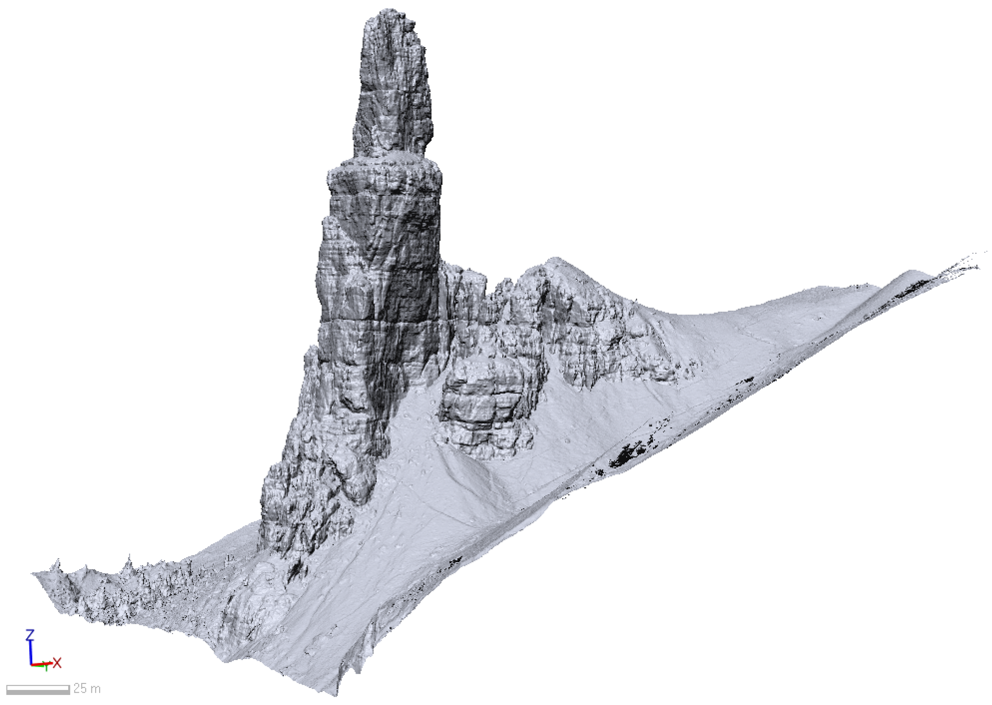
The dense point cloud generation took 2 h and 44 min considering the “medium quality” level, 5 h and 48 min for the “high” quality model, and, finally, 14 h and 35 min using the “ultra-high” quality parameter. The focus on the “depth filtering” mode should be evaluated considering that it is a means of removing noticeable outliers while preserving as much as possible the detailed elements of the three-dimensional model, which are crucial for subsequent analysis. The test demonstrated that, in the case of the Montanaia rock pinnacle, which is characterized by highly irregular shapes, the optimal trade-off between excluding outliers and preserving model complexity falls within the “moderate” filtering level. Moreover, if setting the parameter to “aggressive”, the computational time for such a model increased dramatically. Therefore, all the results discussed in the following are related to dense point clouds computed using a “moderate” depth filtering. An example of the model produced with the SfM processing method is shown in
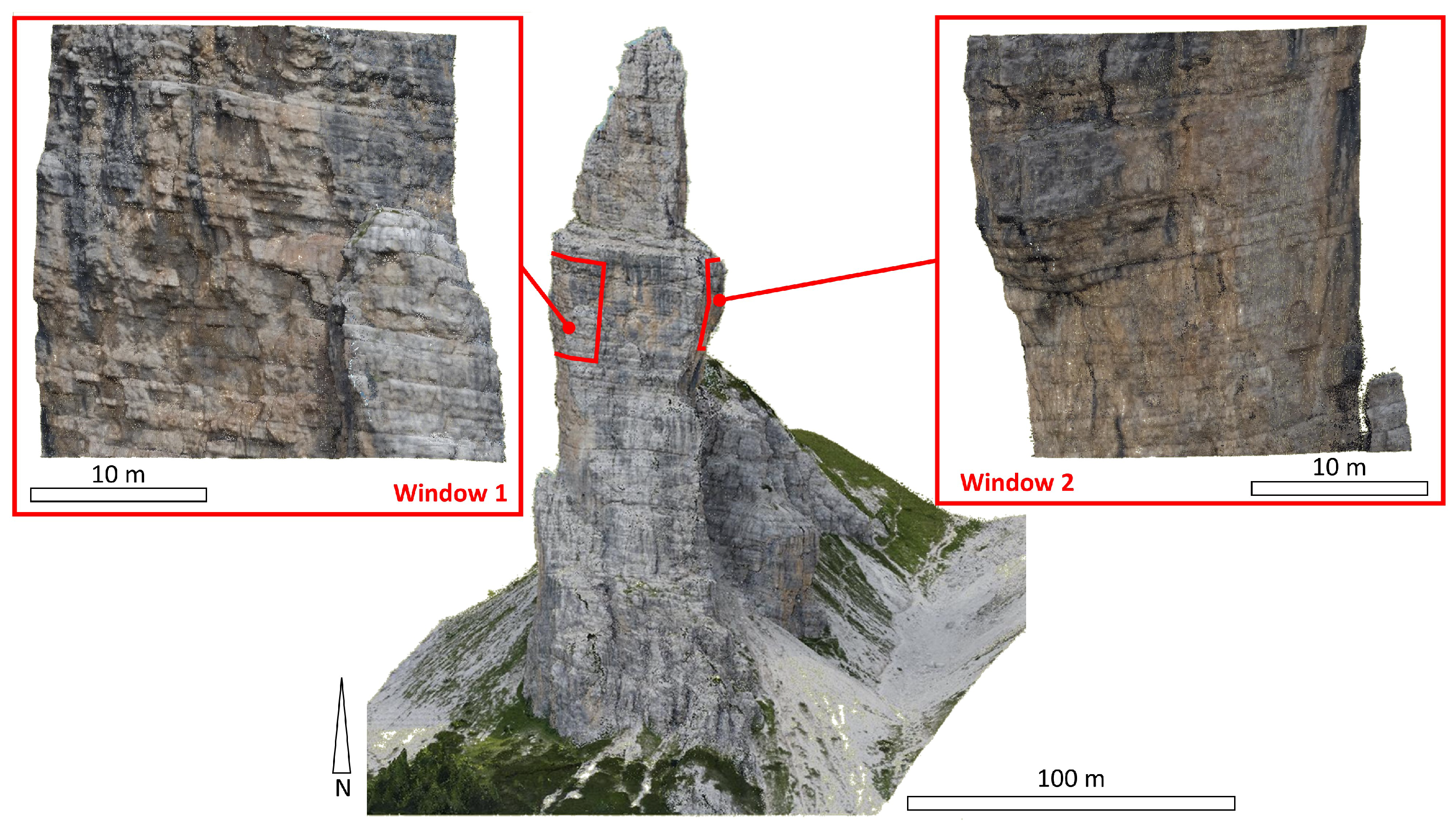
Figure 6, where the mesh, which automatically closed the holes, is depicted. The textured model is reported in
Figure 7, where the specific areas subject to the geo-mechanical analysis are also highlighted.
4.2. Geomechanical Analysis
Two square windows were selected to perform discontinuity mapping on the point clouds derived from the medium-, high-, and ultra-high-quality SfM reconstruction. The discontinuity mapping on the dolomitic rock mass was performed for each window and model quality, and allowed a total of six different datasets to be obtained.
The windows are located on opposite sides of the Campanile (
Figure 7). Window 1 (W1) is located on the western side of the pinnacle and includes its south-western corner. Window 2 (W2) is located on the eastern side and includes the north-eastern corner of the pinnacle. The inclusion of a corner within each window was deliberate and intended to exploit the three-dimensional configuration of the object to provide (a) an improved geometrical constraint in deriving discontinuity orientation data and (b) to limit the orientation bias that typically affects discontinuity mapping performed on outcrops characterized by a single orientation. The square windows W1 and W2 are characterized by a 35 m and a 32 m side, respectively. The point counts for W1 are 131,202 for the medium-quality model, 593.084 for the high-quality model, and 3,259,078 for the ultra-high-quality model. The point counts of W2 are 93,736 for the medium-quality model, 400,181 for the high-quality model, and 1,924,666 for the ultra-high-quality model.
Table 1 summarizes the results of the discontinuity mapping performed on each window. In most cases, four discontinuity sets were observed. The most represented set is the stratification of the dolostone deposit (D1), which dips with a low angle (typically, less than 10°) in an eastern to south-eastern direction. The other sets (D2–D4) are constituted by high angle, sub-vertical discontinuities that strike in a north–east, north, and north–west direction, respectively, (
Figure 8). The Fisher’s K value [
38], which is a value that describes the dispersion or tightness of a cluster of points, is also reported for each set. A smaller K value indicates a greater dispersion of the set, whereas a greater K value indicates a tighter cluster.
Figure 9 and
Figure 10 show the stereonets derived from the discontinuity mapping for windows 1 and 2, respectively. For each model, two stereonets are presented, displaying the concentration of poles of the bedding planes and the sub-vertical discontinuity sets. This solution prevents the contouring of pole density to become saturated near the center, due to the pole cluster of bedding planes, which would pose challenges in the identification of the other sets. The number of discontinuities mapped in the models appears to increase with the quality of the reconstruction and the density of the point cloud. However, in window 2, a decrease in mapped discontinuities was observed, due to the increase in noise within the point cloud that locally limited the visibility of bedding and vertical discontinuity planes and traces (
Figure 7).
Intuitively, the smallest feature mapped in each survey was also found to be strictly correlated with the quality and density of the investigated point clouds. For window 1, the smallest mapped features for the medium-, high-, and ultra-high-quality models were 6 m, 1.7 m, and 0.7 m, respectively. For window 2, the smallest mapped features were 1.8 m, 1.1 m, and 1.3 m. The increase in the persistence of the smallest mapped feature in the ultra-high-quality model of window 2 is probably related to the already mentioned increase in the noise and frequency of outliers across the point cloud.
The orientation of the observed discontinuity sets displays a good correlation with discontinuities and structural features at the scale of the entire pinnacle.
Figure 11 shows a nadiral orthophoto of the area of the pinnacle, retrieved from the Friuli Venezia Giulia air photo repository (
https://eaglefvg.regione.fvg.it, accessed on 10 July 2023), on which the traces of sub-vertical structural lineaments have been outlined. Two major lineament trends (L1 and L2) can be observed striking in approximately a NW–SE direction, which can be correlated with discontinuity set D2. A third, minor lineament trend, striking in a NE–SW direction, can also be observed, which correlates with discontinuity set D4. The agreement between the orientation of the lineament and the sub-vertical discontinuities (except for discontinuity set D3, which does not display clear correlations with any lineament trend) emphasizes the role of structural geology in controlling the morphology of the Campanile, and possibly its long-term evolution and stability.
5. Discussion
The particular shape, dimension, and location of the surveyed rock pinnacle contribute to diverse multidisciplinary investigations. Additionally, the substantial amount of collected data holds potential for extensive analysis that exceeds the goals of this study. In this section, we discuss the limitations of this work and possible further developments.
From the photogrammetric point of view, a crucial aspect in the process of capturing imagery for the survey of a complex object, as the one examined in this study is, relates to the possibility of implementing an analytical flight plan specifically designed for UAVs. To achieve an efficient and safe flight in a complex area, it is necessary to establish a primitive three-dimensional starting model. This model would serve as a foundation for properly determining the capturing locations of the images. An attempt to build a rough model to better plan the survey was made by using crowdsourced images [
39]. Indeed, it was possible to find some videos online that are accessible to the general public, from which a number of frames were extracted, and a three-dimensional model was produced using expeditious SfM methods. Unfortunately, images acquired from non-professional UAV flights only allows for the creation of an approximate and incomplete model [
40,
41], as there is in fact no way of georeferencing and properly scaling the obtained point cloud. Moreover, having enough crowdsourced data to have a sufficiently complete three-dimensional model is not obvious in general [
42], and that was confirmed in the analyzed case. The results of this expeditious analysis were actually useful to better organize survey operations, but were not sufficiently comprehensive and detailed to safely plan a fully automated UAV flight.
Furthermore, for these reasons, we decided to share the 3D model of the “Campanile di Val Montanaia” according to the principles of Open Science and Open Data, including the final mesh and texture, in a publicly accessible repository (
https://amsacta.unibo.it/id/eprint/7377/, accessed on 1 October 2023). Thanks to this model, it will be possible to carry out rigorous planning of future UAV flights, thus enabling more efficient surveying [
31] and for monitoring purposes. Among the benefits of this type of disclosure, it will be possible to make comparisons and benchmarks in an area that is otherwise complex for logistical issues. Further possible application of the digital twin that accurately represents the “Campanile di Val Montanaia” and its surrounding environs is to transfer the model into a virtual reality environment, enabling users to engage in an immersive visit to the surveyed location. Future developments of this work would include a new UAV survey mission carried out with different sensors and rigorous analytical flight planning. It would also be interesting to evaluate the impact of different configurations and quantities of GCPs on the quality of the final model, its accurate scaling, and the georeferencing. In particular, this case study might be a probing test for UAV direct georeferencing techniques [
43,
44,
45,
46], which in this context would avoid the need of climbing up the pinnacle to set GCPs, thus allowing for a considerably simpler surveying procedure.
The geometrical model obtained in the described way will be used to generate a dynamic numerical model of the pinnacle. The mechanical parameters (elastic moduli) of such a model will be tuned to fit the modal frequencies and shapes determined experimentally by means of the microtremor surveys performed at nine calibration points along the pinnacle itself. This procedure, its results, and their meaning is described in a separate paper in preparation.
Discussing now the geo-mechanical aspects, the characterization of rock masses using three-dimensional models (i.e., point clouds) allows for some of the challenges related to traditional field work to be avoided or mitigated (e.g., rockfall activity, limited site accessibility), and has therefore become a routine activity in engineering practice. Over the past decade, the introduction of SfM photogrammetry provided significant benefits and contributed to the development of cost-effective workflow and applications for rock mass characterization, and particularly for discontinuity mapping. Its ease-of-use, particularly compared with traditional digital photogrammetric methods [
6], allowed professionals and geoscientists to rapidly become familiar with digital photogrammetry engineering applications. In this paper, we investigated the advantages, limitations, and challenges of performing discontinuity mapping using medium-, high-, and ultra-high-quality models. We noted that, intuitively, higher-quality models (i.e., characterized by higher point density) allow for a more detailed mapping of discontinuity traces and planes. Smaller discontinuities, characterized by low persistence values, can generally be identified in denser models. The selection of points that, within the model, form traces of discontinuities is also easier and generally more precise, allowing for a more accurate estimation of both orientation (i.e., dip and dip direction) and trace length. However, together with the increased density of the point cloud, an increase in noise was observed, with a higher number of outliers that locally made the identification of discontinuities, and the selection of points for interpolation, significantly more challenging. The amount of noise in the model may change based on the multiple survey parameters, including flight distance from the object, the ground pixel size, quality of the sensor, and lighting conditions, which can cause the brightness across the scene to vary both spatially (due to the roughness of the object) and temporally (due to the change in the relative position of the sun during the survey). In light of these considerations, but also bearing in mind the computational cost necessary to build the different models shown in the previous section, the most convenient Metashape parameter combination is the use of a “high” reconstruction quality and a “moderate” depth filtering. This parametrization was also used to build the model that is now publicly available.
Indeed, the number of outliers within higher density models may be limited through post-processing, filtering, and cleaning of the point cloud. However, as the number of points exponentially increases with model quality, the filtering and cleaning process, particularly when undertaken manually, may be significantly time consuming and computationally expensive. In the presented analysis, we decided not to perform additional the post-processing and filtering, besides those automatically or semi-automatically performed on the sparse point cloud within Metashape, to avoid introducing subjectivity into the process. In fact, a certain degree of subjectivity was introduced during the discontinuity mapping process. This is, however, inevitable, as evidenced by studies that compare the differences in the interpretation of geological datasets provided by professionals and academics with varied degrees of experience and seniority (e.g., [
47]). In this study, we attempted to mitigate the subjectivity by limiting the number and size of the mapping windows, and by assigning the discontinuity mapping task to a single, experienced individual.
We emphasize that the size of the window, and the cut-off size of the smallest features that are mapped, is strongly dependent on the objective of the rock mass characterization and the scale of the investigated problem. In general, the characterization of small, dm-scale discontinuities can be performed to investigate local variations in rock mass quality and behavior, and to create highly detailed discrete fracture networks (DFNs) for advanced numerical modeling analysis [
48]. In such cases, very high-resolution models should be employed, and the survey should be planned in order to optimize quality (e.g., using very high-resolution sensors or reducing the survey distance). However, rock mass characterization aimed at the analysis of the stability at the slope scale seldom requires the mapping of cm- or dm-scale structural features. In fact, m- or Dm-scale discontinuities are significantly more capable of providing kinematic release for larger volumes, compared with smaller discontinuities, and therefore they are more effective in controlling the stability, behavior, and evolution of rock slopes.
6. Conclusions
This research paper outlines the process of creating a high-quality and detailed three-dimensional model of a rocky pinnacle located in the Dolomites region through the utilization of SfM methodology. In particular, a specific workflow for data collection, processing, and geomechanical analysis was optimized and tested on a challenging object such as the “Campanile di Val Montanaia”, producing its digital twin. The survey activities also considered micro-seismic acquisitions, not discussed in this paper, that will be analyzed by coupling them with the geometrical description of the rock mass. This case study constitutes a highly multidisciplinary work, both in the field surveying operations and in the data analysis. It showcases the inherent capabilities of 3D models in the mapping of rock mass discontinuities, shedding light on the complex relationship between model quality, resolution, and computing effort. The findings emphasize the significance of reaching a balance between the level of detail and the time required for processing in order to achieve an optimal equilibrium between costs and benefits. We examined the constraints and difficulties associated with utilizing 3D models for the purpose of discontinuity mapping, which encompasses the introduction of subjectivity during the interpretation of geological evidence. Potential future work includes taking advantage of new sensors and enhanced analytical flight planning techniques for conducting further UAV surveys, such as higher-resolution optical sensors, LiDAR (e.g., for change detection analysis), and thermal cameras (e.g., for groundwater seepage analysis).
In addition, the 3D model of the “Campanile di Val Montanaia” has been made openly available, creating the opportunity for several further applications, such as converting the current model into a virtual reality environment. This model can also be used as a baseline for the geometrical monitoring of the rocky pinnacle through repetitions of the survey over time, for overall structural movement, or potential rockfall detachment. The natural frequencies of vibration measured on the pinnacle will also be the basis to calibrate dynamic numerical models of the structure as well as to monitor possible variations in the geometry or in the mechanical properties of the rocky formation over time. Overall, this study contributes to our understanding of the behavior and evolution of rock slopes and offers significant new knowledge for challenging surveys and their applications.

 ,
, 


