Article

Mapping Grassland Based on Bio-Climate Probability and Intra-Annual Time-Series Abundance Data of Vegetation Habitats

1
College of Land Science and Technology, China Agricultural University, Beijing 100193, China
2
Key Laboratory of Remote Sensing for Agri-Hazards, Ministry of Agriculture, Beijing 100083, China
*
Author to whom correspondence should be addressed.
These authors contributed equally to this work.
Remote Sens. 2023, 15(19), 4723; https://doi.org/10.3390/rs15194723
Submission received: 30 August 2023 / Revised: 19 September 2023 / Accepted: 23 September 2023 / Published: 27 September 2023

Abstract

:
Accurate inventories of grasslands are important for studies of greenhouse gas (GHG) dynamics, as grasslands store about one-third of the global terrestrial carbon stocks. This paper develops a framework for large-area grassland mapping based on the probability of grassland occurrence and the interactive pathways of fractional vegetation and soil-related endmember nexuses. In this study, grassland occurrence probability maps were produced based on data on bio-climate factors obtained from MODIS/Terra Land Surface Temperature (MOD11A2), MODIS/Terra Vegetation Indices (MOD13A3), and Tropical Rainfall Measuring Mission (TRMM 3B43) using the random forests (RF) method. Time series of 8-day fractional vegetation-related endmembers (green vegetation, non-photosynthetic vegetation, sand land, saline land, and dark surfaces) were generated using linear spectral mixture analysis (LSMA) based on MODIS/Terra Surface Reflectance data (MOD09A1). Time-series endmember fraction maps and grassland occurrence probabilities were employed to map grassland distribution using an RF model. This approach improved the accuracy by 5% compared to using endmember fractions alone. Additionally, based on the grassland occurrence probability maps, we identified extensive ecologically sensitive regions, encompassing 1.54 (104 km2) of desert-to-steppe (D-S) and 2.34 (104 km2) of steppe-to-meadow (S-M) transition regions. Among these, the D-S area is located near the threshold of 310 mm/yr in precipitation, an annual temperature of 10.16 °C, and a surface comprehensive drought index (TVPDI) of 0.59. The S-M area is situated close to the line of 437 mm/yr in precipitation, an annual temperature of 5.49 °C, and a TVPDI of 0.83.

1. Introduction

Climate change has become a global concern due to the enormous greenhouse gas (GHG) emissions that trigger extreme weather events and pose a threat to terrestrial ecosystems [1,2]. Thus, numerous mitigation strategies have been proposed to mitigate GHG emissions. A total of 127 countries have already announced their carbon emission reduction timetables [3]. As the largest emitter, China has set its goals for carbon peak and carbon neutralization by 2030 and 2060, respectively. Grasslands play an important role in carbon mitigation, storing about 34% of global terrestrial carbon. Additionally, nearly 3.4 billion livestock are responsible for about 7.1 billion tons of carbon emissions per year [4,5,6,7]. Grasslands cover a total of 3.92 million km2 in China, accounting for about 12% of global grasslands [8]. Nevertheless, socioeconomic changes and extreme climatic events have led to substantial changes in grasslands, degrading their structures and functions [9,10]. These dynamic changes in grassland vegetation constitute one important constraint for estimating grassland carbon sequestration. Thus, it is of high importance to explore precise and comprehensive dynamic inventories of the complete carbon budget for grasslands in China.
In spite of some land-cover products, including grassland [11], they only provide rough divisions of grassland types, which hardly meet the demands of decision makers. Different departments have their unique demands of grassland classification units and accuracy. Consequently, this presents challenges for producing accurate maps of grassland types quickly and efficiently. Thus, high standards of methodology in grassland investigation not only can address different demands of decision makers but also can ensure information transfer between product levels to avoid duplication of effort and inconsistent results.
Traditional methods (e.g., hand-drawn mapping through field work and use of satellite maps) are time- and resource-consuming. Satellite data can provide routine coverage over large and remote areas, making the use of such data a cost-effective means of replacing or complementing field data collection in grassland mapping [12]. Effective grassland mapping should consider various factors of grassland evolution and needs to be applicable across different bioclimate zones. However, recent studies have mostly focused on measurable biophysical characteristics for grassland mapping instead of from an ecological standpoint [13,14,15]. Based on bio-climate indicators, it is critical to recognize the ecological traits of different grassland types when mapping grasslands. Many researchers identified bio-climate zones based on meteorological station data [16,17] and obtained patch-like distribution maps, but they ignored detailed variations in grassland communities due to their hidden terrains. Satellite-based meteorological and geographical data can provide continuous information from space and present the habitat states of complex bio-climate environments [18,19]. Additionally, different spatial–temporal–spectral satellite products can improve the understanding of the interaction of multi-level habitat information, which can facilitate the top-down transmission and bottom-up aggregation of knowledge on grassland ecosystems [20].
The high variabilities of grassland bio-climate characteristics make grassland mapping more difficult, and their often overlapping boundaries mean it is challenging to make crisp decisions [21]. Thus, it is necessary to consider the attribute possibility of the characteristics under investigation, indicating within-class heterogeneity. Fuzzy classification models, like random forests (RF), Gaussian process model (GPM), support vector machines (SVMs), and logistic regression (LR), can be used to extract the probabilities of occurrence of different grassland types based on bio-climate factors [22,23,24,25,26].
In addition to macro-indicators of bio-climate characteristics, the evolution of grassland is also regulated by soil and habitat status. By considering four or five generic endmembers (such as soils and substrates, green vegetation, and dark surfaces (abbreviated as SVD), along with local saline land and non-photosynthetic vegetation), the standard spectral endmember space (SVD space) can use a linear spectral mixture analysis model (LSMA) to effectively reveal the interactive process between vegetation and habitats [27]. Moreover, the abundance characteristics of spectral endmembers are also more stable for land surface mapping compared to spectral reflection values [28]. The SVD space has been adopted in the application of multi-scale remote sensing interpretation frameworks of grassland systems [29,30,31].
Due to grasslands’ distinct plant phenology and management (e.g., grazing and mowing activities), it could be more effective to use multi-temporal series images than images obtained using single date acquisition [27,32]. However, it is difficult to confirm a stable and unified typical multi-phase of grassland phenology in large regions due to complex human activities. Thus, dense time-series images are highly valued. In a temperate dryland grass system, a fixed set of four broad endmembers (i.e., green vegetation (GV), sand land (SL), saline land (SA), non-photosynthetic vegetation (NPV), and dark surfaces (DA)) has been validated using multi-seasonal TM images, time-series GF-1 images, and time-series MODIS images [27,33,34].
Therefore, taking Inner Mongolia as the study area, this study develops a novel framework for grassland mapping in a large area based on remote sensing bio-climate characteristics and information on the interactions of vegetation and habitats from time series of endmembers. The specific objectives are as follows: right (1) propose a quantification strategy of grassland bio-climate factors using the RF model for establishing the probabilities of occurrence of grassland types and for partitioning different grassland bio-climate zones; (2) construct the SVD space of 8-day intra-annual MOD09A1 images for mapping different grassland distribution; and (3) analyze the resilience and critical transitions of potential grassland types, as well as the characteristics of grassland evolution in Inner Mongolia over the last 40 years.

2. Materials and Methods

2.1. Study Area

The total area of Inner Mongolia is 118.3 × 10⁴ km2 (Figure 1), which provides the largest livestock products in China. Inner Mongolia has different climate zones, including temperate continental monsoon, cold temperate continental monsoon, and temperate continental climate types. Its annual precipitation is around 377 mm and decreases from east (825 mm) to west (11 mm); additionally, its average annual temperature is around 6 °C. The terrain is mainly characterized by plateaus, with an average elevation of 1000 m, as well as some plains and mountains located in the eastern region. Grassland is the predominant land cover, accounting for more than 70% of the area, and including temperate steppe type (TST), temperate meadow steppe type (TMST), lowland meadow type (LMT), montane meadow type (MMT), temperate desert steppe type (TDST), temperate steppification desert type (TSDT), and temperate desert type (TDT). These grassland types consist of, but are not limited to, typical grasses, such as Leymus chinensis, Stipa baicalensis, and Cleistogenes squarrosa in meadow; Stipa grandis and Artemisia frigida in steppe; and Haloxylon ammondendron and Nitraria tangutorum Bobr. in desert. The diverse ecological climate and grassland types in Inner Mongolia make it highly suitable for developing and testing a novel framework for large-area grassland mapping.

2.2. Data Sources

2.2.1. Satellite Data

The satellite data mainly include Moderate Resolution Imaging Spectrometer (MODIS) data, Landsat data, TRMM data, and STRM DEM data; the detailed information is presented in Table 1.
The MODIS data include land surface reflectance products (MOD09A1), temperature products (MOD11A2), and vegetation products (MOD13A3), covering the study area with 8 scene imageries numbered h25v03, h25v04, h25v05, h26v03, h26v04, h26v05, h27v04, and h27v05. The MOD09A1 products can provide the highest-quality observation of daily surface spectral reflectance from band 1 to band 7, using the best representative pixel of an 8-day retrieval period and a 500 m sinusoidal projection. The MOD11A2 products are provided with the best representative pixel of an 8-day retrieval period and a 1 km spatial resolution, while the MOD13A3 products are the products of monthly synthesis with a 1 km spatial resolution.
The TRMM 3B43 V7 products recorded hourly precipitation (mm/h) from 2001 to 2019. These multi-satellite precipitation data have been widely applied in meteorological analysis [35,36]. Thus, we first created monthly versions of the data by aggregating 24 h of daily precipitation and summing the values for each day of the corresponding month, and then downscaled the resolution of the TRMM data from 0.25° × 0.25° to 1 km, using a multivariate linear regression model based on the MOD11A2 and MOD13A3 products for spatial resolution matching [19,37].

2.2.2. Field Sampling

After interviews with investigators from the China Land Surveying and Planning Institute, we learned that the national grassland special survey (NGSS) samples for grassland mapping were field sampled from July to September in 2019 and 2020. This dataset was initially designed to support national land resource surveys and management in being highly credible. The layout method of NGSS was a combination of stratified sampling and simple random sampling. Each site was selected in a patch that was larger than 1000 m2 with an a priori homogeneous plant community. In total, there are 918 effective sample plots (Figure 1), with records of their locations, altitudes, grassland types, vegetation coverages, biological fresh weight, and dry weight.
Except for the 918 sample plots of grassland, we also effectively collected 627 sample plots from other land types based on Google Earth, including 284 cultivated land samples, 106 forest land samples, 103 bare land (bare soil and desert) samples, 44 water area samples, and 90 construction land samples. The number of sample points of different land types was proportional to their coverage area in our study area. These land-use/cover sites were judged empirically based on the varying satellite image characteristics of different land types. For instance, arable land typically displays clear and regular boundaries, while forests often exhibit high coverage and cast dark shadows. We note that we intentionally avoided referring to any classification maps during the labeling process to prevent subjective bias from influencing our training process [38,39,40].

2.3. Methods

The mapping framework in this study was based on the bio-climate environment and information on the interactions of vegetation and habitats from the time series of endmembers (Figure 2). Firstly, grassland bio-climate factors were constructed based on satellite-based data, and the RF method was used to predict grassland occurrence probability and divide the bio-climate regions. Then, intra-annual standard spectral endmember spaces were constructed based on the MOD09A1 products. Finally, maps of grassland types were created using the grassland occurrence probability and intra-annual spectral endmember spaces with the help of the RF model.

2.3.1. Grassland Type Classification System

The China Grassland Type Classification System (CGTCS) was developed by the “Animal Husbandry Bureau of Ministry of Agriculture” (http://www.xmsyj.moa.gov.cn, accessed on 18 September 2023), dividing grasslands in China into zonal grasslands and intra-zonal grasslands (Figure 3). Four temperature gradient levels were used to divide grassland types in China, including tropical, warm, temperate, and alpine. Regarding surface moisture, grasslands in China were further divided into four gradient humid levels, namely desert, steppification desert, desert steppe, steppe, and meadow. Overall, the CGTCS comprises 14 categories of zonal grasslands, which exhibit typical zonal characteristics. Additionally, it encompasses 4 types of intra-zonal grasslands, primarily affected by local terrain and surface moisture characteristics. Figure 3 provides a detailed overview of the CGTCS. According to this classification system, there are seven types of grassland in Inner Mongolia, namely TDT, TSDT, TDST, TST, TMST, LMT, and MMT.

2.3.2. Grassland Bio-Climate Factors and Probability

The growth of grassland was affected by the local bio-climate environment, including land surface temperature, moisture, and topographic and hydrological conditions. This study constructed grassland bio-climate factors based on satellite-based data. The specific quantitative schemes of grassland bio-climate factors are shown in Table 2.
Based on the habits of herbage cultivation, temperature plays a crucial role in determining growth patterns during the warm season, as well as the total photo temperature and the length of the growth period. A daily average temperature of 0 °C is critical for both the beginning and the end growth of most grasslands. An accumulated temperature of >0 °C indicates the thermal conditions of grassland plants in the growth period. Otherwise, the average temperatures of the warmest month and the coldest month can also be used with the accumulated temperature of >0 °C to better construct the index gradient and generate the bio-climate boundary threshold. These photo-temperature indices were obtained through the MOD11A2.
Another influencing factor is land surface moisture, which is regulated by precipitation, evaporation, and other biological factors. Therefore, the surface comprehensive drought index (TVPDI) was used to reflect land surface moisture, which was derived from the Euclidean distance calculated using TRMM 3B43, MOD11A2, and MOD13A3. For a detailed introduction to TVPDI, see [41].
Non-zonal grassland types were developed under the influence of complex and local topographic conditions. These areas tend to have high groundwater levels and soil water contents, and this humid environment promotes the occurrence of swamp and meadow types. These types of grassland bio-climate conditions could be identified through a comprehensive analysis based on STRM DEM and TVPDI.
Grassland bio-climate factors are natural indicators of vegetation succession [42]. The fluctuation and complexity of climate and habitat state mean that the direction of vegetation succession varies. It was assumed that each type of grassland has its own probability of occurrence in the same plot, and the grassland type with the greatest probability could represent the natural succession direction. The grassland occurrence probabilities were generated using the Random Forest Classifier model with the “predict-proba” from the scikit-learn library available in the Python programming language. The predicted grassland occurrence probabilities of the input samples were computed as the mean predicted class probabilities of the trees in a forest, and the probability of a single tree was the fraction of the samples of the same class in a leaf. According to the type of grassland vegetation in our study area, we ultimately obtained 7 distribution maps of grassland occurrence probabilities. The grassland type with the maximum probability reflects the stable eco-climatic states as the bio-climate zones of the corresponding grassland type. Furthermore, we conducted an analysis of the trade-offs between various grassland types using occurrence probability values. In cases where the occurrence probability difference between two grassland types was less than 10% within the same grid, it signified critical transition areas, suggesting potential shifts in succession dynamics.

2.3.3. Surface Spectral Endmember Space

The linear spectral mixture analysis (LSMA) model assumed that the spectral curve of the mixed pixel was linearly composed of the spectral curve of the pure endmember in each pixel. The purpose of spectral unmixing was to determine the abundance of each endmember in the mixed pixel. The process of time-series LSMA has three steps, including determining the representative seasonal phases of the endmembers, extracting the endmember spectral curves, and unmixing the endmember abundance map with these endmember spectral curves. A detailed description of the LSMA method and endmember selection can be found in Sun et al. [43], and our study used principal component analysis (PCA) to determine the phases [44,45]. This study identified five endmembers, namely GV, SL, SA, NPV, and DA, to illustrate the characteristics of vegetation and habitat in Inner Mongolia. Additionally, the unmixed results were estimates using root mean squared error (RMSE).

2.3.4. Grassland Mapping in Inner Mongolia

The high-frequency time series of endmember abundance data provides rich information about surface cover change but also significantly reduces the operation efficiency. Additionally, the abundance maps of different time phases and different endmembers are inter-coupling and have strong correlations, which also decrease the effects of modeling accuracy [46]. Thus, feature reduction is important to address the large numbers of input features. PCA was used once again to reduce the dimension of the time-series endmember abundance maps and obtain the uncorrelated characteristic parameters.
After obtaining the modeling variables from the compressed time series of endmember abundance maps using PCA, we used the RF model for classification. RF is an advanced ensemble learning method that combines multiple classification and regression trees (CART) to improve accuracy [47,48]. RF is capable of handling high-dimensional datasets, accepting various measurement scales for both numeric and categorical variables. Additionally, it exhibits lower sensitivity to noise, accommodates numerous input variables, and avoids overfitting [49]. The algorithm randomly selects a subset of samples (2/3 of data samples) for the training of each individual decision tree, with the remaining samples (1/3 of data samples) being assigned as out-of-bag (oob) samples that are used to test the classification and estimate the error. For each individual tree, the Gini index (a measure of class homogeneity) is used to perform the best split of a random set of input features at each node. Using a majority vote, a final class is assigned from the multiple outputs of all constructed decision trees. The RF classifier requires only two input parameters, namely the number of trees (N) and the number of variables, to split at each node (m). In this study, N was set to 500 and m = 5. Grassland occurrence probability maps and top 90% cumulative contribution principal components (PCs) were input into the RF model and used for training the model on classifying the sample sites.
To evaluate the effectiveness of occurrence probability in the classification process, we conducted control tests using two configurations: one incorporating the initial 90% cumulative contribution PCs along with 7 occurrence probability maps (trial 1) and another utilizing only the initial 90% cumulative contribution PCs (trial 2). Finally, we evaluated the accuracy of these results using validation metrics based on the confusion matrix, including overall accuracy (OA) and the Kappa coefficient (Formulas (1) and (2)). Moreover, we also provide the basis for estimating the area of classes with the error matrix or transition matrix [50].
OA = 1 N i = 1 r x i i
Kappa = N i = 1 r x i i i = 1 r ( x i + × x + i ) N 2 i = 1 r ( x i + × x + i )
While the N represents the total number of samples, x i i denotes the count of samples correctly identified for land cover, and r indicates the number of land cover types.

3. Results

3.1. Grassland Bio-Climate Probability Maps and Grassland Bio-Climate Zoning

The grassland bio-climate probability maps are illustrated in Figure 4b–h, representing the preferred habit location of various grassland types. The largest probability was used to generate the bio-climate zones, which considered the theoretical territory of each grassland (Figure 4a). Potential types of grasslands included TDT, TSDT, and TDST, covering a total of 418 × 103 km2, or about 36% of our study area, and they are mainly located in the west of Inner Mongolia. The typical temperate bio-climate zones (46%) of TST and TMST were predominately distributed in the middle of Inner Mongolia, and their area amounted to 486 × 103 km2 and 61 × 103 km2, respectively. The intra-zonal bio-climate types were mainly located in the mountains and valleys of eastern Inner Mongolia, covering 18% of the total area, and the grassland types of LMT and MMT covered a total area of 61 × 103 km2 and 157 × 103 km2, respectively.

3.2. The critical Transition Zones of Latent Succession of Typical Grassland Types

Desert, steppe, and meadow represented alternative stable grassland states in Inner Mongolia, implying that the critical transitions of grassland types would be in response to bio-climate changes. Bio-climate zones and grassland occurrence probabilities explained the natural driving force of each grassland type, and ecotone indicated the natural vulnerability and resilience between different stable grassland systems. Critical transition areas were extracted where the difference in occurrence probability of two grassland types was less than 10% in the same grid (Figure 5). It is evident that the west–central part of the study area, which is located at the 310 mm precipitation line and has an annual average temperature of 10.16 °C and a TVPDI of 0.59, has a critically sensitive transitional zone of 1.54 × 10⁴ km2 of desert-to-steppe (D-S) transition region that requires careful policy guidance. For instance, protective measures such as prohibiting grazing can be implemented to prevent the degradation of 8600 km2 of grassland in this region. Additionally, a scientifically based recovery program, which includes activities like planting native grass species and implementing water conservation techniques, can be established to restore 6800 km2 of the desert. The steppe-to-meadow (S-M) region overlaps with the northern pastoral ecotone, with an area of 2.34 × 10⁴ km2. This area has favorable hydrothermal conditions that facilitate competition not only with the TST-TMST but also with other lands (like arable land and woodland). It is mainly round, with an annual average precipitation of 437 mm, an annual average temperature of 5.49 °C, and a TVPDI of 0.83. The management of this region requires a delicate balance between food security and ecological protection. It is necessary to find a sustainable harmony between the use of bio-climate resources and the conservation of ecological diversity.

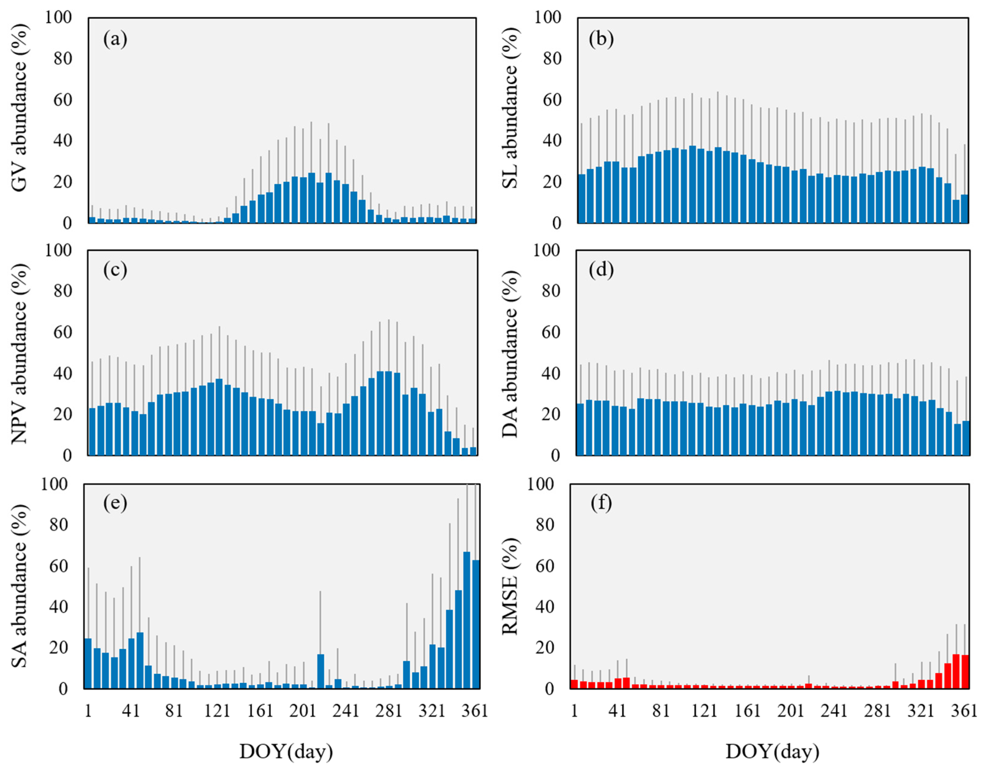
3.3. Spectral Unmixing Results and Stability Estimate

The PCA was employed to identify the characteristic seasonal patterns of endmembers over the course of a year. As shown in the eigenvalue matrix (Figure 6), (1) it is evident that the eigenvectors of PC1 predominantly maintained consistent orientations throughout most of the year (DOYs: 057–289). Notably, PC1 exhibited pronounced significance within the shortwave infrared bands, effectively amplifying the SL within the study area. Among them, the color of SL was deepest (the contribution variance reached a peak) in spring and autumn, indicating that the typical seasonal phase of SL was spring and autumn (DOYs: 113, 265–289). (2) During the period of late spring and late autumn (DOYs: 185–249), the eigenvector of PC2 showed that the near-infrared band (B4) reached a peak, indicating the PC2 in this season mainly enhanced the information of GV. (3) The eigenvector of NPV was expressed contrary to the red (B3) and NIR (B4) bands of GV. It was mainly enhanced by the PC3 of DOYs: 001–105 and 297–345 and the PC2 of DOYs: 129–177 and 257–289. Among them, the color in DOYs 145–177 was deepest, where the phase was the typical seasonal phase of NPV. (4) The eigenvector of PC2 in spring (DOYs: 089–121) showed that the direction of the visible bands and the shortwave infrared bands was opposite, indicating that it enhanced the information of SA. (5) DA, as an associated endmember, often coexisted with tall trees, mountains, and dark surfaces, and it was greatly affected by solar illumination angle. Thus, it had no fixed representative season. (6) In addition, many areas in the study area in early spring and late winter (DOYs: 001–049, 313–361) were covered with snow, and thus, the PC1 in this time period might enhance snow information. However, grassland species are hard to grow under a snow cover; therefore, snow endmember was not considered in this study.
Consequently, the standard spectral candidate sets for endmembers could be delineated using the typical seasonal phases extracted from the MOD09A1 images on DOY289, 217, 177, and 305, corresponding to SL, GV-DA, NPV, and SA, respectively. The endmembers located in each typical image were selected to assist with constructing the scatter diagrams of the corresponding representative PCs [45]. Subsequently, the average spectrum of the endmember pixel points was considered the standard spectrum (Figure 7), which was then utilized in the LSMA model for all scene images.
The endmember abundance maps of spring (DOY97), autumn (DOY209), and winter (DOY305) were visualized as an RGB composite map, revealing distinct variations across seasons (Figure 8). In the GV composite map, regions such as the Daxing’an Ling Forest, Hulun-Beir Grassland, Liaohe Plain, and Hetao Plain exhibit a vibrant green color, indicative of dense canopies during the summer months when vegetation thrives. Conversely, in areas like the Badain Jaran Desert and Tengger Desert in western Inner Mongolia, which is characterized by exposed sandy soil all year round, the composite map of SL appears white, and the composite map of NPV appears dark. In central and eastern Inner Mongolia, where sandy soil is exposed as vegetation withers, the composite maps of SL and NPV take on hues of dark purple and purple with traces of scarlet, respectively. SA is primarily distributed along the edges of oases and low-lying areas, which are exposed in both spring and winter. Meanwhile, the DA composite map exhibits increased brightness in the Badain Jaran Desert and Daxing’an Ling region. This is due to the presence of gravel in the former and extensive shadows cast by forests in the latter.
The mean abundance value, standard deviation, and root mean square error (RMSE) of the spectral unmixing are listed in Figure 9. The endmember fraction is inter-coupling, presenting the intra-annual change in vegetation growth state and soil habitat (Figure 9). The GV abundance peaked in summer, covering 20% of the total study area. In contrast to GV, NPV was more abundant in spring and autumn than in summer, and its fraction even reached 30%. The abundance of SA was small, accounting for about 10% in the study area; additionally, its higher abundance was observed in winter and spring due to agricultural practices and precipitation. However, the abundance of SA in spring and winter might be biased because the spectral spectrum of snow covers can be confused with saline-alkali land in spring and winter. Occupying a large proportion of 30%, the SL abundance slightly decreased only in summer when vegetation grew luxuriantly. Due to the solar altitude angle, DA was accompanied by mountainous and tall plants. Thus, the abundance of DA presented only a little variation across the year. The RMSE values of each seasonal scene were mostly within 0.02, with a maximum of 0.05, indicating that the unmixing results of the standard 5-endmember spectral space of GV, SL, NPV, DA, and SA performed well in Inner Mongolia with the MOD09A1 products. The RMSE value was higher in spring and winter without snow endmember, thus indicating a large amount of snow cover. However, the weak spectral trace of vegetation growth under snow cover had limited effects on the grassland extraction of the overall time series.

3.4. Accuracy Evaluation and Distribution of Grassland Types in Inner Mongolia

Given the wealth of redundant information within the time-series abundance maps, we employed PCA for dimensionality reduction (Figure 10). The results indicated that the cumulative contribution of the first 22 PCs amounted to 90%, effectively encompassing a substantial portion of surface cover characteristics and their temporal evolution.
The results of the comparative classification trials are presented in Table 1 and Table 2, showing two different input parameter configurations: one with 22 PC maps and 7 grassland occurrence probability maps (trial 1) and the other with only 22 PCs (trial 2). The overall classification accuracies for these trials were 79.43% and 74.71%, respectively, with the corresponding Kappa coefficients of 0.73 and 0.66. Compared to trial 2, the accuracy of the classification model when provided with grassland occurrence probability was improved (about 5%). Notably, the classification mainly occurred at arable land, forest, water, buildings, and bare land, which are categorized as “Other” in Table 3 and Table 4.

4. Discussion

4.1. The Results and Pattern Evolution of Grassland Classification in Inner Mongolia

As the main cover type in Inner Mongolia, grassland accounts for about 70% of the total area (82.85±3.15 × 10⁴ km2) (Figure 11). Among them, TST is the main type (accounts for 54%±0.04), which is consistent with the bio-climate zone (Figure 4a), and was primarily distributed in the center of the study area. Furthermore, a significant portion of desert-like grasslands can be found in the western part of the study area, encompassing TDT and TSDT, which together account for approximately 19%±2.2% of the total grassland area. As the typical transitional ecosystem between desert and temperate grassland, TDST mainly accounted for about 13%±2.47%. This type is roughly consistent with the boundary between temperate continental climate and temperate monsoon climate, resulting in TDST’s increased vulnerability and being easily affected by climatic disturbances such as droughts and floods. In addition, TMST, MMT, and LMT accounted for 3%±1.02%, 0.1%±0.03%, and 11%±3.19%, respectively, which showed mainly fragmented distribution on the both sides of Daxing’an Mountains in the northeastern part of the study area; their favorable light and temperature environment leads to intense species competition and better biodiversity.
We compared the classification results with the official survey map of grassland resources in the 1980s and analyzed the succession pattern of grasslands in Inner Mongolia in recent decades. China’s grassland management has undergone three waves of policy changes. The first wave occurred at the end of the 20th century when agricultural production was emphasized, and nearly 5.28±1.40 × 10⁴ km2 of grasslands was reclaimed for cultivation, primarily in the Hetao Plain and the east–northern pastoral ecotone. The second wave involved forest-based ecological restoration measures at the beginning of the 21st century. This afforestation effort resulted in the transformation of nearly 3.91±0.73 × 10⁴ km² of grassland into forested areas (Figure 12). Additionally, due to historical accumulation issues and various human activities, nearly 9.22±1.24 × 10⁴ km2 of grassland was transformed into bare lands. In the last decade, the Chinese government recognized the importance of grassland protection and has taken measures to address grassland degradation. For instance, the National Grassland Law was proposed in 2002, and the “National Forestry and Grassland Administration” was established to explore the sustainable utilization potential and ecological service function of grassland. The Inner Mongolia government has also actively implemented measures like grassland ecological compensation and adaptive grazing practices. As a result, 10.8±1.57 × 10⁴ km2 of other land had been transformed into grassland by 2019.
The grassland survey in the 1980s demanded extensive field work, and the grassland-type distribution map was achieved using field sketching and indoor supplementary drawing. The survey result map had small map spots, which eliminated most of the broken plots; however, our classification was based on pixels, which did not have the same inspection scale as the survey results. Therefore, further studies are highly needed to accurately study the evolution pattern of broken grassland types, which highlights the importance of using the same investigation standard for natural resource investigation and resource evolution analysis. However, due to the heterogeneity of spectral reflectance, it is challenging to transfer survey frameworks with different regions and scales using current RS or GIS technologies. One feasible way is to transform the original spectral space into an endmember space using the linear spectral mixture method. It can unify the dimensions of pixel signals and eliminate the application limitations of different satellite data sources [28,31,45]. Finally, the multi-scale transmission of surface cover element information can be realized, which can enhance the regional applicability of multi-scale classification frameworks. Previous studies have proved the stability and portability of SVD space for remote sensing interpretation framework.

4.2. Limitations of Classification Using MOD09A1 Imageries and Future Prospects

Our classification framework based on bio-climate indicators achieved relatively good results. However, the grassland types with sparse vegetation and broken distribution were still poorly extracted due to the 500 m spatial resolution of the MOD09A1 products. There were serious omissions of 33.33% and 46.67% PA errors for LMT and TSDT, respectively, which showed irregular and crushing distribution. Classifying TSDT and LMT grassland types posed great challenges for remote sensing analysis due to their sparse vegetation and small-scale features. The spectral signal at the 500 m spatial resolution was insufficient for accurately identifying shrubs with a diameter of 1 m–5 m when classifying TSDT. Similarly, classifying LMT located on riverbanks and depressions with perennial water bodies faced a similar dilemma. Thus, these types of grasslands demand finer spatial resolutions than temporal resolution. Therefore, finer-resolution satellite products could be highly necessary to complete a multi-scale survey framework of grassland-type identification.

4.3. Implications of the Experimental Framework with Bio-Climate Factors and SVD Space

Aside from improving mapping, our experimental framework can have broader implications and connections in the analysis of satellite data and land resource management. Firstly, because the modeling parameters are rooted in the endmember space, this framework is flexible to convert spectral signals into physical information about surface materials across different spatial resolutions using optical data. In addition, the endmember abundance maps represent the distribution of the grassland itself (including grass, soil, and moisture), while the occurrence probabilities derived from bioclimatic data indicate the suitability or conditions for grassland growth and habitat preferences. In brief, the heterogeneity among various grassland types is determined based on the differences in ecosystem integrity. Hence, this experimental framework boasts significant advantages in terms of both data adaptability and scientific applicability.
Furthermore, another aspect to consider in our framework is multi-scale analysis of land resource management. Climate data are typically employed in macro-level analyses, while multi-resolution satellite data with endmember space transformation are well-suited for addressing medium- and small-scale issues. The climate and habitat information of grasslands can help manage different grasslands at specific scales of interest, and thus, grassland landscapes can be grouped into nested hierarchies. These hierarchies are often used to describe complex systems to define entities and order landscapes at particular scales, requiring an understanding of the patterns and processes of both upscale and downscale information [51]. Information is typically passed both upscale and downscale in environmental systems, and grass landscape classification can be constructed through the process of both aggregation and subdivision (or bottom-up and top-down) [20]. Different scales of information, like climate, ecological environment, and individual vegetation units, can serve management needs for specific scales of interest (Figure 13). For example, bio-climate zoning can guide national and even global ecological strategic planning, while mapping of grassland types can guide management decisions regarding regional grassland resources. Moreover, there are further implications for employing data with a finer spatial resolution to classify smaller targets, such as a county or individual farms.

5. Conclusions

This study developed a framework for large-area grassland mapping based on the bio-climate characteristics of grasslands and the interactions of time-series endmember fraction maps. This framework is flexible and can also be applied to different regions and different ecosystems. A workflow with three phases was included in this framework. Firstly, grassland bio-climate factors were constructed using satellite-based data. Secondly, grassland occurrence probabilities were generated based on these bio-climate factors, and then different grassland bio-climate zones were identified. Finally, time-series data of vegetation-related endmembers (GV and NPV) and soil-related endmembers (SL, SA, and DA) were unmixed from the MOD09A1 images by LSMA to create grassland occurrence probability maps. Using this classification framework, a higher overall accuracy of 79.43% and a Kappa coefficient of 0.73 were achieved for mapping grasslands in Inner Mongolia. This framework could also better present a grassland generic process, including possible transitions and successions for the development of management or protective measures and policies. In addition, this study also pointed out that bio-climate characteristics could help in mapping land cover with high heterogeneity. The proposed bio-climate factor-based classification framework can provide clearer policy guidance for sensitive areas. The interpretation framework based on endmember space (SVD space) has good flexibility and can be adapted to different research areas, different data sources, and different classification scales. Finally, we also discussed the limitation of medium-resolution data for the recognition of land types with a broken surface.

Author Contributions

D.S. and M.S. designed this research study. M.S. performed the analysis. M.S., Z.J., X.J. and Q.S. processed the intra-annual time-series abundance data. M.S. and D.S. drafted the paper. F.L. polished the writing. All authors contributed to the interpretation of the results and the text. All authors have read and agreed to the published version of the manuscript.

Funding

This research was funded by the National Natural Science Foundation of China (No. 42071252 and No. 42001234).

Institutional Review Board Statement

Not applicable.

Informed Consent Statement

Not applicable.

Data Availability Statement

Data are available from the corresponding author upon request.

Conflicts of Interest

The authors declare no conflict of interest.

References

  1. Li, Y.; Brando, P.M.; Morton, D.C.; Lawrence, D.M.; Yang, H.; Randerson, J.T. Deforestation-induced climate change reduces carbon storage in remaining tropical forests. Nat. Commun. 2022, 13, 1964. [Google Scholar] [CrossRef] [PubMed]
  2. Tiedje, J.M.; Bruns, M.A.; Casadevall, A.; Criddle, C.S.; Eloe-Fadrosh, E.; Karl, D.M.; Nguyen, N.K.; Zhou, J. Microbes and Climate Change: A Research Prospectus for the Future. Mbio 2022, 13, e0080022. [Google Scholar] [CrossRef] [PubMed]
  3. Chang, Y.; Choi, D.; Kim, H. Dynamic Trends of Carbon Intensities among 127 Countries. Sustainability 2017, 9, 2268. [Google Scholar] [CrossRef]
  4. Casey, J.W.; Holden, N.M. Analysis of greenhouse gas emissions from the average Irish milk production system. Agric. Syst. 2005, 86, 97–114. [Google Scholar] [CrossRef]
  5. John, W.; Nicholas, M. Holistic analysis of GHG emissions from Irish livestock production systems. In Proceedings of the 2005 ASAE Annual Meeting, American Society of Agricultural and Biological Engineers, Tampa, FL, USA, 17–20 July 2005. [Google Scholar]
  6. Chang, J.; Ciais, P.; Gasser, T.; Smith, P.; Herrero, M.; Havlík, P.; Obersteiner, M.; Guenet, B.; Goll, D.S.; Li, W. Climate warming from managed grasslands cancels the cooling effect of carbon sinks in sparsely grazed and natural grasslands. Nat. Commun. 2021, 12, 118. [Google Scholar] [CrossRef]
  7. Garnett, T.; Godde, C.; Muller, A.; Rs, E.; Zanten, H.V. Grazed and Confused? Ruminating on Cattle, Grazing Systems, Methane, Nitrous Oxide, the Soil Carbon Sequestration Question—And What It All Means for Greenhouse Gas Emissions; FCRN: London, UK, 2017. [Google Scholar]
  8. Suttie, J.M.; Reynolds, S.G.; Batello, C. Grasslands of the World; Food & Agriculture Org.: Rome, Italy, 2005. [Google Scholar]
  9. Li, C.; Fu, B.; Wang, S.; Stringer, L.C.; Wang, Y.; Li, Z.; Liu, Y.; Zhou, W. Drivers and impacts of changes in China’s drylands. Nat. Rev. Earth Environ. 2021, 2, 858–873. [Google Scholar] [CrossRef]
  10. Ze, H.; Wei, S.; Xiangzheng, D.; Xinliang, X. Grassland ecosystem responses to climate change and human activities within the Three-River Headwaters region of China. Sci. Rep. 2018, 8, 9079. [Google Scholar]
  11. Grekousis, G.; Mountrakis, G.; Kavouras, M. An overview of 21 global and 43 regional land-cover mapping products. Int. J. Remote Sens. 2015, 36, 5309–5335. [Google Scholar] [CrossRef]
  12. Smith, W.K.; Dannenberg, M.P.; Yan, D.; Herrmann, S.; Yang, J. Remote sensing of dryland ecosystem structure and function: Progress, challenges, and opportunities. Remote Sens. Environ. 2019, 233, 111401. [Google Scholar] [CrossRef]
  13. Chladil, M.A.; Nunez, M. Assessing Grassland Moisture and Biomass in Tasmania-the Application of Remote-Sensing and Empirical-Models for a Cloudy Environment. Int. J. Wildland Fire 1995, 5, 165–171. [Google Scholar] [CrossRef]
  14. McVicar, T.R.; Jupp, D.L. The current and potential operational uses of remote sensing to aid decisions on drought exceptional circumstances in Australia: A review. Agric. Syst. 1998, 57, 399–468. [Google Scholar] [CrossRef]
  15. Hazaymeh, K.; Hassan, Q.K. A remote sensing-based agricultural drought indicator and its implementation over a semi-arid region, Jordan. J. Arid Land 2017, 9, 319–330. [Google Scholar] [CrossRef]
  16. Belda, M.; Holtanová, E.; Halenka, T.; Kalvová, J. Climate classification revisited: From Köppen to Trewartha. Clim. Res. 2014, 59, 1–13. [Google Scholar] [CrossRef]
  17. Peel, M.C.; Finlayson, B.L.; Mcmahon, T.A. Updated World Map of the Koppen-Geiger Climate Classification. Hydrol. Earth Syst. Sci. 2007, 11, 1633–1644. [Google Scholar] [CrossRef]
  18. Jing, H.; Feng, Y.; Zhang, W.; Zhang, Y.; Chen, K. Effective Classification of Local Climate Zones Based on Multi-Source Remote Sensing Data. In Proceedings of the IGARSS 2019—2019 IEEE International Geoscience and Remote Sensing Symposium, Yokohama, Japan, 28 July–2 August 2019. [Google Scholar]
  19. Du, L.; Tian, Q.; Yu, T.; Meng, Q.; Jancso, T.; Udvardy, P.; Huang, Y. A comprehensive drought monitoring method integrating MODIS and TRMM data. Int. J. Appl. Earth Obs. Geoinf. 2013, 23, 245–253. [Google Scholar] [CrossRef]
  20. Salley, S.; Talbot, C.J.; Brown, J. The Natural Resources Conservation Service Land Resource Hierarchy and Ecological Sites. Soil Sci. Soc. Am. J. 2016, 80, 1–9. [Google Scholar] [CrossRef]
  21. van de Vlag, D.E.; Stein, A. Incorporating Uncertainty via Hierarchical Classification Using Fuzzy Decision Trees. IEEE Trans. Geosci. Remote Sens. 2007, 45, 237–245. [Google Scholar] [CrossRef]
  22. Ricotta, C. The influence of fuzzy set theory on the areal extent of thematic map classes. Int. J. Remote Sens. 1999, 20, 201–205. [Google Scholar] [CrossRef]
  23. Bazi, Y.; Melgani, F. Gaussian Process Approach to Remote Sensing Image Classification. IEEE Trans. Geosci. Remote Sens. 2010, 48, 186–197. [Google Scholar] [CrossRef]
  24. Xie, Q.; Peng, K. Space-Time Distribution Laws of Tunnel Excavation Damaged Zones (EDZs) in Deep Mines and EDZ Prediction Modeling by Random Forest Regression. Adv. Civ. Eng. 2019, 2019, 1–13. [Google Scholar] [CrossRef]
  25. Zhang, L.; Wu, X.; Ji, W.; Abourizk, S.M. Intelligent Approach to Estimation of Tunnel-Induced Ground Settlement Using Wavelet Packet and Support Vector Machines. J. Comput. Civil. Eng. 2016, 31, 4016053. [Google Scholar] [CrossRef]
  26. Li, N.; Jimenez, R. A logistic regression classifier for long-term probabilistic prediction of rock burst hazard. Nat. Hazards 2018, 90, 197–215. [Google Scholar] [CrossRef]
  27. Qiangqiang, S.; Ping, Z.; Danfeng, S.; Aixia, L.; Jianwang, D. Desert vegetation-habitat complexes mapping using Gaofen-1 WFV (wide field of view) time series images in Minqin County, China. Int. J. Appl. Earth Obs. Geoinf. 2018, 73, 522–534. [Google Scholar]
  28. Small, C.; Milesi, C. Multi-scale standardized spectral mixture models. Remote Sens. Environ. 2013, 136, 442–454. [Google Scholar] [CrossRef]
  29. Sun, D.; Zhang, P.; Sun, Q.; Jiang, W. A dryland cover state mapping using catastrophe model in a spectral endmember space of OLI: A case study in Minqin, China. Int. J. Remote Sens. 2019, 40, 5673–5694. [Google Scholar] [CrossRef]
  30. Sun, Q.; Zhang, P.; Jiao, X.; Lun, F.; Dong, S.; Lin, X.; Li, X.; Sun, D. A Remotely Sensed Framework for Spatially-Detailed Dryland Soil Organic Matter Mapping: Coupled Cross-Wavelet Transform with Fractional Vegetation and Soil-Related Endmember Time Series. Remote Sens. 2022, 14, 1701. [Google Scholar] [CrossRef]
  31. Sun, M.; Jiao, X.; Ji, Z.; Shi, L.; Zhan, Y.; Li, L.; Han, W.; Sun, D. Grassland system cognitive theory and its spectral identification method. China Land Sci. 2022, 36, 84–95. [Google Scholar]
  32. Fensholt, R.; Rasmussen, K.; Kaspersen, P.; Huber, S.; Horion, S.; Swinnen, E. Assessing Land Degradation/Recovery in the African Sahel from Long-Term Earth Observation Based Primary Productivity and Precipitation Relationships. Remote Sens. 2013, 5, 664–686. [Google Scholar] [CrossRef]
  33. Sun, D. Detection of dryland degradation using Landsat spectral unmixing remote sensing with syndrome concept in Minqin County, China. Int. J. Appl. Earth Obs. Geoinf. 2015, 41, 34–45. [Google Scholar] [CrossRef]
  34. Sun, Q.; Zhang, P.; Jiao, X.; Han, W.; Sun, D. Identifying and understanding alternative states of dryland landscape: A hierarchical analysis of time series of fractional vegetation-soil nexuses in China’s Hexi Corridor. Landsc. Urban Plan. 2021, 215, 104225. [Google Scholar] [CrossRef]
  35. Lingtong, D.; Qingjiu, T.; Yan, H.; Jun, L. Drought monitoring based on TRMM data and its reliability validation in Shandong province. Trans. Chin. Soc. Agric. Eng. 2012, 28, 121–126. [Google Scholar]
  36. Chen, S.; Zhang, L.; Guo, M.; Liu, X. Suitability analysis of TRMM satellite precipitation data in regional drought monitoring. Nongye Gongcheng Xuebao/Trans. Chin. Soc. Agric. Eng. 2018, 34, 126–132. [Google Scholar]
  37. Wei, W.; Pang, S.; Wang, X.; Zhou, L.; Li, C. Temperature Vegetation Precipitation Dryness Index (TVPDI)-based dryness-wetness monitoring in China. Remote Sens. Environ. 2020, 248, 111957. [Google Scholar] [CrossRef]
  38. Kang, J.; Yang, X.; Wang, Z.; Huang, C.; Wang, J. Collaborative Extraction of Paddy Planting Areas with Multi-Source Information Based on Google Earth Engine: A Case Study of Cambodia. Remote Sens. 2022, 14, 1823. [Google Scholar] [CrossRef]
  39. Li, W.; Dong, R.; Fu, H.; Wang, J.; Yu, L.; Gong, P. Integrating Google Earth imagery with Landsat data to improve 30-m resolution land cover mapping. Remote Sens. Environ. 2020, 237, 111563. [Google Scholar] [CrossRef]
  40. Xie, S.; Liu, L.; Zhang, X.; Yang, J.; Chen, X.; Gao, Y. Automatic Land-Cover Mapping using Landsat Time-Series Data based on Google Earth Engine. Remote Sens. 2019, 11, 3023. [Google Scholar] [CrossRef]
  41. Wang, Z.; Wang, Z.; Xiong, J.; He, W.; Yong, Z.; Wang, X. Responses of the Remote Sensing Drought Index with Soil Information to Meteorological and Agricultural Droughts in Southeastern Tibet. Remote Sens. 2022, 14, 6125. [Google Scholar] [CrossRef]
  42. Li, T.; Lü, Y.; Fu, B.; Comber, A.J.; Harris, P.; Wu, L. Gauging policy-driven large-scale vegetation restoration programmes under a changing environment: Their effectiveness and socio-economic relationships. Sci. Total Environ. 2017, 607–608, 911–919. [Google Scholar] [CrossRef]
  43. Sun, D.; Liu, N. Coupling spectral unmixing and multiseasonal remote sensing for temperate dryland land-use/land-cover mapping in Minqin County, China. Int. J. Remote Sens. 2015, 36, 3636–3658. [Google Scholar] [CrossRef]
  44. Adams, J.B.; Sabol, D.E.; Kapos, V.; Filho, R.A.; Roberts, D.A.; Smith, M.O.; Gillespie, A.R. Classification of multispectral images based on fractions of endmembers: Application to land-cover change in the Brazilian Amazon. Remote Sens. Environ. 1995, 52, 137–154. [Google Scholar] [CrossRef]
  45. Small, C. The Landsat ETM+ spectral mixing space. Remote Sens. Environ. 2004, 93, 1–17. [Google Scholar] [CrossRef]
  46. Oreski, D.; Oreski, S.; Klicek, B. Effects of dataset characteristics on the performance of feature selection techniques. Appl. Soft Comput. 2017, 52, 109–119. [Google Scholar] [CrossRef]
  47. Loh, W.Y. Classification and regression trees. Wires Data Min. Knowl. Discov. 2011, 1, 14–23. [Google Scholar] [CrossRef]
  48. Breiman, L. Random forests. Mach. Learn. 2001, 45, 5–32. [Google Scholar] [CrossRef]
  49. Rodriguez-Galiano, V.F.; Ghimire, B.; Rogan, J.; Chica-Olmo, M.; Rigol-Sanchez, J.P. An assessment of the effectiveness of a random forest classifier for land-cover classification. Isprs-J. Photogramm. Remote Sens. 2012, 67, 93–104. [Google Scholar] [CrossRef]
  50. Olofsson, P.; Foody, G.M.; Herold, M.; Stehman, S.V.; Woodcock, C.E.; Wulder, M.A. Good practices for estimating area and assessing accuracy of land change. Remote Sens. Environ. 2014, 148, 42–57. [Google Scholar] [CrossRef]
  51. Bestelmeyer, B.T.; Brown, J.R.; Fuhlendorf, S.D.; Fults, G.; Wu, X.B. A Landscape Approach to Rangeland Conservation Practices; USDA Agricultural Research Service: Washington, DC, USA, 2011.
Figure 1. Study area and distribution of grassland field types. Photos of MMT, TMS, and LMT were captured by Zhengxin Ji in 2021, while photos of TDT and TST were taken by Minxuan Sun in 2019, and images of TSDT and TDST were sourced from national grassland special survey (NGSS) database.
Remotesensing 15 04723 g001
Figure 2. The flow chart of grassland type mapping framework.
Remotesensing 15 04723 g002
Figure 3. China Grassland Type Classification System: (a) The 3D spatial distribution of CGTCS, with moisture, temperature, and altitude indicating the three dimensions. The dotted lines show the types that our study used. (b) A list of the full names of each type.
Remotesensing 15 04723 g003
Figure 4. (a) The grassland generic probability distribution maps. (bh) are generic probabilities of TDT, TDST, TST, TSDT, TMST, MMT, and LMT, respectively.
Remotesensing 15 04723 g004
Figure 5. The critical transition zones and latent succession of desert-to-steppe and steppe-to-meadow transition.
Remotesensing 15 04723 g005
Figure 6. Principal component load factor matrix and variance contribution rate.
Remotesensing 15 04723 g006
Figure 7. Standard endmembers spectral reflectance. Shade area represents the interval of standard deviation. Endmember.
Remotesensing 15 04723 g007
Figure 8. Three temporal false-color composite images, where red, green, and blue represent the respective average endmember fractional abundance in spring (DOY: 97), summer (DOY: 209), and early winter (DOY: 305) for green vegetation (GV, (a)), sand land (SL, (b)), non-photosynthetic vegetation (NPV, (c)), saline land (SA, (d)), and dark surfaces (DA, (e)).
Remotesensing 15 04723 g008
Figure 9. Statistics of endmember abundances and LSMA results: (ae) the average abundance of green vegetation (GV), sand land (SL), non-photosynthetic vegetation (NPV), dark surfaces (DA), and saline land (SA), respectively, and (f) indicates the RMSE. The gray lines are standard deviations.
Remotesensing 15 04723 g009
Figure 10. The eigenvalues and the contributions of principal components (PCs) after dimensionality reduction in the abundance maps. Accuracy of land-use cover classification with different percentages of contribution of the PCs.
Remotesensing 15 04723 g010
Figure 11. Results of classification: (a) without grassland occurrence probability; (b) with grassland occurrence probability.
Remotesensing 15 04723 g011
Figure 12. Statistics of grassland evolution in Inner Mongolia since the 1980s.
Remotesensing 15 04723 g012
Figure 13. Hierarchy of grassland ecological resource (bottom), mapping (upper left), and management (upper right).
Remotesensing 15 04723 g013
Table 1. Satellite-based data information.
Data TypeProduction/TileSpatial
Resolution
Temporal Resolution/UnitDescriptionSource
MODIS
(Terra/Aqua)
MOD09A1500 m (2019)8-DayGrassland type mappinghttp://modis.gsfc.nasa.gov (accessed
on 1 June 2021)
MOD11A2 LST1 km (2001–2019)8-Day/°CGrassland genesis factors and potential vegetation zoning
MOD13A3 NDVI1 km (2001–2019)Monthly
TRMMTRMM 3B43
precipitation
0.25° (2001–2019)mm/h
STRMSTRM DEM 90 m-https://earthexplorer.usgs.gov (accessed on 2 March 2021)
Table 2. The specific quantitative strategies of grassland bio-climate factors.
CategoryFactorsData SourceTimeQuantitative Process
Land surface temperature (LST)Temperature of the warmest monthMOD11A2 LST2001–2019Based on the 8-day time-series data, calculate the mean value of daytime temperature in July across 19 years
Temperature of the coldest monthMOD11A2 LST2001–2019Based on the 8-day time-series data, calculate the mean value of daytime temperature in January across 19 years
Accumulated temperature of >0 °CMOD11A2 LST2001–2019Based on the 8-day time-series data, calculate the accumulated temperature when the daytime temperature is greater than 0 °C across 19 years
Land surface moisture
(TVPDI)
TemperatureMOD11A2 LST2001–2019Based on the 8-day time-series data, calculate the mean value of daytime temperature across 19 years
VegetationMOD13A3 NDVI2001–2019Based on the monthly time-series data, calculate the mean value of NDVI across 19 years
PrecipitationTRMM 3B432001–2019Based on the monthly time-series data, calculate the mean value of precipitation across 19 years and then downscale to 1 km
TopographicAltitudeSTRM DEM--
MoistureTVPDI--
Table 3. Accuracy of grassland type classification based on grassland bio-climate indicators.
TypeMMTLMTTMSTTSTTDSTTSDTTDTOther
MMT166200002
LMT27000002
TMST1519100000
TST01912952121
TDST000350118
TSDT00010701
TDT000023224
Other0208024171
PA (%)84.2133.3363.3385.4387.7246.6778.5781.82
UA (%)61.5463.6454.2976.7979.3777.7870.9791.44
Overall accuracy (%): 79.43%; Kappa: 0.73.
Table 4. Accuracy of direct classification of grassland types.
TypeMMTLMTTMSTTSTTDSTTSDTTDTOther
MMT111100001
LMT512000000
TMST11850002
TST2520129101319
TDST000742329
TSDT00011100
TDT000028194
Other0219224174
PA (%)57.8957.1426.6785.4373.686.6767.8683.25
UA (%)78.5770.5947.0668.2566.6733.3357.5889.69
Overall accuracy (%): 74.71%; Kappa: 0.66.
Disclaimer/Publisher’s Note: The statements, opinions and data contained in all publications are solely those of the individual author(s) and contributor(s) and not of MDPI and/or the editor(s). MDPI and/or the editor(s) disclaim responsibility for any injury to people or property resulting from any ideas, methods, instructions or products referred to in the content.

