Article

Spatiotemporal Variation of Anticyclonic Eddies in the South China Sea during 1993–2019

1
State Key Laboratory of Marine Environmental Science, Center for Marine Meteorology and Climate Change, College of Ocean and Earth Sciences, Xiamen University, Xiamen 361102, China
2
Southern Marine Science and Engineering Guangdong Laboratory (Zhuhai), Zhuhai 519082, China
*
Author to whom correspondence should be addressed.
Remote Sens. 2023, 15(19), 4720; https://doi.org/10.3390/rs15194720
Submission received: 31 July 2023 / Revised: 2 September 2023 / Accepted: 21 September 2023 / Published: 27 September 2023
(This article belongs to the Special Issue Remote Sensing Applications in Ocean Observation II)

Abstract

:
Based on the absolute dynamic topography data from the Copernicus Marine Environment Monitoring Service, this paper applies the Topographic Position Index to develop a new approach for mapping the anticyclonic eddies in the South China Sea (SCS). The results show that anticyclonic eddies are active in the deep basin of SCS, and the five selected parameters (number or frequency, lifetime, kinetic energy, amplitude, and area or radius) of anticyclonic eddies have a similar temporal variation and a similar spatial distribution pattern. (1) As for monthly variations, anticyclonic eddies are active in late spring and most active in summer. (2) The El Niño–Southern Oscillation had a stronger impact on the inter-annual variations of anticyclonic eddies in the SCS before 2013, resulting in a significant transition of inter-annual variations of these five parameters in around 2004. After 2013, most of these five parameters had a minimum in 2015 and a maximum in 2017. (3) Analyses show that the eddy activities in the SCS are significantly influenced by the monsoon wind and the western boundary current like Kuroshio. Therefore, the areas southwest of Taiwan Island and east of Vietnam are the two areas where the anticyclonic eddies are most active, with much larger eddy kinetic energy and much higher eddy amplitude.

1. Introduction

The South China Sea (SCS) is the largest semi-closed marginal sea in the northwestern Pacific (Figure 1a). To the north, south and west, the SCS is surrounded by lands; to the east, the Luzon Strait connects the SCS with the Pacific Ocean. Currents in the SCS are largely influenced by the monsoon and show significant seasonal variations (Figure 1b–e). The shelf water moves northward in summer, while the opposite happens in winter. To the northeast of SCS, there exists a strong western boundary current “Kuroshio” all year round. In the south of SCS, the “Nansha upper anticyclone” appears in winter (about 110°–115°E, 5°–9°N in Figure 1e) [1]. These currents create favorable conditions for eddy generation. The total area of SCS is about 3.5 × 10⁶ km2, and the maximum depth is more than 5000 m, with an average depth of more than 1000 m. Such a large scale makes the SCS suitable for eddy generation and propagation [2]. Mesoscale eddy is an important phenomenon in the SCS [3,4] and plays a key role in the transport of heat (and salt) and the variation of dynamic conditions [5].
There have been plenty of studies focusing on the eddies in the SCS. Zheng et al. [2] reviewed the research process of mesoscale eddy in the SCS in detail. From the 1960s to the mid-1990s, based on the observation data, the studies about eddies in the SCS mainly reported the existence of an individual eddy, described the characteristics and explained the dynamic mechanisms of each individual eddy in the SCS.
In the 21st century, with the development of satellite remote sensing, it became possible to use remote sensing data to study the spatiotemporal variation and distribution of eddies. In recent years, lots of eddy-detection methods have been promoted. For example, the Okubo–Weiss (O-W) parameter [6], the closed contour method [7,8,9], the vector-geometry [10] and the winding-angle algorithms [11] are widely used to map eddies. Also, the machine learning method was applied to the eddy mapping, e.g., [12]. There have been some studies focusing on eddies in the SCS. Wang et al. [3] used 8-year (1993–2000) Sea Level Anomaly (SLA) data to statistically analyze the spatiotemporal variation of mesoscale eddies lasting for more than 60 days in the SCS. They found 86 long-term mesoscale eddies in total (28 cyclonic eddies, and 58 anticyclonic eddies), and the northeast of the SCS deep basin, the west of Luzon Strait and the western boundary of the deep basin are the areas where eddies occur frequently. Using the SLA data from “Archiving, Validation and Interpretation of Satellite Oceanographic data” (AVISO), setting the shortest lifetime of the eddy to be 35 days, Lin et al. [13] found more eddies during 1993–2002 and then studied the variation of eddy characteristics in the SCS. Based on 15-year remote sensing data and O-W parameter, Xiu et al. [14] analyzed the eddy number, eddy frequency and eddy kinetic energy by comparing the results from satellite remote sensing data and the results from the Regional Ocean Model System (ROMS). They made a systematic summary of the features of eddies in the SCS. But limited to the time resolution, the shortest eddy lifetime was also limited to 30 days. Combining the 17-year (from October 1992 to October 2009) AVISO data and Argo data, Chen et al. [5] discussed how eddies influence the ocean thermal vertical structure. Based on the O-W parameter and other additional restrictions, Du et al. [15] analyzed the features of eddies in the SCS during 1992–2012. They found that the merging and splitting of eddies were active in the northwest of Luzon Strait. Using the eddy product derived from two-satellite merged data, combining large amounts of Argo data, He et al. [16] investigated the surface features, 3D structure and heat transport of eddy from 1993 to 2015.
Limited to the time resolution (time step is 7 days in general), eddies with a lifetime of more than 28 days (or more, four time-steps at least) were considered in most previous studies. Thus, the eddies with short lifetimes were ignored and their high-frequency variation was also filtered. The studies mentioned above did not separate out the anticyclonic eddies and cyclonic eddies. Some studies focused on the cyclonic eddies in the SCS, as upwelling would transport nutrient-rich water to the surface/subsurface at the center of cyclonic eddies, resulting in high phytoplankton biomass and high primary production [17,18]. But actually, the distributions of zooplankton and phytoplankton are also strongly influenced by the edge effects (which are dominated by submesoscale instabilities) of anticyclonic eddies in the SCS [19]. This effect did not attract much attention because of the lack of high-resolution observations or model simulations. As there is a lot of focus on the submesoscale instabilities which usually appear on the edge of anticyclonic eddies, a census study of anticyclonic eddies in the SCS is indispensable.
Based on the altimetry data provided by Copernicus Marine Environment Monitoring Service (CMEMS), a new parameter is selected to map anticyclonic eddies in the SCS and the short-term eddies that have been neglected before are also tracked. According to the census study, we can have a more comprehensive understanding of the features of anticyclonic eddies in the SCS.

2. Data and Methods

2.1. Data

Twenty-seven years (from 1993 to 2019) of daily Absolute Dynamic Topography (ADT) and sea surface geostrophic current velocity data from CMEMS are used to detect, track anticyclonic eddies and calculate the characteristics of anticyclonic eddies in the SCS. The gridded ADT data were produced by merging these along-tracking altimeter products, including Jason-3, Sentinel-3A, Haiyang-2A, Saral/Altika, Cryosat-2, Jason-2, Jason-1, TOPEX/Poseidon, Envisat, Geosat Follow-On (GFO), and European Remote-Sensing Satellites (ERS-1 and ERS-2). The spatial resolution of the data is 0.25° × 0.25° and the time resolution is 1 day. The data have been used to detect eddies in the global ocean [8] and fronts in the SCS [20]. To obtain the finer surface features of anticyclonic eddy, the data are interpolated to 1/16° × 1/16° in this study.
Climate Forecast System and Climate Forecast System version 2 wind field data from the National Centers for Environmental Prediction (NCEP) are adapted to calculate the wind stress curl. The climatologically mean temperature fields (World Ocean Altas 2018, WOA2018) and ocean Niño Index, which are used to calculate the Rossby radius of deformation and to analyze the relationship between El Niño–Southern Oscillation and the eddy activities in the SCS, are obtained directly from National Oceanic and Atmospheric Administration (NOAA).

2.2. Eddy Detection Method

Anticyclonic (cyclonic) eddies are featured with positive (negative) local anomalies of ADT. In this paper, the Topographic Position Index (TPI) is calculated to directly represent the ADT anomaly, so as to detect the anticyclonic eddies in the SCS.

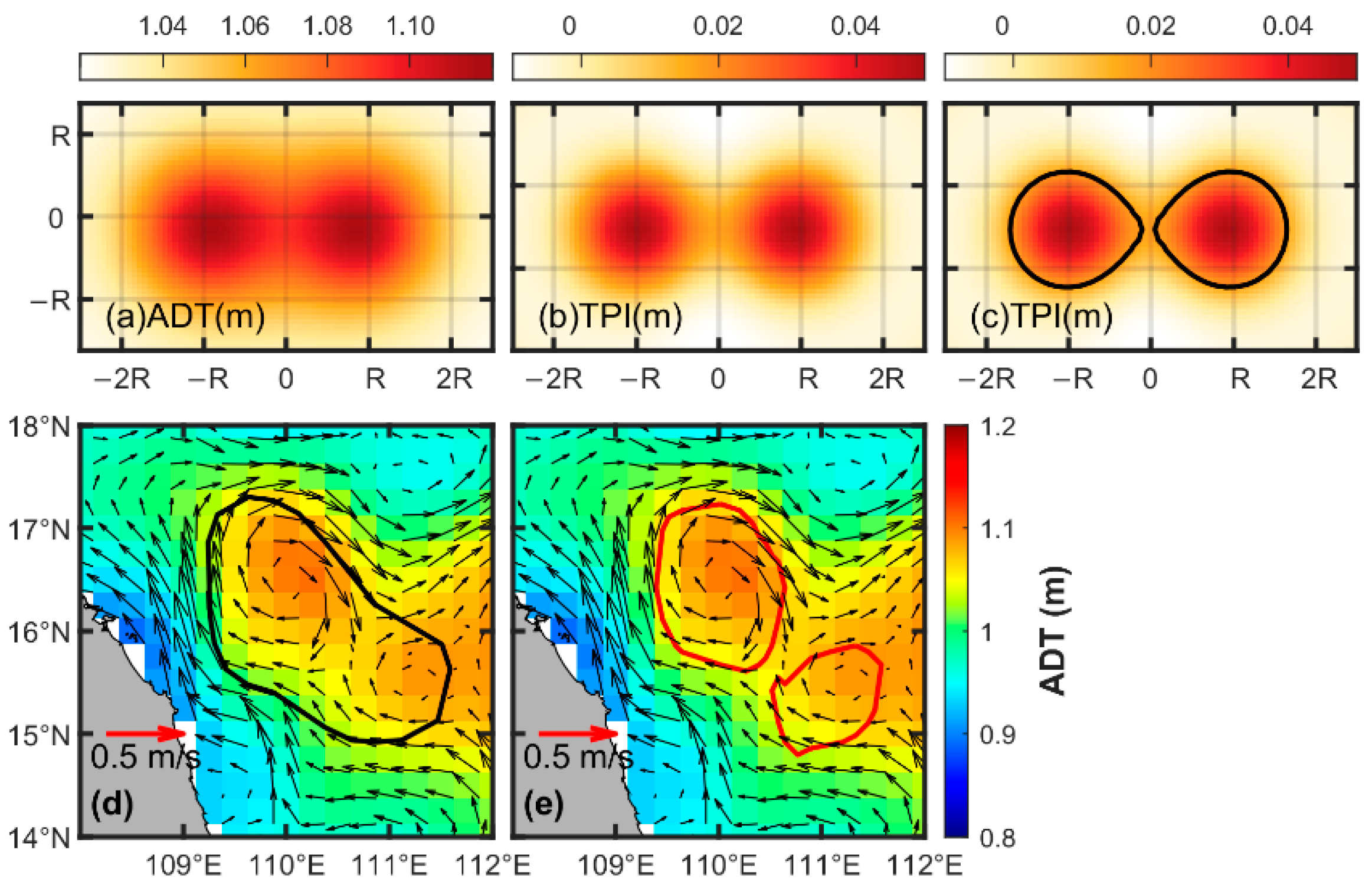
2.2.1. Topographic Positioning Index Calculation

The first step is to calculate the TPI from an ADT image (Figure 2a,b). TPI is a local-based algorithm that calculates the difference between the center cell and its neighbors, which was first used to classify landform types [21]. The TPI has been successfully used to map the ocean currents [22,23] and upwelling [24,25,26]. In this study, TPI represents the local anomaly of ADT data. The TPI parameter is calculated using the following equation:
TPI ( x , y ) = ADT ( x , y ) WD ( x , y )
where x and y are the positions of the center cell, and WD(x,y) is the mean ADT within a nominated window surrounding the center cell. In this study, we use a circle window with a radius of about 150 km (24 ADT image cells), which is deemed larger than the radius of most eddies in the SCS.

2.2.2. Eddy Detection Procedure

Closed TPI contours are deemed as potential eddies satisfying the following conditions:
(1)
The closed contours must be circle-like or ellipse-like and pass a shape test with the shape-error ≤55% (circle-like) or 40% (ellipse-like). In this study, the shape-error is defined as the ratio between the areal sum of deviations (the area difference of the closed TPI contour and its fitted circle or ellipse) and the area of that fitted circle (or ellipse).
(2)
The number of pixels within the closed contour must be larger than 64 (i.e., area ≥ 400 km2) and less than 10240 (i.e., area ≤ 400,000 km2).
(3)
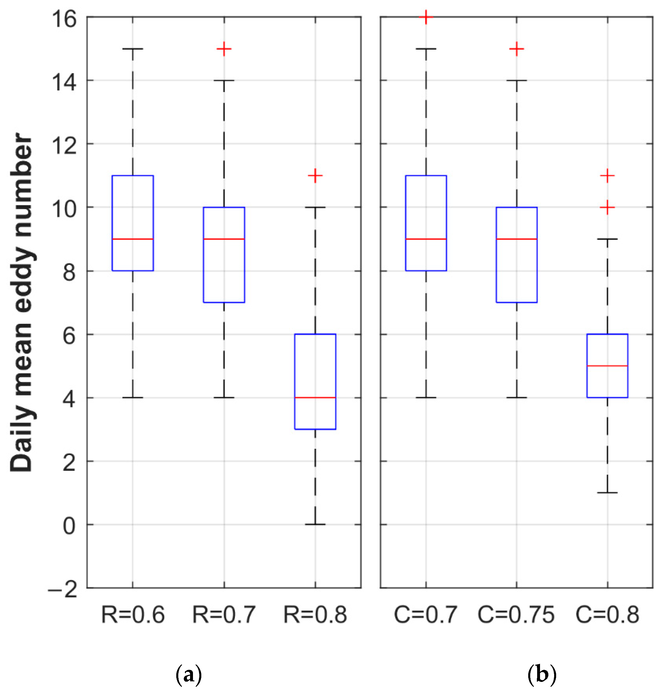
The roundness of the closed contour should be larger than 0.7 and the convexity of the closed contour should be larger than 0.75. Roundness larger than 0.7 would make the closed contour look smoother, and the convexity larger than 0.75 would keep only one eddy in the closed contour [27].
(4)
The amplitude (the difference between the mean ADT of the edge and the maximum ADT of the structure within the closed contour) should be larger than 1 cm.
Most parameters listed above are the typical values chosen in previous studies, e.g., [5,8,28]. The roundness and convexity may be two relatively new parameters in the eddy mapping method, and both of them have passed the sensitivity experiments. The results of the sensitivity experiments are summarized in Figure 3. In the first experiment (Figure 3a), we keep convexity constant (C = 0.75), while varying roundness (R) from 0.6 to 0.7 and to 0.8. In the second experiment (Figure 3b), we keep roundness constant (R = 0.7) while varying convexity (C) from 0.7 to 0.75 and to 0.8. It should be noted that all other parameters remained constant in the sensitivity analyses. It can be seen that the daily mean eddy number detected by our method is sensitive to these two parameters only when they are large enough. When the Roundness is less than or equal to 0.7, the daily mean number of eddies detected by our method does not change greatly, while R = 0.8 would largely reduce the daily mean eddy number. Though we want to find eddies that are circle-like, studies also show that eddies are not all the shape of a circle, e.g., [29]. So we tend to choose R = 0.7 as the threshold to make sure that eddy candidates with odd shapes would be removed while most of the eddy candidates can be retained for our analyses. For the same reason, the convexity was selected to be 0.75.
To catch all anticyclonic eddies of different ADT fields in the SCS, we calculate TPI contours starting from 0.01 to the maximum of TPI at an interval of 1% TPI-maximum.
Once a region is identified as an eddy candidate, the pixels within it would be removed from the TPI image, making these pixels unavailable for further eddy identification.

2.2.3. Eddy Tracking Method

Since the day-to-day general displacement of mesoscale eddies does not exceed 10 km [28], the overlap method is adopted. The overlap method has been used to track eddies in some previous studies and shows its advantages, e.g., [30,31,32,33]. Note, that eddies appearing in the area shallower than 100 m would be removed from the statistics as the ADT data are influenced heavily by the tides and internal waves there [5]. The tracking procedure is described as follows:
In the first step, eddy A at time step t should be overlapped with eddy B at time step t + dt.
Second, the overlap ratio must be larger than 5% where the overlap ratio is defined as the overlap area divided by the area of eddy A. Such a small overlap ratio would make sure that we can track small eddies splitting from (or merging into) large eddies. Actually, over 97% of the eddies have an overlap ratio greater than 50%, over 90% of the eddies have an overlap ratio greater than 75% and only about 0.6% of the eddies have an overlap ratio less than 20% in our results.
Third, only eddies lasting for more than 10 days are retained. The 10-day cut-off has been used in previous studies and is deemed as a valid cut-off. The all-satellites merged product used in this study is constructed by all the available satellite data at a given time. Due to the diversity of the track’s location and the different repetition periods of the altimetric missions, the small-scale change in the ocean activities is believed to be contained in the data [28]. Therefore, mesoscale eddies retrieved from these products are thus improved at small scales. Most previous studies set the shortest eddy lifetime to be 28 days, e.g., [7] which is due to the weekly availability of the altimetry maps. Pegliasco et al. [28] had shown that eddies with a lifetime between 10 and 30 days (called short-term eddies) also exhibit the same structures and features as eddies with a lifetime longer than 30 days. For this reason, the shortest lifetime was set to be 10 days. Due to the noise and other errors in the ADT data or due to the restrictions of the mapping procedure [9,28], eddies may “disappear” for one or two (even more) days, and then reappear again later. To address this problem, we allow eddies to “disappear” for 4 days at most.

2.3. Accuracy and Advantages

2.3.1. Accuracy

To see if our results are reliable, we compare our results with two well-known eddy datasets: the MESOSCALE EDDY TRAJECTORIES ATLAS PRODUCT META3.2EXP NRT provided by the AVISO [28] and the near-Global Ocean Mesoscale Eddy Atmospheric-Oceanic-Biological Interaction Observational Dataset (GOMEAD) provided by the Science Data Bank [34]. The results show that our results have a good agreement with these two data sets. Take eddies in 2018 for example, there were 3770 anticyclonic eddies detected by the AVISO in 2018 (amplitude larger than 1 cm), 1157 anticyclonic eddies detected by GOMEAD (lifetime longer than 28 days), and 4108 anticyclonic eddies detected by our method. Because of the different eddy lifetime cut-offs, the number of eddies detected by AVISO is different from the number of eddies detected by GOMEAD. Among all the eddies detected by the AVISO, 70.3% of which can be captured by our method, while among the 1157 eddies provided by GOMEAD, 79.3% of which can be captured by our method. It can be seen that most eddies detected by the AVISO or GOMEAD can also be detected by our method. In this case, we believe the results detected by our method are reliable.

2.3.2. Advantages and Limitations

TPI is a local-based algorithm and it represents the local anomaly of the ADT here. In this case, it would be easier to separate eddies who are very close using TPI. As shown in Figure 4a–c, we construct two anticyclonic eddies that are very close to each other (presented as two positive ADT highs). When we apply our method to detect these two eddies, it can be seen that these two eddies are well separated by our method (black lines in Figure 4c). An example in the real ocean is given in Figure 4d,e. In Figure 4d, the black line indicates the eddy boundary detected by AVISO, while from the sea surface geostrophic currents we can see that there are two anticyclonic eddies within the black line. Figure 4e shows that these two eddies are successfully identified by our method. This indicates that our method has the advantage of detecting eddies that are very close to each other. However, our method also has some limitations. For example, some studies, e.g., [35,36] have shown that some eddies have negatively correlated SSH–SST relationships. These eddies can be also found in the SCS. However, we cannot distinguish these eddies using our method for now, and this method will be improved in the future. As a census study about the anticyclonic eddies in the SCS, we believe the eddies mapped by this method can reflect the basic features of normal anticyclonic eddies in the SCS.

2.4. Statistics of Eddy Characteristics

2.4.1. Eddy Kinetic Energy Calculation

Eddy kinetic energy (EKE) is produced by the perturbations of the surface velocity and is thought to be dynamically related to eddy activities [14]. EKE can be used to measure the strength of the mesoscale activities [37], and it can be calculated by the equation below:
E K E = 1 2 ( U g 2 + V g 2 ) ¯
where the E K E is the eddy kinetic energy, the U g 2 and V g 2 are the zonal and meridional components of the geostrophic velocity anomalies which are referenced to the mean geostrophic velocity from 1993 to 2012. The U g and V g used in this study are directly obtained from the CMEMS.

2.4.2. Other Characteristics

Besides the EKE, four other characteristics of anticyclonic eddies are also analyzed in this study, namely, eddy number (eddy frequency for spatial distribution), total area (eddy radius for spatial distribution), eddy lifetime and eddy amplitude (as defined above). The eddy number in this study is the eddy trajectory number. Note here, if one eddy lasts from one month (season/year) to the next month (season/year), the monthly (seasonal/annual) mean eddy number would take it into account twice. The eddy frequency is the occurrence possibility of eddy in the corresponding area. The total area is the sum area of all anticyclonic eddies in the SCS. As for the spatial distribution, the eddy radius (calculated by a / p i , where a is the area of that eddy) is chosen to represent the eddy area. The monthly (seasonal/annual) mean eddy lifetime is defined as the lasting time of eddy generated in the corresponding month (season/year).

3. Results

3.1. Temporal Variations of Anticyclonic Eddy Characteristics

3.1.1. Temporal Variations of Anticyclonic Eddy Number

From 1993 to 2019, there were 4492 anticyclonic eddies (whose lifetime is more than 10 days) in the SCS, with about 166 anticyclonic eddies per year on average (Figure 5a). Because the shortest lifetime of eddy is limited to 10 days, the eddy number detected in this study is much more than the results of previous studies. The variation in the annual mean eddy number from 1993 to 2019 is shown in Figure 5a. Anticyclonic eddies occurred most frequently in 2008 and 2009 (193 anticyclonic eddies in both years). In 2012, the minimum annual mean eddy number appeared, with 155 anticyclonic eddies only. As shown in Figure 5b, the monthly mean eddy number of anticyclonic eddies increases from January and February, reaching the maximum in May (~28.1 anticyclonic eddies on average), and then decreases till November and December. As for seasonal variation (Figure 5c), the anticyclonic eddy number in the SCS is largest in spring (March, April and May), and then gradually decreases to the minimum in the winter (December, January and February).

3.1.2. Temporal Variations of Anticyclonic Eddy Lifetime

Among the 4492 anticyclonic eddies trajectories, the shortest lifetime of all eddies is 10 days (the shortest lifetime limited by the tracking method) and the longest lifetime is 198 days (from 19 April to 23 October 2017). The eddy with the longest lifetime appeared east of Hainan Island, moving in the range of 112°–116°E, 16°–20°N, with a broad influence range and a long existing time. The wide range of eddy lifetimes results in a large standard deviation in the annual (seasonal/monthly) mean eddy lifetime (Figure 6).
The number of long-term eddies (whose lifetime is more than 30 days) is far less than that of short-term eddies (whose lifetime is less than or equal to 30 days), so the mean lifetime of anticyclonic eddies is not long, only ~24.3 days. Figure 6 shows the variations of annual (monthly/seasonal) mean anticyclonic eddy lifetime. Eddies generated in 2012 lasted for ~26.0 days on average, which is the longest. The lifetime of eddies generated in 2019 is the shortest, just ~22.3 days on average. As for the monthly mean eddy lifetime, the maximum one appears in April (~26.3 days), and then gradually decreases to the minimum (~21.3 days) in November. The eddy lifetime in autumn (September, October and November) is the shortest (~22.8 days, Figure 6c). Comparatively speaking, the mean eddy lifetime in spring (~25.1 days) or summer (~25.2 days; June, July and August for summer) is longer than that in autumn (~22.8 days) or winter (~23.6 days).

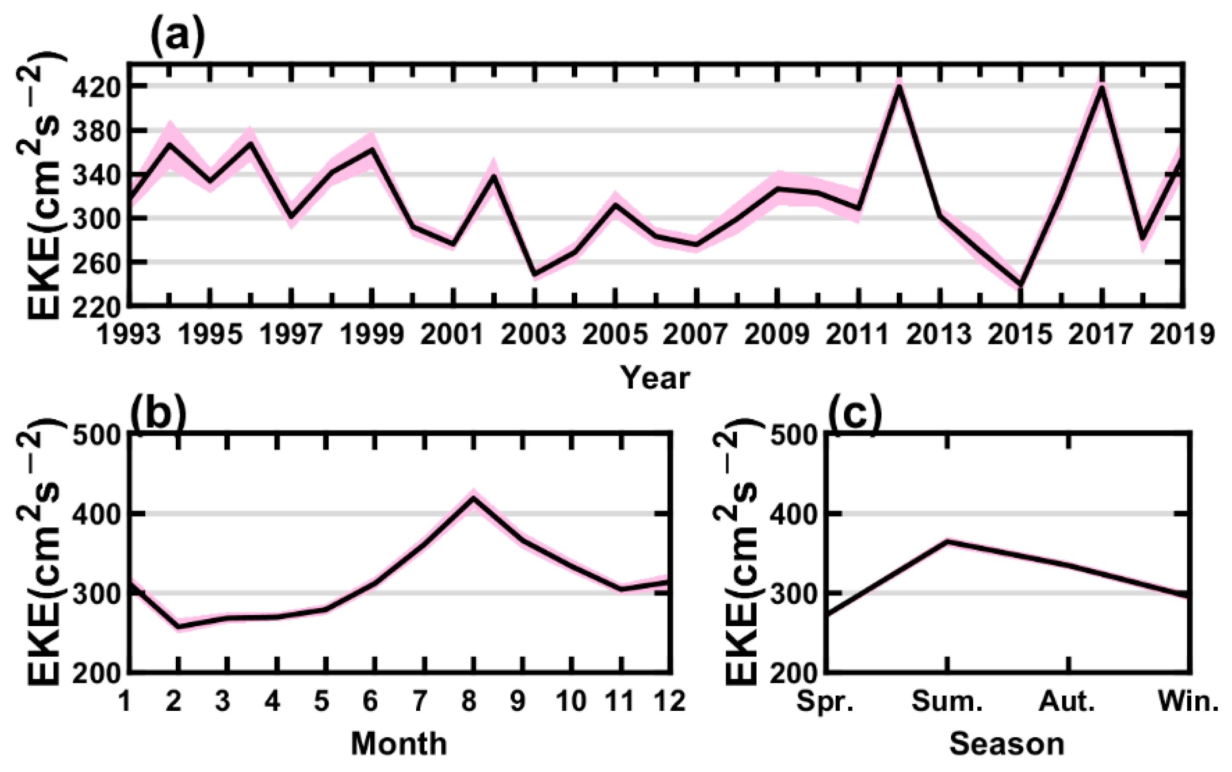
3.1.3. Temporal Variations of Anticyclonic Eddy Kinetic Energy

Figure 7 shows the variations in anticyclonic eddy kinetic energy (AEKE). The annual mean AEKE is ~316.7 cm2 s−2 on average. In 2012, the annual mean AEKE was the largest (~419.4 cm2 s−2). While the annual mean AEKE in 2017 (~418.3 cm2 s−2) was only next to that in 2012. The minimum annual mean AEKE appeared in 2015, and the second in 2003, with the AEKE being only ~239.0 cm2 s−2 and ~249.0 cm2 s−2, respectively. From 1993 to 2003, the annual mean AEKE tended to decrease. In 1993 and 1994, the annual mean AEKE values were ~316.9 cm2 s−2 and ~366.6 cm2 s−2, respectively. Then the annual mean AEKE decreased to ~249.0 cm2 s−2 in 2003. After 2003, the AEKE gradually increased to ~419.4 cm2 s−2 in 2012, which was the maximum annual mean AEKE. From 2013 to 2019, there was a large fluctuation in the annual mean AEKE.
The variation in monthly mean AEKE is similar to that of the anticyclonic eddy number. The difference between them is that the maximum monthly mean anticyclonic eddy number appears in May (Figure 5b), but the monthly mean AEKE is largest in August. From February to May, the monthly mean AEKE barely increases. In February, the monthly mean AEKE is ~257.3 cm2 s−2, which is the minimum monthly mean AEKE. Then the monthly mean AEKE gradually increases to ~278.9 cm2 s−2 in May, with an increase of ~2.7% per month only. After May, the increasing rate of monthly mean AEKE is much larger (~14.5% per month from May to August), and the monthly mean AEKE reaches its maximum (~418.6 cm2 s−2) in August. After August, the monthly mean AEKE decreases sharply to ~304.3 cm2 s−2 in November.
The seasonal variation of AEKE is clear (Figure 7c). In spring, the AEKE is ~272.3 cm2 s−2, which is the smallest among the four seasons. In summer, the AEKE increases sharply to the maximum of ~364.3 cm2 s−2. Then the AEKE gradually decreases to ~334.4 cm2 s−2 and ~295.5 cm2 s−2 in autumn and winter, respectively.

3.1.4. Temporal Variations of Anticyclonic Eddy Amplitude

From 1993 to 2009, the minimum annual mean eddy amplitude was ~5.8 cm while the maximum one was ~6.7 cm (Figure 8a), indicating that the variation of annual mean eddy amplitude was not large during this period. But it is still obvious that the eddy amplitude tended to decrease during 1993–2003. From 2003 to 2012, the annual mean eddy amplitude increased from ~5.8 cm (in 2003) to ~7.2 cm (in 2012). After 2013, the minimum anticyclonic eddy amplitude appeared in 2015 (~5.6 cm) and the maximum appeared in 2017 (~7.5 cm). As for the variation of monthly mean eddy amplitude (Figure 8b), there exists a maximum in August (~6.7 cm), while the minimum appears in February (~5.3 cm). The monthly mean eddy amplitude increases from February, reaching the maximum in August, and then decreases gradually to November. The seasonal mean eddy amplitude ranges from ~6.1 cm to ~6.5 cm, with the peak appearing in summer. The statistical difference of the eddy amplitude in different years (months/seasons) is not as evident as the other characteristics mentioned above, but the variation trend is similar to that of other characteristics.

3.1.5. Temporal Variations of Total Area of Anticyclonic Eddy

The total area of anticyclonic eddies (TAAE) in the SCS is about 2.24 × 10⁵ km2 on average, accounting for about 11.5% of the whole SCS area (only the area deeper than 100 m is considered). From 1993 to 2019, the maximum annual mean TAAE appeared in 2012, with a total area of ~2.59 × 10⁵ km2, second in 1994, about 2.49 × 10⁵ km2 (Figure 9a). The minimum annual mean TAAE was about 1.97 × 10⁵ km2 in 2019, and about 2.00 × 10⁵ km2 in 2006. As for the inter-annual variation, from 1993 to 2003, the annual mean TAAE decreased gradually. After 2004, though there were fluctuations, the annual mean TAAE also showed a tendency to increase in general. The annual mean TAAE reached its maximum in 2012 and then decreased sharply to 2015. After 2013, the same with the annual mean AEKE and eddy amplitude, the minimum and maximum annual mean TAAE appeared in 2015 and 2017, respectively.
The variation in the monthly (seasonal) mean TAAE is about the same as that of monthly (seasonal) mean AEKE (Figure 9b,c): the monthly mean TAAE increases from January, reaching the maximum in August (~2.71 × 10⁵ km2), and then gradually decreases to the minimum in December (~1.77 × 10⁵ km2). Similarly, the seasonal mean TAAE increases from spring (~2.33 × 10⁵ km2), reaching the maximum in summer (~2.58 × 10⁵ km2), and then decreases to the minimum in winter (~1.93 × 10⁵ km2).

3.2. Spatial Distributions of Anticyclonic Eddy Characteristics in the SCS

3.2.1. Spatial Distributions of Anticyclonic Eddy Number and Anticyclonic Eddy Frequency

Spatial distributions of anticyclonic eddy number and anticyclonic eddy frequency during 1993–2019 are shown in Figure 8. In the SCS, anticyclonic eddies occurred most frequently in the area centered at 112°E, 9.5°N, with a radius of about 58 km (Circle A1 in Figure 10b). This area was occupied by about 160 anticyclonic eddies in total, accounting for ~40% of the time from 1993 to 2019 (Figure 10b). The area centered at 113.4°E, 17.1°N, with a radius of about 50 km, is the other area where anticyclonic eddies were active (Circle A2 in Figure 10b). This area was occupied by anticyclonic eddies about 25% of the time, and about 144 anticyclonic eddies occurred there during 1993–2019. In general, the anticyclonic eddy is active in the central SCS (the area with a depth deeper than 2000 m).
No matter the season, the anticyclonic eddies are active in the area near 2000 m isobaths (especially the area north of 15°N), with the eddy frequency higher than 20%. In spring, the anticyclonic eddies occur most frequently in the areas such as Circle A1, southwest of Taiwan Island and west of Luzon Island. As for summer, the anticyclonic eddies are not so active in the west of Luzon Island, while the eddy is still active in the southwest of Taiwan Island and the areas within Circles A1 and A2. Meanwhile, the anticyclonic eddies are also active in the southwestern SCS in summer, which may be influenced by the “Nansha upper anticyclone” [38]. The eddy frequency is statistically lower in autumn than in other seasons, with a maximum frequency of less than 30% in the SCS. But the eddy frequency in the area deeper than 2000 m is still much higher than that in other areas. In winter, the anticyclonic eddies are active again in the west of Luzon Island (with eddy frequency higher than 30%), the area east of Vietnam and the area southwest of Luzon Island.

3.2.2. Spatial Distributions and Variations of Anticyclonic Eddy Lifetime

Figure 11 shows the mean eddy lifetime corresponding to their generation place. The general mean eddy lifetime is not long, so only a few eddies have a lifetime longer than (or equal to) 60 days. Eddies generated in the central basin of SCS (especially eddies generated in the mid-latitudes, i.e., 13°–17°N) have a longer lifetime (Figure 11b), as they would have a longer distance to propagate. In spring and summer, eddies generated in the northeast of Vietnam have a longer lifetime. But actually, only three eddies were generated in spring there from 1993 to 2019, with an eddy lifetime of 113, 78 and 105 days, respectively (generated on 1 May 1998, 23 April 2000 and 26 May 2003, respectively). As for autumn and winter, eddies generated in the deep basin still have a longer lifetime.

3.2.3. Spatial Distributions and Variations of AEKE

Figure 12 shows the distributions of climatological mean and seasonal mean AEKE in the SCS during 1993–2019. The AEKE in the SCS ranges between ~49.3 cm2 s−2 and ~1004.0 cm2 s−2 (Figure 12a). The area east of Vietnam (Box B1 in Figure 12a) and the area southwest of Taiwan Island (Box B2 in Figure 11a) are two areas where the AEKE is significantly larger than that in other areas, with the AEKE being more than 1000 cm2 s−2.
The zonal mean AEKE is largest in 21–22°N (Figure 12b), corresponding to the high AEKE in the southwest of Taiwan Island. To the south of 20 °N, the zonal mean AEKE is largest at 12 °N, where the AEKE is extraordinarily high in the east of Vietnam (Figure 12a,b). Except for areas B1 and B2, the AEKE is less than 500 cm2 s−2 in other areas of the SCS. In terms of the anticyclonic eddy frequency (Figure 10b) or the magnitude of AEKE, Box B1 (109.5°–113.5°E, 9°–15.5°N) is the area where anticyclonic eddies are most active in the SCS. In the south part and west part of Box B1, the AEKE can reach a magnitude of more than 1000 cm2 s−2. In the northeast part of Box B1, the AEKE is relatively smaller, but the AEKE is still more than 500 cm2 s−2. Box B2 (118.5°–121°E, 20°–21.5°N) is much smaller than Box B1, in terms of the area. The magnitude of AEKE in Box B2 is equal to or even more than that in Box B1. The AEKE in Box B3 (see Figure 12a) is smaller than in Box B1 or Box B2, but larger than that in most other areas in the SCS (Figure 12a), with the AEKE between 400 cm2 s−2 and 600 cm2 s−2.
In spring, the AEKE is large in Box B2, Box B3 and the middle and north parts of Box B1, with the AEKE reaching 600–800 cm2 s−2 (Figure 10c). As a contrast, the AEKE in other areas is about 200 cm2 s−2 or even less. In summer, the AEKE in Box B1 has a great increase (Figure 10d), with the largest AEKE being more than 1100 cm2 s−2. The AEKE in Box B2 is also large in summer while the AEKE in Box B3 is small. In autumn, the south part of Box B1 is the area where the AEKE is the largest in the whole SCS, with its magnitude ranging from 800 to 1000 cm2 s−2 (Figure 10e). In Box B2, the range with high AEKE (i.e., AEKE higher than 600 cm2 s−2) almost covers the whole Box B2. In winter, the large AEKE in Box B1 disappears, with spatial-averaged AEKE of about 200 cm2 s−2 (Figure 10f). But the AEKE in Box B2 sharply increases, reaching the maximum of the whole area in the SCS all year around, with the AEKE of more than 1200 cm2 s−2 in almost the whole Box B2 and up to ~1584.5 cm2 s−2. Box B3 is also influenced by the extraordinarily high AEKE, resulting in high AEKE (600 cm2 s−2 or more) in the northeast part of Box B3.

3.2.4. Spatial Distributions and Variations of Anticyclonic Eddy Amplitude

It is evident that the anticyclonic eddy amplitude in the northern SCS is larger than that in the southern SCS, especially in Spring. As shown in Figure 13a, the anticyclonic eddy amplitude in the area south of 13°N (except the area with a depth deeper than 2000 m) is smaller than that in the northern SCS, with an amplitude of no more than 6.0 cm on average. Areas with a high AEKE are also where the eddy amplitude is large (e.g., the southern part of Box B1 and Box B2 in Figure 12a). In the SCS, the anticyclonic eddy amplitude decreases with the latitude decreasing (Figure 13b). Only in the area north of 20°N, the anticyclonic eddy amplitude would be larger than 10 cm on average. The eddy amplitude is largest in the southeast of Vietnam (in summer) and southwest of Taiwan Island (in winter). In spring, the eddy amplitude is large in the northern part of SCS, especially near the Luzon Strait. In summer, the eddy amplitude is largest in the east of Vietnam, exactly the Box B1 in Figure 12a. The eddy amplitude in the southeast of Vietnam remains large in autumn but becomes small in winter. The amplitude in the southwest of Taiwan Island is large all year around, but it is extremely large in winter. The eddy amplitude in the southwest of Taiwan Island can reach more than 20 cm in winter, which is the largest in the whole SCS all year around. To the north of 13°N in the SCS, the eddy amplitude is smaller in winter than in other seasons, except the southwest of Taiwan Island and west of Luzon Island (Figure 13c–f).

3.2.5. Spatial Distributions and Variations of Anticyclonic Eddy Radius

The eddy radius is chosen to represent the eddy area in the following analyses. The Rossby radius of deformation is often associated with the eddy size, and it is influenced by the depth, buoyancy frequency and the Coriolis parameter f [5]. Figure 14c shows the Rossby radius of deformation estimated from WOA2018. As the latitude decreases, the Rossby radius of deformation increases in the SCS, resulting in the increase of the eddy radius (Figure 14b). From about 23°N to 15°N, the eddy radius increases from ~74.9 km to ~86.3 km and then varies around 86.0 km in 6°–14°N. In the northeastern SCS, the eddy radius is relatively smaller than in the central basin and western or southern SCS. Similar to other characteristics (e.g., AEKE, eddy amplitude and eddy frequency), the eddy radius in the southeast of Vietnam is larger than that in any other areas in summer and autumn (Figure 14d,e). As a result, the climatological mean eddy radius there is also large (Figure 14a). In winter, the eddy radius is large in the southern SCS, which may be influenced by the anticyclonic current there in winter [1,39,40], and such a large-scale current would drive the generation of anticyclonic eddies with a large radius.

4. Discussion

4.1. The Anticyclonic Eddy Number

In this study, the shortest eddy lifetime is limited to 10 days, so the eddy number is much more than that in previous studies. To make a comparison with previous studies, the number of eddies whose lifetime is more than 30 days (called long-term eddies in this study) is shown in Figure 15. The annual mean long-term eddy number had a decreasing tendency from 1993 to 2003. In 2003–2006, the long-term eddy number fluctuated greatly. After 2006, the annual mean long-term eddy number had an increasing tendency from 2006 to 2014, and then the annual mean long-term eddy number fluctuated around 45. The monthly mean long-term eddy number has a similar variation tendency with the total eddy number (Figure 5b and Figure 15b), but the maximum appears in July (Figure 15b). The seasonal variation in the long-term eddy number is different from that of the total one, as the seasonal mean long-term eddy number increases from spring, reaching the maximum in summer, and then decreasing to a minimum in the winter. This is similar to the seasonal variations of other characteristics (e.g., AEKE, eddy amplitude).
Previous studies had different opinions about the variations of anticyclonic eddy numbers in the SCS. Wang et al. [3] calculated the eddy number in the SCS, showing that anticyclonic eddies were most active from April to June during 1993–2000. The results (time range: October 1993 to October 2009) of Chen et al. [5] showed that from March to September, the anticyclonic eddy number is significantly larger than in other months. Using the merged data provided by the AVISO, Lin et al. [41] showed a variation tendency similar to this study (time range: 1993–2009), with the eddy number maximum appearing in July (the anticyclonic eddy number in June or August is slightly fewer than that in July). Feng et al. [42] tracked the eddies in the SCS by satellite data and model data, respectively, finding that the number of anticyclonic eddies in late spring or summer is much larger than that in autumn or winter. In general, the anticyclonic eddies in the SCS are active from about March to about September (Figure 5b and Figure 15b). Previous studies showed that the maximum anticyclonic eddy number appears in July–September, while the anticyclonic eddy number is obviously larger in May in this study (Figure 5b). The eddies whose lifetime is less than 30 days (called short-term eddy in this study) account for about 78% (Figure 15d) of all detected anticyclonic eddies while these eddies were ignored in previous studies. When these anticyclonic eddies are removed from the statistics, as the monthly mean long-term eddy number mentioned before, the maximum monthly mean anticyclonic eddy number appears in July (Figure 15b), and the eddy numbers in May–August are apparently larger than that in other months. This indicates that the eddies whose lifetime is longer than 30 days are active in May–August, and there are much more short-term eddies in May. The SCS is an area influenced significantly by the monsoon, and the wind stress curl plays an important role in the generation of eddies [14]. May is exactly the monsoon transition season. Whether such amounts of short-term eddies are active in May is related to the transition of monsoon or not still needs further investigation.

4.2. Variation of AEKE

4.2.1. Sharp Increase of AEKE in Summer

The AEKE in the east of Vietnam is about 600 cm2 s−2 in the spring and then increases to more than 1000 cm2 s−2 in the summer (Figure 12b). Such a strong AEKE covers a wide range and lasts for a long time. Until autumn, the seasonal mean AEKE there is still more than 800 cm2 s−2 (Figure 12c). This may be due to the following reasons. First, previous studies showed that eddies in Box B1 are more active in summer [37,43,44,45], especially in August. These eddies are mainly generated in June or early July, reaching their mature stage in August. Second, the eddy activities are strongly influenced by wind [46,47]. Previous studies showed that wind stress curl is an important factor driving the generation of eddy east of Vietnam. During the summer, when the southwest monsoon prevails, the wind stress curl would drive the generation of a strong eddy dipole [48], resulting in a large AEKE there. The eddy dipole survives for a long time, until October or even November, so the AEKE is still large in autumn. Finally, the eddy kinetic energy is related to the baroclinic instability of the ocean current, especially the boundary current [49,50]. In the east of Vietnam, there is a strong western boundary current (namely “Vietnam offshore current”) [51]. The western boundary current provides negative vorticity to the anticyclonic eddies, making the anticyclonic eddies active in summer with a large AEKE. Following Sun et al. [52], we calculate the areal integral of positive (PWSC) and negative (NWSC) parts of wind stress curl in the same area of 109.5°–113.5°E and 9°–13°N (Box E2 in Figure 1). It can be seen from Figure 16 that low NWSC values beyond the standard deviation (values plotted in red) occur most in the summer. Following Liang [53], we calculate the information flow from the NWSC to the AEKE in the same area using the following equation:
T 2 1 = C 11 C 12 C 2 , d 1 C 12 2 C 1 , d 1 C 11 2 C 22 C 11 C 12 2
where the C i j is the sample covariance between time series X i and X j , and C i ,   d j is the sample covariance between X i and X ˙ j ( X ˙ j = d X j ( n ) d t = X j ( ( n + 1 ) X j ( n ) t ). Information flow T 2 1 > 0 indicates that X 2 is one of the causes of X 1 , otherwise X 2 is irrelevant to X 2 . The results (Table 1) show that only in spring and summer, the values of information flow from NWSC to AEKE are positive, with a relatively larger value in the summer (0.0013 only). Though the value is small, it still indicates that the wind stress curl has a relatively stronger impact on the AEKE in summer rather than in other seasons. Such a small value implies that wind stress curl may have an indirect influence on the AEKE. This is consistent with Cheng et al. [37]: at first, the wind stress curl determines the strength of the upper-layer large-scale circulation to a large extent, and then barotropic/baroclinic instability (mainly baroclinic instability) of the mean flow converts mean kinetic energy/available potential energy to EKE.

4.2.2. AEKE Maximum in the Southwest of Taiwan Island

In the southwest of Taiwan Island, i.e., Box B2 in Figure 12a, the AEKE in spring, summer or autumn fluctuates around 600.0 cm2 s−2. While in winter, the AEKE in Box B2 increases to more than 1000.0 cm2 s−2, with the largest value of 1584.5 cm2 s−2. The area southwest of Taiwan Island, or the west of Luzon Strait (Box B2), is the main zone for the Kuroshio intrusion [1,40,54,55]. In this area, the Kuroshio would intrude by way of a current “ring” or a current “loop”, reaching as far as 117°E [56,57]. The Kuroshio intrusion is largely influenced by the monsoon and has a significant seasonal variation [58,59,60]. In the winter, the Kuroshio mainly intrudes in the SCS by a “direct branch” or an “anticyclonic ring” [1,60], resulting in rich “anticyclonic eddies shedding” events west of Luzon Strait [58]. Figure 17 presents the Double-Index from 1993 to 2019, calculated by using the method of Huang et al. [61]:
K W I = s i g n V g V g d A
K C I = s i g n V g V g d A
where s i g n x is the sign function (when x 0 , s i g n x = 1 , when x < 0 , s i g n x = 0 ), V g is the relative vorticity of surface geostrophic currents, and A is the integrated area (Box E1 in Figure 1). The low values beyond the standard deviation (values shaded in red) appear mostly in winter. Such a negative value of KWI indicates a remarkable Kuroshio current loop in the Luzon Strait, resulting in prolonged anticyclonic eddies southwest of Taiwan Island. We also examine the information flow from the KWI to the AEKE in the corresponding area (Box E1 in Figure 1, Table 1). As revealed by the information flow, the Kuroshio intrusion is not the factor influencing the AEKE in summer, while the information flow is positive in the spring (0.0027), autumn (0.0237) and winter (0.2069), indicating that the Kuroshio intrusion has a relative weaker impact but a strong influence on the AEKE there in spring (autumn) and winter, respectively. Furthermore, the climatological mean SST also shows that Kuroshio intrusion is more active in the winter. This is why the AEKE in Box B2 would strengthen significantly in winter. On one hand, because of the Kuroshio intrusion, there are lots of eddies shedding from the Kuroshio or propagating from the Northwest Pacific, leading to the active anticyclonic eddies; on the other hand, the intrusion of Kuroshio provides enough energy for the activities of anticyclonic eddies.

4.3. Temporal Variations of Anticyclonic Eddy Characteristics

4.3.1. General Variation Trends of Annual Mean Anticyclonic Eddy Characteristics in the SCS

Figure 18a shows the variations of the five selected annual mean parameters of long-term anticyclonic eddies after normalization. These five parameters had a similar variation trend from 1993 to 2019. Before 2013, the variations in these five parameters had a transition in 2004, 2005 or 2006. From 1993 to 2004–2006, these five parameters had a decreasing trend. After 2004–2006, these five parameters had an increasing trend until around 2012. From 2012, they decreased at first, and then increased again, with the minimum appearing in 2015 and the maximum appearing in 2017. The variation feature can be also captured by the characteristics of all anticyclonic eddies (see Figure 5, Figure 6, Figure 7, Figure 8 and Figure 9).
A previous study has already shown the impact of El Niño–Southern Oscillation (ENSO) and the Pacific meridional modes (PMMs) on the eddy in the SCS [62]. The inter-annual variation of wind stress curl in the SCS is related to the ENSO and PMMs, leading to the inter-annual variation of eddy number. Tuo et al. [62] made a summary that before 2004 (from 1993 to 2003), ENSO strongly impacted the eddy number in the SCS through the additive effects of both ENSO and PMMs, but it had little impact on the SCS eddy after 2004. In this study, the variation tendency of the five parameters had a transition in 2004–2006. Here, we conduct the same analysis with Tuo et al. [62] and the results are shown in Figure 18b (blue line). As the inter-annual variation is what we are concerned about, an 11-month running mean has been applied to the eddy number and the Niño-3.4 index. Figure 18b shows the sliding correlation coefficient between the eddy number and Niño-3.4 index using a 10-year moving window. As with Tuo et al. [62], the relationship changed around 2004 from relatively significant and negatively correlated before to noncorrelated afterward. The coefficients between Niño-3.4 index and other characteristics show a similar transition around 2004. We also calculate the information flow from ENSO to the eddy number using the same moving window, showing a similar transition in 2004–2006 (red line in Figure 18b), but with a low value pre-2004. Indeed, as revealed by the correlation and the information flow, ENSO had a relatively strong impact on the anticyclonic eddies in the 10-year window of 1999–2008 (the value is relatively higher in 2004–2006). The effects of ENSO and PMMs may be the mechanisms of the inter-annual variation of these parameters, but it still needs further study to confirm the effects of ENSO and PMMs on the annual variation of these characteristics of anticyclonic eddies.

4.3.2. Monthly Variations of Anticyclonic Eddy Characteristics

It can be seen that the anticyclonic eddies are more active in summer and relatively passive in winter. As discussed above, the wind has an important impact on the eddy activities. The negative wind stress curl (WSC) was deemed to favor the activities of anticyclonic eddies. Though the monthly mean WSC in the SCS is relatively lower in summer, it is only negative in June (red line in Figure 19). It seems that the WSC in the whole year does not benefit the anticyclonic eddy activities. The black line in Figure 19 shows that from April to September, as the southwest monsoon prevails, the area with negative WSC occupies more than 50% of the SCS. The variation in the percentage (black line in Figure 19) is highly correlated with the monthly variations of some characteristics of anticyclonic eddies. Such a high percentage indicates that in the boreal summer year, there are more areas favoring the activities of anticyclonic eddies. The WSC indeed influences the anticyclonic eddies, and there may be other factors that have a considerable impact on the anticyclonic eddies due to the relatively lower monthly mean WSC.

5. Conclusions

Anticyclonic eddies are important for high phytoplankton biomass and high primary production at their edges. Previous studies focused on the long-term eddies and tended to discuss anticyclonic eddies and cyclonic eddies together in the SCS. The characteristics of short-term anticyclonic eddies were ignored. As the daily ADT data are available now, this study limits the shortest lifetime to 10 days, so that the short-term eddies can be also taken into account. The characteristics of anticyclonic eddies in the SCS are studied more comprehensively. We use the TPI parameter to represent the local anomaly of ADT and then map the anticyclonic eddies in the SCS. The TPI parameter is easy to calculate and to distinguish anticyclonic eddy and cyclonic eddy. In this study, we mainly focus on the five characteristics of anticyclonic eddies, specifically anticyclonic eddy number (or anticyclonic eddy frequency), anticyclonic eddy lifetime, anticyclonic eddy kinetic energy, anticyclonic eddy amplitude and anticyclonic eddy area (or radius). The key conclusions of this study are:
(1)
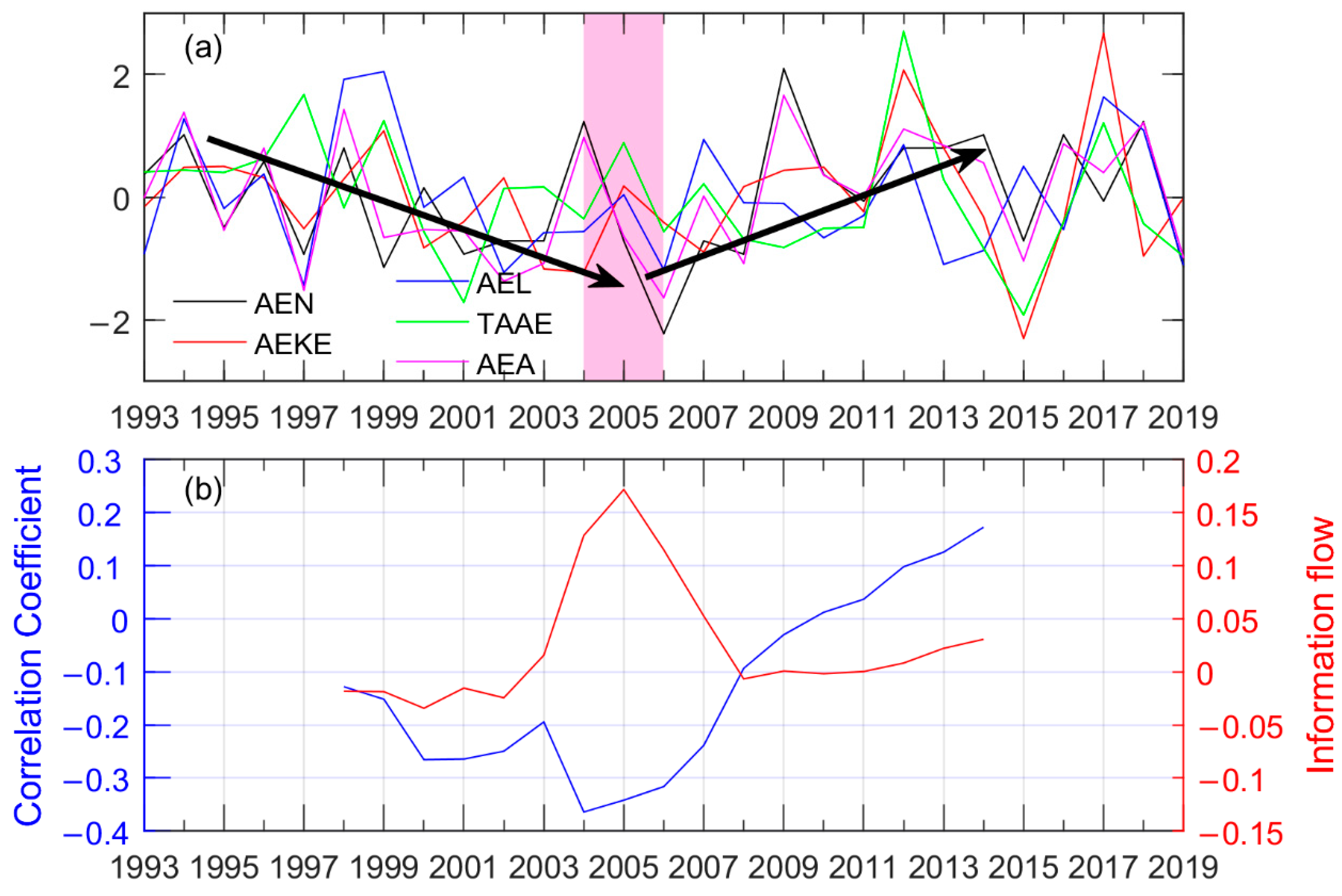
The five selected parameters of anticyclonic eddies have similar interannual variation trends, especially during the time from 1993 to 2012. From 1993 to ~2004, these five parameters gradually decreased, and then increased to a maximum in 2012; after 2013, the variation trend is not so clear, though the minimums of most of these parameters appeared in 2015 and the maximums appeared in 2017. As revealed by the correlation coefficient and information flow, the ENSO may be the reason for the transition of the annual variation, and the ENSO had a relatively stronger impact on the variation during 1999–2008.
(2)
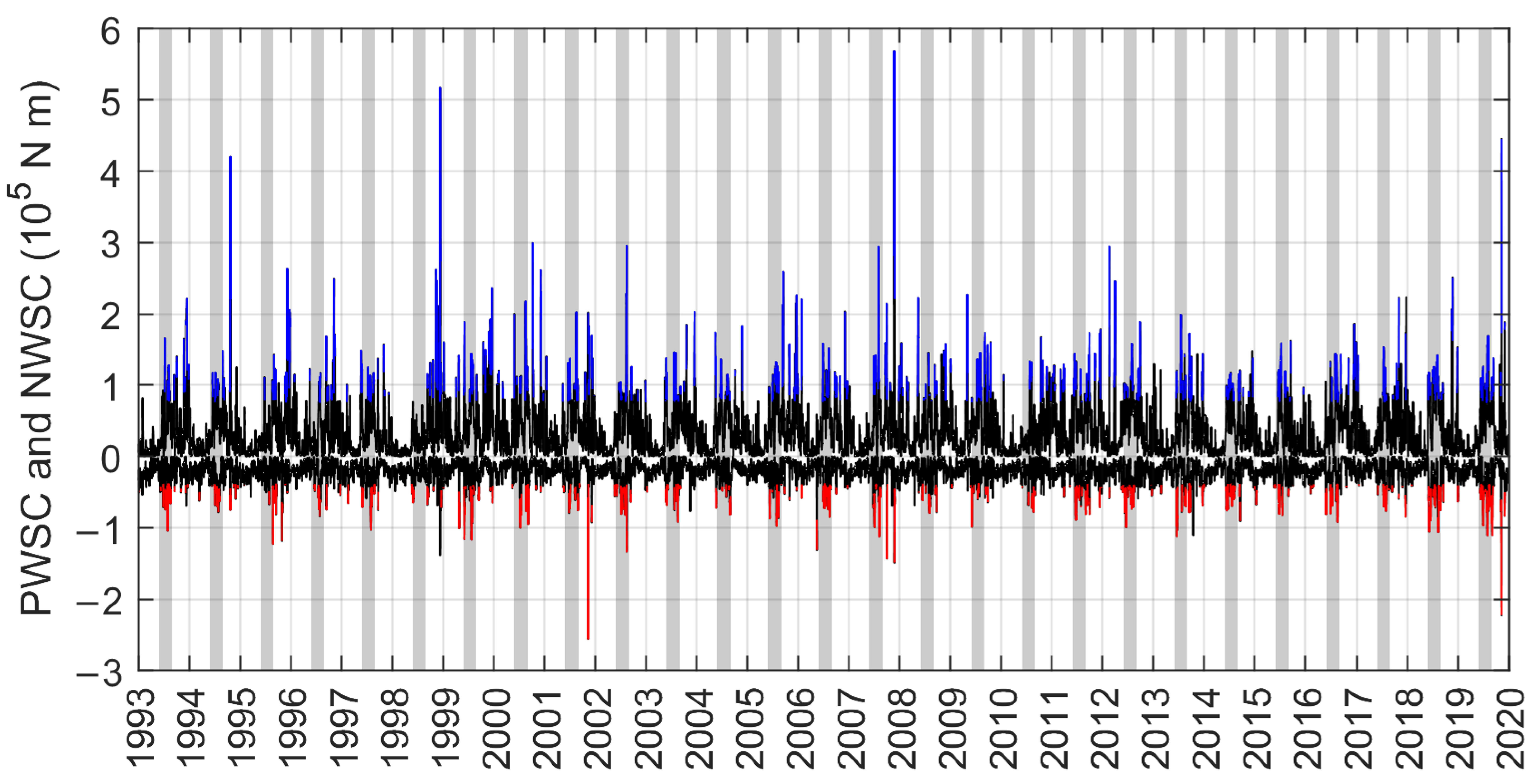
The wind may be a key factor that influences the anticyclonic eddies in the SCS. For the monthly variation, as the southwest monsoon prevails, the percentage of area with negative WSC occupies more than 50% of the SCS, resulting in active eddy activity in the boreal summer year (from March to September). For the spatial distribution, the combining effects of wind stress curl and western boundary currents (e.g., Vietnam offshore current and Kuroshio) may be the main mechanisms of the large eddy frequency and large AEKE in the east of Vietnam and southwest of Taiwan Island.
(3)
Anticyclonic eddies are more active in the area deeper than 2000 m, with higher eddy amplitude, AEKE and other characteristics. In spring, summer and autumn, anticyclonic eddies are active in the east of Vietnam (Box B1 in Figure 12a), the southwest of Taiwan Island (Box B2 in Figure 12a) and the areas near the 2000 m isobaths. In the winter, the west of Luzon Island is the area where the anticyclonic eddies are relatively active, in terms of relatively higher eddy frequency, AEKE and anticyclonic eddy amplitude.
It should be noted that there are still some abnormal eddies in the SCS that cannot be detected by our method. The eddies that have negatively correlated SSH–SST relationships [63,64] may also play an important role in ocean dynamics and biogeochemical activities. These eddies are also found in the SCS [35,36], though with low frequency. As a census study, we do not remove these abnormal eddies. How these eddies influence the basic features of anticyclonic eddies in the SCS needs further research. The method would be improved by taking the sea surface temperature data into account. This would be the key point of our future work.

Author Contributions

Conceptualization, J.H. and W.S.; funding, J.H.; methodology, W.S. and J.H.; writing—original draft preparation, W.S.; writing—review and editing, W.S. and J.H. All authors have read and agreed to the published version of the manuscript.

Funding

This study was jointly supported by the National Natural Science Foundation of China (91958203, 41776027 and 41730533).

Data Availability Statement

The datasets for the research are publicly available. The ADT data are provided by Copernicus Marine Environment Monitoring Service (CMEMS) via https://data.marine.copernicus.eu/product/SEALEVEL_GLO_PHY_L4_MY_008_047/description (accessed on 10 August 2022). The wind data are provided by National Centers for Environmental Information, NOAA via https://www.ncdc.noaa.gov/data-access/model-data/model-datasets/climate-forecast-system-version2-cfsv2 (accessed on 9 September 2022). The ocean Niño Index is obtained directly from National Oceanic and Atmospheric Administration (NOAA) via https://origin.cpc.ncep.noaa.gov/products/analysis_monitoring/ensostuff/ONI_v5.php (accessed on 15 September 2022).

Acknowledgments

We appreciate all the constructive comments from the Editor and anonymous reviewers that have improved early version of the manuscript.

Conflicts of Interest

The authors declare no conflict of interest. The funders had no role in the design of the study; in the collection, analyses, or interpretation of data; in the writing of the manuscript, or in the decision to publish the results.

References

  1. Hu, J.Y.; Kawamura, H.; Hong, H.S.; Qi, Y.Q. A review on the currents in the South China Sea: Seasonal circulation, South China Sea warm current and Kuroshio intrusion. J. Oceanogr. 2000, 56, 607–624. [Google Scholar] [CrossRef]
  2. Zheng, Q.A.; Xie, L.L.; Zheng, Z.W.; Hu, J.Y. Progress in research of mesoscale eddies in the South China Sea. Adv. Mar. Sci. 2017, 35, 131–158. [Google Scholar] [CrossRef]
  3. Wang, G.H.; Su, J.L.; Chu, P.C. Mesoscale eddies in the South China Sea observed with altimeter data. Geophys. Res. Lett. 2003, 30, 2121. [Google Scholar] [CrossRef]
  4. Liu, Q.Y.; Kaneko, A.; Su, J.L. Recent progress in studies of the South China Sea circulation. J. Oceanogr. 2008, 64, 753–762. [Google Scholar] [CrossRef]
  5. Chen, G.X.; Hou, Y.J.; Chu, X.Q. Mesoscale eddies in the South China Sea: Mean properties, spatiotemporal variability, and impact on thermohaline structure. J. Geophys. Res. Oceans 2011, 116, C06018. [Google Scholar] [CrossRef]
  6. Chelton, D.B.; Schlax, M.G.; Samelson, R.M.; de Szoeke, R.A. Global observations of large oceanic eddies. Geophys. Res. Lett. 2007, 34, 87–101. [Google Scholar] [CrossRef]
  7. Chelton, D.B.; Schlax, M.G.; Samelson, R.M. Global observations of nonlinear mesoscale eddies. Prog. Oceanogr. 2011, 91, 167–216. [Google Scholar] [CrossRef]
  8. Mason, E.; Pascual, A.; McWilliams, J.C. A new sea surface height–based code for oceanic mesoscale eddy tracking. J. Atmos. Ocean. Technol. 2014, 31, 1181–1188. [Google Scholar] [CrossRef]
  9. Faghmous, J.H.; Frenger, I.; Yao, Y.S.; Warmka, R.; Lindell, A.; Kumar, V. A daily global mesoscale ocean eddy dataset from satellite altimetry. Sci. Data 2015, 2, 150028. [Google Scholar] [CrossRef]
  10. Nencioli, F.; Dong, C.M.; Dickey, T.; Washburn, L.; McWilliams, J.C. A vector geometry–based eddy detection algorithm and its application to a high-resolution numerical model product and high-frequency radar surface velocities in the Southern California Bight. J. Atmos. Ocean. Technol. 2010, 27, 564–579. [Google Scholar] [CrossRef]
  11. Sadarjoen, I.A.; Post, F.H. Detection, quantification, and tracking of vortices using streamline geometry. Comput. Graph. 2000, 24, 333–341. [Google Scholar] [CrossRef]
  12. Xu, G.J.; Cheng, C.; Yang, W.X.; Xie, W.H.; Kong, L.M.; Hang, R.L.; Ma, F.; Dong, C.M.; Yang, J.S. Oceanic eddy identification using an AI scheme. Remote Sens. 2019, 11, 1349. [Google Scholar] [CrossRef]
  13. Lin, P.F.; Wang, F.; Chen, Y.L.; Tang, X.H. Temporal and spatial variation characteristics on eddies in the South China Sea I. Statistical analyses. Acta Oceanol. Sin. 2007, 29, 14–22. [Google Scholar] [CrossRef]
  14. Xiu, P.; Chai, F.; Shi, L.; Xue, H.J.; Chao, Y. A census of eddy activities in the South China Sea during 1993–2007. J. Geophys. Res. Oceans 2010, 115, C03012. [Google Scholar] [CrossRef]
  15. Du, Y.Y.; Yi, J.W.; Wu, D.; He, Z.G.; Wang, D.X.; Liang, F.Y. Mesoscale oceanic eddies in the South China Sea from 1992 to 2012: Evolution processes and statistical analysis. Acta Oceanol. Sin. 2014, 33, 36–47. [Google Scholar] [CrossRef]
  16. He, Q.Y.; Zhan, H.G.; Cai, S.Q.; He, Y.H.; Huang, G.L.; Zhan, W.K. A new assessment of mesoscale eddies in the South China Sea: Surface features, three-dimensional structures, and thermohaline transports. J. Geophys. Res. Oceans 2018, 123, 4906–4929. [Google Scholar] [CrossRef]
  17. McGillicuddy, D.J., Jr.; Robinson, A.R. Eddy-induced nutrient supply and new production in the Sargasso Sea. Deep-Sea Res. I Oceanogr. Res. Pap. 1997, 44, 1427–1450. [Google Scholar] [CrossRef]
  18. Vaillancourt, R.D.; Marra, J.; Seki, M.P.; Parsons, M.L.; Bidigare, R.R. Impact of a cyclonic eddy on phytoplankton community structure and photosynthetic competency in the subtropical North Pacific Ocean. Deep-Sea Res. I Oceanogr. Res. Pap. 2003, 50, 829–847. [Google Scholar] [CrossRef]
  19. Wang, L.; Huang, B.Q.; Laws, E.A.; Zhou, K.B.; Liu, X.; Xie, Y.Y.; Dai, M.H. Anticyclonic eddy edge effects on phytoplankton communities and particle export in the northern South China Sea. J. Geophys. Res. Oceans 2018, 123, 7632–7650. [Google Scholar] [CrossRef]
  20. Jing, Z.Y.; Qi, Y.Q.; Fox-Kemper, B.; Du, Y.; Lian, S.M. Seasonal thermal fronts on the northern South China Sea shelf: Satellite measurements and three repeated field surveys. J. Geophys. Res. Oceans 2016, 121, 1914–1930. [Google Scholar] [CrossRef]
  21. Weiss, A.D. Topographic Position and Landforms Analysis. In Proceedings of the ESRI International User Conference, San Diego, CA, USA, 9–13 July 2001. [Google Scholar]
  22. Huang, Z.; Feng, M. Remotely sensed spatial and temporal variability of the Leeuwin Current using MODIS data. Remote Sens. Environ. 2015, 166, 214–232. [Google Scholar] [CrossRef]
  23. Xie, S.Y.; Huang, Z.; Wang, X.H.; Leplastrier, A. Quantitative Mapping of the East Australian Current Encroachment Using Time Series Himawari-8 Sea Surface Temperature Data. J. Geophys. Res. Oceans 2020, 125, e2019JC015647. [Google Scholar] [CrossRef]
  24. Huang, Z.; Wang, X.H. Mapping the spatial and temporal variability of the upwelling systems of the Australian south-eastern coast using 14-year of MODIS data. Remote Sens. Environ. 2019, 227, 90–109. [Google Scholar] [CrossRef]
  25. Huang, Z.; Hu, J.Y.; Shi, W.A. Mapping the coastal upwelling east of Taiwan using geostationary satellite data. Remote Sens. 2021, 13, 170. [Google Scholar] [CrossRef]
  26. Shi, W.A.; Huang, Z.; Hu, J.Y. 2021. Using TPI to map spatial and temporal variations of significant coastal upwelling in the Northern South China Sea. Remote Sens. 2021, 13, 1065. [Google Scholar] [CrossRef]
  27. Faghmous, J.H.; Uluyol, M.; Styles, L.; Le, M.; Mithal, V.; Boriah, S.; Kumar, V. Multiple hypothesis object tracking for unsupervised self-learning: An ocean eddy tracking application. In Proceedings of the Twenty-Seventh AAAI Conference on Artificial Intelligence, Bellevue, WA, USA, 14–18 July 2013. [Google Scholar]
  28. Pegliasco, C.; Delepoulle, A.; Mason, E.; Morrow, R.; Faugère, Y.; Dibarboure, G. META3.1exp: A new Global Mesoscale Eddy Trajectories Atlas derived from altimetry. Earth Syst. Sci. Data Discuss. 2021, 14, 1087–1107. [Google Scholar] [CrossRef]
  29. Chen, G.; Yang, J.; Han, G.Y. Eddy morphology: Egg-like shape, overall spinning, and oceanographic implications. Remote Sens. Environ. 2021, 257, 112348. [Google Scholar] [CrossRef]
  30. Li, Q.Y.; Sun, L.; Lin, S.F. GEM: A dynamic tracking model for mesoscale eddies in the ocean. Ocean Sci. 2016, 12, 1249–1267. [Google Scholar] [CrossRef]
  31. Keppler, L.; Cravatte, S.; Chaigneau, A.; Pegliasco, C.; Gourdeau, L.; Singh, A. Observed characteristics and vertical structure of mesoscale eddies in the southwest tropical Pacific. J. Geophys. Res. Oceans 2018, 123, 2731–2756. [Google Scholar] [CrossRef]
  32. Laxenaire, R.; Speich, S.; Blanke, B.; Chaigneau, A.; Pegliasco, C.; Stegner, A. Anticyclonic eddies connecting the western boundaries of Indian and Atlantic Oceans. J. Geophys. Res. Oceans 2018, 123, 7651–7677. [Google Scholar] [CrossRef]
  33. Pegliasco, C.; Chaigneau, A.; Morrow, R.; Dumas, F. Detection and tracking of mesoscale eddies in the Mediterranean Sea: A comparison between the Sea Level Anomaly and the Absolute Dynamic Topography fields. Adv. Space Res. 2021, 68, 401–419. [Google Scholar] [CrossRef]
  34. Dong, C.M.; Liu, L.X.; Nencioli, F.; Bethel, B.J.; Liu, Y.; Xu, G.J.; Ma, J.; Ji, J.L.; Sun, W.J.; Shan, H.X.; et al. The near-global ocean mesoscale eddy atmospheric-oceanic-biological interaction observational dataset. Sci. Data 2022, 9, 436. [Google Scholar] [CrossRef]
  35. Qi, Y.F.; Mao, H.B.; Du, Y.; Li, X.P.; Yang, Z.; Xu, K.; Yang, Y.; Zhong, W.X.; Zhong, F.C.; Yu, L.H.; et al. A lens-shaped, cold-core anticyclonic surface eddy in the northern South China Sea. Front. Mar. Sci. 2022, 9, 976273. [Google Scholar] [CrossRef]
  36. Sun, W.J.; Liu, Y.; Chen, G.X.; Tan, W.; Lin, X.Y.; Guan, Y.P.; Dong, C.M. Three-dimensional properties of mesoscale cyclonic warm-core and anticyclonic cold-core eddies in the South China Sea. Acta Oceanol. Sin. 2021, 40, 17–29. [Google Scholar] [CrossRef]
  37. Cheng, X.H.; Qi, Y.Q. Variations of eddy kinetic energy in the South China Sea. J. Oceanogr. 2010, 66, 85–94. [Google Scholar] [CrossRef]
  38. Fang, W.D.; Guo, Z.X.; Huant, Y.T. Observational study of the circulation in the southern South China Sea. Chin. Sci. Bull. 1998, 43, 898–905. [Google Scholar] [CrossRef]
  39. Cai, S.Q.; Su, J.L.; Gan, Z.J.; Liu, Q.Y. The numerical study of the South China Sea upper circulation characteristics and its dynamic mechanism, in winter. Cont. Shelf Res. 2002, 22, 2247–2264. [Google Scholar] [CrossRef]
  40. Fang, G.H.; Wang, G.; Fang, Y.; Fang, W.D. A review on the South China Sea western boundary current. Acta Oceanol. Sin. 2012, 31, 1–10. [Google Scholar] [CrossRef]
  41. Lin, H.Y.; Hu, J.Y.; Zheng, Q.A. Satellite altimeter data analysis of the South China Sea and the northwest Pacific Ocean: Statistical features of oceanic mesoscale eddies. J. Oceanogr. Taiwan Strait. 2012, 31, 105–113. [Google Scholar] [CrossRef]
  42. Feng, B.X.; Liu, H.L.; Lin, P.F.; Wang, Q. Meso-scale eddy in the South China Sea simulated by an eddy-resolving ocean model. Acta Oceanol. Sin. 2017, 36, 9–25. [Google Scholar] [CrossRef]
  43. Chen, G.X.; Hou, Y.J.; Chu, X.Q.; Qi, P.; Hu, P. The variability of eddy kinetic energy in the South China Sea deduced from satellite altimeter data. Chin. J. Oceanol. Limnol. 2009, 27, 943–954. [Google Scholar] [CrossRef]
  44. Xie, J.; Counillon, F.; Zhu, J.; Bertino, L. An eddy resolving tidal-driven model of the South China Sea assimilating along-track SLA data using the EnOI. Ocean Sci. 2011, 7, 609–627. [Google Scholar] [CrossRef]
  45. Wang, H.; Wang, D.K.; Liu, G.M.; Wu, H.D.; Li, M. Seasonal variation of eddy kinetic energy in the South China Sea. Acta Oceanol. Sin. 2012, 31, 1–15. [Google Scholar] [CrossRef]
  46. Batteen, M.L.; Rutherford, M.J.; Bayler, E.J. A numerical study of wind- and thermal-forcing effects on the ocean circulation off Western Australia. J. Phys. Oceanogr. 1992, 22, 1406–1433. [Google Scholar] [CrossRef]
  47. Yoshida, S.; Qiu, B.; Hacker, P. Wind-generated eddy characteristics in the lee of the island of Hawaii. J. Geophys. Res. Oceans 2010, 115, C03019. [Google Scholar] [CrossRef]
  48. Wang, G.H.; Chen, D.K.; Su, J.L. Generation and life cycle of the dipole in the South China Sea summer circulation. J. Geophys. Res. Oceans 2006, 111, C06002. [Google Scholar] [CrossRef]
  49. Stammer, D.; Wunsch, C. Temporal changes in eddy energy of the oceans. Deep Sea Res. Part II Top. Stud. Oceanogr. 1999, 46, 77–108. [Google Scholar] [CrossRef]
  50. Stammer, D.; Böning, C.; Dieterich, C. The role of variable wind forcing in generating eddy energy in the North Atlantic. Prog. Oceanogr. 2001, 48, 289–311. [Google Scholar] [CrossRef]
  51. Cai, S.Q.; Long, X.M.; Wang, S.G. A model study of the summer Southeast Vietnam Offshore Current in the southern South China Sea. Cont. Shelf Res. 2007, 27, 2357–2372. [Google Scholar] [CrossRef]
  52. Sun, Z.Y.; Hu, J.Y.; Chen, Z.Z.; Zhu, J.; Yang, L.Q.; Chen, X.R.; Wu, X.W. A strong Kuroshio intrusion into the South China Sea and its accompanying cold-core anticyclonic eddy in winter 2020–2021. Remote Sens. 2021, 13, 2645. [Google Scholar] [CrossRef]
  53. Liang, X.S. Unraveling the cause-effect relation between time series. Phys. Rev. E Stat. Nonlin. Soft Matter Phys. 2014, 90, 052150. [Google Scholar] [CrossRef] [PubMed]
  54. Xue, H.J.; Chai, F.; Pettigrew, N.; Xu, D.Y.; Shi, M.C.; Xu, J.P. Kuroshio intrusion and the circulation in the South China Sea. J. Geophys. Res. Oceans 2004, 109, C02017. [Google Scholar] [CrossRef]
  55. Nan, F.; Xue, H.J.; Yu, F. Kuroshio intrusion into the South China Sea: A review. Prog. Oceanogr. 2015, 137, 314–333. [Google Scholar] [CrossRef]
  56. Shaw, P.T. The seasonal variation of the intrusion of the Philippine Sea water into the South China Sea. J. Geophys. Res. Oceans 1991, 96, 821–827. [Google Scholar] [CrossRef]
  57. Wu, C.R.; Hsin, Y.C. The forcing mechanism leading to the Kuroshio intrusion into the South China Sea. J. Geophys. Res. Oceans 2012, 117, C07015. [Google Scholar] [CrossRef]
  58. Jia, Y.L.; Chassignet, E.P. Seasonal variation of eddy shedding from the Kuroshio intrusion in the Luzon Strait. J. Oceanogr. 2011, 67, 601–611. [Google Scholar] [CrossRef]
  59. Yin, Y.Q.; Lin, X.P.; Li, Y.Z.; Zeng, X.M. Seasonal variability of Kuroshio intrusion northeast of Taiwan Island as revealed by self-organizing map. Chin. J. Oceanol. Limnol. 2014, 32, 1435–1442. [Google Scholar] [CrossRef]
  60. Zhong, Y.S.; Zhou, M.; Waniek, J.J.; Zhou, L.; Zhang, Z.R. Seasonal variation of the surface Kuroshio intrusion into the South China Sea evidenced by satellite geostrophic streamlines. J. Phys. Oceanogr. 2021, 51, 2705–2718. [Google Scholar] [CrossRef]
  61. Huang, Z.D.; Liu, H.L.; Hu, J.Y.; Lin, P.F. A double-index method to classify Kuroshio intrusion paths in the Luzon Strait. Adv. Atmos. Sci. 2016, 33, 715–729. [Google Scholar] [CrossRef]
  62. Tuo, P.F.; Yu, J.Y.; Hu, J.Y. The changing influences of ENSO and the Pacific meridional mode on mesoscale eddies in the South China Sea. J. Clim. 2019, 32, 685–700. [Google Scholar] [CrossRef]
  63. An, M.X.; Liu, J.; Liu, J.S.; Sun, W.J.; Yang, J.S.; Tan, W.; Liu, Y.; Sian, K.; Ji, J.L.; Dong, C.M. Comparative analysis of four types of mesoscale eddies in the North Pacific subtropical countercurrent region—Part I spatial characteristics. Front. Mar. Sci. 2022, 9, 1004300. [Google Scholar] [CrossRef]
  64. Liu, Y.J.; Zheng, Q.A.; Li, X.F. Characteristics of global ocean abnormal mesoscale eddies derived from the fusion of sea surface height and temperature data by deep learning. Geophys. Res. Lett. 2021, 48, e2021GL094772. [Google Scholar] [CrossRef]
Figure 1. (a) Topography of the South China Sea (the color shading denotes the depth). HNI is the Hainan Island, and TWI is the Taiwan Island, Boxes E1 and E2 are two selected areas for calculating the Kuroshio intrusion index and areal integral wind stress curl. (be) Surface mean geostrophic circulation for spring (b), summer (c), autumn (d) and winter (e). The color shading denotes the Absolute Dynamic Topography (ADT) and the vectors denote the surface geostrophic currents.
Remotesensing 15 04720 g001
Figure 2. Example of eddy detection process in the SCS. (a) CMEMS ADT image on 1 January 1993; (b) TPI calculated from ADT image; (c) anticyclonic eddies detected by TPI (the regions within red lines). The vectors denote the surface geostrophic currents and the data in the area shallower than 100 m are removed. The thin black lines in (ac) show the 100 m isobath.
Remotesensing 15 04720 g002
Figure 3. The summarized results of the sensitivity analyses of the eddies in 2018 to the roundness and the convexity values, displayed as boxplots. (a) C = 0.75, R varies in (0.6, 0.7, 0.8), n = 365; (b) R = 0.7, C varies in (0.7, 0.75, 0.8), n = 365. The blue box indicates the range between the first (25th percentile) and the third (75th percentile) quantiles. The solid red line indicates the median. The two caps indicate the data range and the red plus signs denote the anomaly values appeared in the statistics.
Remotesensing 15 04720 g003
Figure 4. (a) Two close anticyclonic eddies presented by two positive ADT highs; (b) TPI calculated from (a); (c) two close eddies are successfully separated by TPI method (black lines denote the eddy boundaries); (d) two close eddies in real ocean are deemed as one single eddy (black line) in 3 July 2018; (e) these two eddies are successfully separated by TPI method (red lines). The vectors in (d,e) represent the surface geostrophic currents.
Remotesensing 15 04720 g004
Figure 5. Variations of (a) total anticyclonic eddy number each year, (b) monthly mean anticyclonic eddy number, and (c) seasonal mean anticyclonic eddy number. The purple shading denotes the standard deviation.
Remotesensing 15 04720 g005
Figure 6. Variations of (a) annual, (b) monthly, and (c) seasonal mean anticyclonic eddy lifetime (unit: day). The purple shading denotes the standard deviation.
Remotesensing 15 04720 g006
Figure 7. Variations of annual (a), monthly (b), and seasonal (c) mean AEKE (unit: cm2 s−2) in the SCS. The purple shading denotes the standard deviation.
Remotesensing 15 04720 g007
Figure 8. Variations of (a) annual, (b) monthly, and (c) seasonal mean anticyclonic eddy amplitude (unit: cm). The purple shading denotes for the standard deviation.
Remotesensing 15 04720 g008
Figure 9. Variations of (a) annual, (b) monthly, (c) seasonal mean TAAE (unit: 105 km2). The purple shading denotes for the standard deviation.
Remotesensing 15 04720 g009
Figure 10. (a) The anticyclonic eddy number distribution in 1° × 1° grid map; (b) the climatological anticyclonic eddy frequency distribution in the SCS; (cf) denote the anticyclonic eddy frequency distributions in the SCS in spring, summer, autumn and winter, respectively. The thin black line and thick black line in (bf) show the 100 m isobath and the 2000 m isobath, respectively.
Remotesensing 15 04720 g010
Figure 11. (a) Distribution of climatological mean anticyclonic eddy lifetime in the SCS; (b) the zonal mean anticyclonic eddy lifetime distribution in the SCS; (cf) denote the anticyclonic eddy lifetime distributions in spring, summer, autumn and winter, respectively. Blcak box in (c) denotes the area where eddy lifetime is the largest in spring. The thin black line and thick black line in (a,cf) show the 100 m isobath and the 2000 m isobath, respectively.
Remotesensing 15 04720 g011
Figure 12. (a) Distribution of climatological mean anticyclonic eddy kinetic energy (AEKE) in the SCS; (b) the zonal mean AEKE distribution in the SCS; (cf) denote the AEKE distributions in spring, summer, autumn and winter, respectively. Red boxes in (a,cf) denote three areas where the AEKE is larger. The thin black line and thick black line in (a,cf) show the 100 m isobath and the 2000 m isobath, respectively.
Remotesensing 15 04720 g012
Figure 13. (a) Distribution of climatological mean anticyclonic eddy amplitude in the SCS; (b) the zonal mean anticyclonic eddy amplitude distribution in the SCS; (cf) denote the anticyclonic eddy amplitude distributions in spring, summer, autumn and winter, respectively. The thin black line and thick black line in (a,cf) show the 100 m isobath and the 2000 m isobath, respectively.
Remotesensing 15 04720 g013
Figure 14. (a) Distribution of climatological mean anticyclonic eddy radius in the SCS; (b) the zonal mean anticyclonic eddy radius distribution in the SCS; (c) the zonal mean Rossby radius of deformation estimated from WOA18 in the SCS; (dg) denote the anticyclonic eddy lifetime distributions in spring, summer, autumn and winter, respectively. The thin black line and thick black line in (a,dg) show the 100 m isobath and the 2000 m isobath, respectively.
Remotesensing 15 04720 g014
Figure 15. Variations in (a) annual, (b) monthly, and (c) seasonal mean long-term eddy number; (d) percentage of eddy of different lifetimes. The purple shading in (b,c) denotes the standard deviation.
Remotesensing 15 04720 g015
Figure 16. Time series of areal integral of positive (PWSC) and negative (NWSC) parts of wind stress curl in the same area of 109.5°–113.5°E and 9°–13°N from 1993 to 2019. Values larger than µpwsc + σpwsc are plotted in blue, and values less than µnwsc–σnwsc are plotted in red. Here, µpwsc and µnwsc are the mean values of PWSC and NWSC, respectively; σpwsc and σnwsc are the standard deviations of PWSC and NWSC, respectively. The grey shading indicates the summer of each year.
Remotesensing 15 04720 g016
Figure 17. Time series of KCI and KWI from 1993 to 2019. KCI and KWI are the integral of positive part and negative part of the surface geostrophic vorticity in the area of 119°–121°E and 20°–22°N (Box E1 in Figure 1). Values larger than µkci + σkci are shaded in blue, and values less than µkwi–σkwi are shaded in red. Here µkci and µkwi are the mean values of KCI and KWI, respectively; σkci and σkwi are the standard deviations of KCI and KWI, respectively. The grey shading indicates the winter of each year.
Remotesensing 15 04720 g017
Figure 18. (a) Variations of annual mean anticyclonic eddy number (AEN), annual mean anticyclonic eddy lifetime (AEL), annual mean anticyclonic eddy kinetic energy (AEKE), annual mean total area of anticyclonic eddy (TAAE) and annual mean anticyclonic eddy amplitude (AEA) after normalization. The purple shading indicates the transition period and the arrows briefly show the variation trend of the five parameters; (b) the correlation coefficients between the eddy number and the Niño-3.4 index (blue line) and the values of information flow from the Niño-3.4 index to the anticyclonic eddy number in the SCS (red line).
Remotesensing 15 04720 g018
Figure 19. The monthly mean wind stress curl (red line) and the percentage of area with negative wind stress curl (black line) in the SCS.
Remotesensing 15 04720 g019
Table 1. The information flow from NWSC to the AEKE in Box E2 and the information flow from KWI to AEKE in Box E1.
SpringSummerAutumnWinter
Values of information flow from NWSC to AEKE in Box E20.00020.0013−0.0025−0.0023
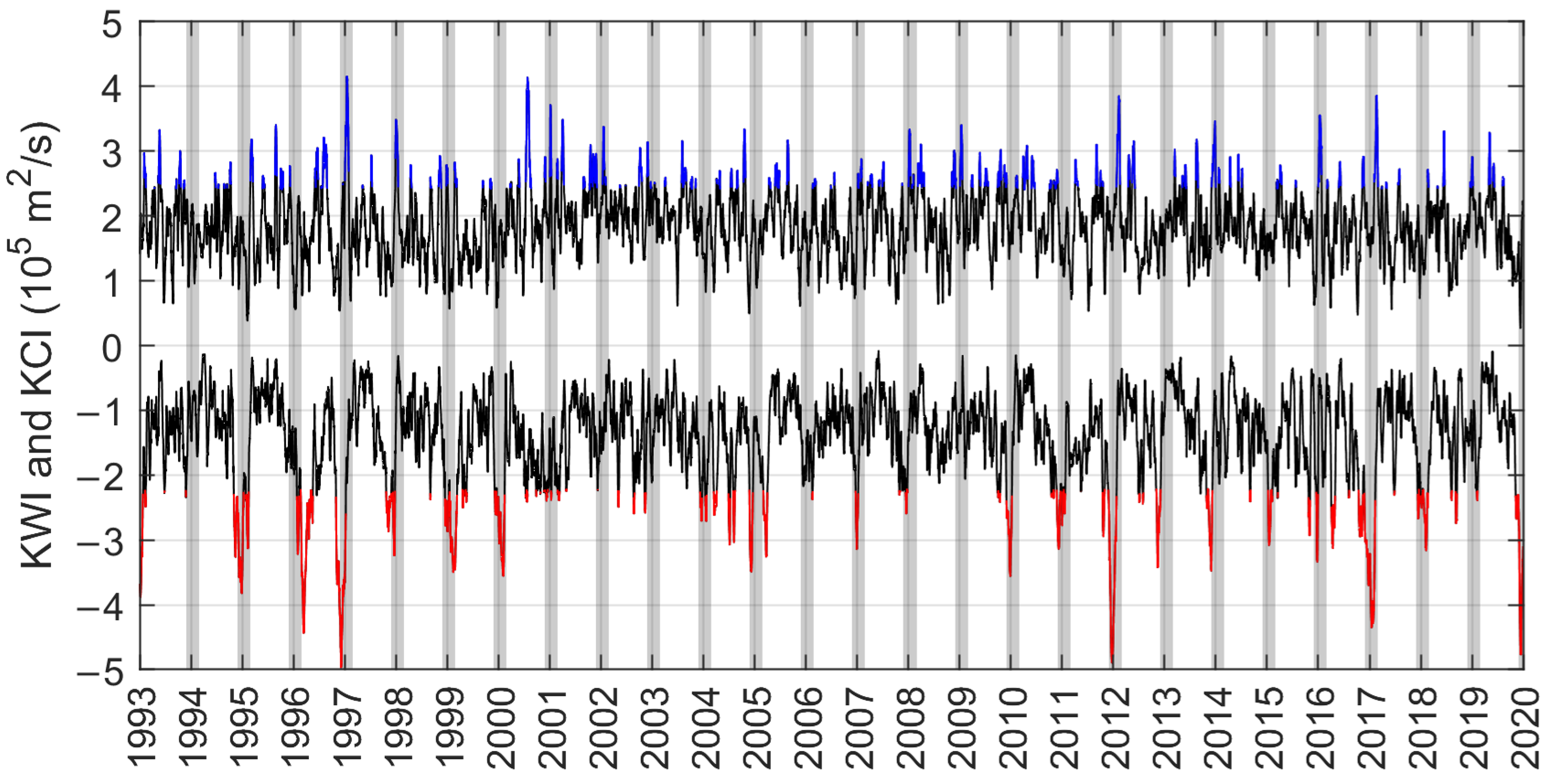
Values of information flow from KWI to AEKE in Box E10.0274−0.05650.02370.2069
Disclaimer/Publisher’s Note: The statements, opinions and data contained in all publications are solely those of the individual author(s) and contributor(s) and not of MDPI and/or the editor(s). MDPI and/or the editor(s) disclaim responsibility for any injury to people or property resulting from any ideas, methods, instructions or products referred to in the content.

