Article

Agricultural Land Cover Mapping through Two Deep Learning Models in the Framework of EU’s CAP Activities Using Sentinel-2 Multitemporal Imagery

by
Eleni Papadopoulou
1,
Giorgos Mallinis
2,*,
Sofia Siachalou
2,
Nikos Koutsias
3,
Athanasios C. Thanopoulos
4 and
Georgios Tsaklidis
1
1
Department of Mathematics, Aristotle University of Thessaloniki, 54124 Thessaloniki, Greece
2
School of Rural and Surveying Engineering, Aristotle University of Thessaloniki, 54124 Thessaloniki, Greece
3
Department of Sustainable Agriculture, University of Patras, 30100 Agrinio, Greece
4
Hellenic Statistical Authority (ELSTAT), 18510 Piraeus, Greece
*
Author to whom correspondence should be addressed.
Remote Sens. 2023, 15(19), 4657; https://doi.org/10.3390/rs15194657
Submission received: 23 August 2023 / Revised: 11 September 2023 / Accepted: 18 September 2023 / Published: 22 September 2023
(This article belongs to the Special Issue Explainable Artificial Intelligence (XAI) in Remote Sensing Big Data)

Abstract

:
The images of the Sentinel-2 constellation can help the verification process of farmers’ declarations, providing, among other things, accurate spatial explicit maps of the agricultural land cover. The aim of the study is to design, develop, and evaluate two deep learning (DL) architectures tailored for agricultural land cover and crop type mapping. The focus is on a detailed class scheme encompassing fifteen distinct classes, utilizing Sentinel-2 imagery acquired on a monthly basis throughout the year. The study’s geographical scope covers a diverse rural area in North Greece, situated within southeast Europe. These architectures are a Temporal Convolutional Neural Network (CNN) and a combination of a Recurrent and a 2D Convolutional Neural Network (R-CNN), and their accuracy is compared to the well-established Random Forest (RF) machine learning algorithm. The comparative approach is not restricted to simply presenting the results given by classification metrics, but it also assesses the uncertainty of the classification results using an entropy measure and the spatial distribution of the classification errors. Furthermore, the issue of sampling strategy for the extraction of the training set is highlighted, targeting the efficient handling of both the imbalance of the dataset and the spectral variability of instances among classes. The two developed deep learning architectures performed equally well, presenting an overall accuracy of 90.13% (Temporal CNN) and 90.18% (R-CNN), higher than the 86.31% overall accuracy of the RF approach. Finally, the Temporal CNN method presented a lower entropy value (6.63%), compared both to R-CNN (7.76%) and RF (28.94%) methods, indicating that both DL approaches should be considered for developing operational EO processing workflows.

Graphical Abstract

1. Introduction

Common Agricultural Policy (CAP), introduced as early as 1957 under the Treaty on the Functioning of the European Union, is one of the most important EU strategies, not only for receiving more than one-third of the EU’s budget, but also for supporting a range of socioeconomic, environmental, and political issues at an EU level and on a national scale. CAP serves as an instrument for improving agricultural productivity, meeting the expected demand for affordable, high-quality food provision [1] while preserving the natural environment [2].
In Europe, implementation of the CAP at national level is facilitated through the Land Parcel Identification System (LPIS), covering each Member State (MS) terrestrial territory [2]. LPIS is an information system that gathers information relevant to cropland at the parcel level [3]. It is regularly used for verifying applications and claims of the farmers through administrative and on-the-spot checks by responsible authorities, verifying eligibility criteria, and testing compliance with commitments and mandatory requirements [4]. The new regulation (Regulation (EU) 2018/746) adopted in 2018 for the CAP 2013–2020 transforms the verification process from the sample-based approach to an all-inclusive monitoring approach to the declarations.
Earth Observation is not relevant only to the verification of regulatory compliance, but it is also crucial for providing explicit spatial information essential for rural land management, food security [5], market trend forecasting, and analysis. The impact of changes in land use and consequently in land cover over time receives increasing attention since it concerns climate change, decline of biodiversity, degradation of water resources and soil, and outbreaks of infectious disease [6]. Not surprisingly, cropland and landcover mapping, based on EO data over rural areas, has been an active field of research over the past five decades. Cropland occupies a significant area in most European countries, and its utilization reflects the evolution towards the sustainable development and management of environmental resources [7,8]. That is why it is usually chosen to be examined in the framework of its spatial pattern. Throughout the years, an increasing number of studies have developed and evaluated diverse methodological approaches aiming to provide reliable, high accurate agricultural use and land cover information.
The temporal and spatial information of crop distribution is essential [9,10] in order to face several global challenges, such as climate change and increased food demand [11]. Satellite imagery provides data that allow near-real-time monitoring, serving the early detection of changes in land [12] and more effective terrain management. Contrary to manual labor, which demands effort and time and varies depending on the geographical region, remote sensing allows the creation of more accurate crop maps [9], which gather all necessary details for the amount and the type of agricultural fields. Spatial and temporal differences observed in crop growth, health, and yield are easily identified thanks to the evolvement of technology and the emergence of remote sensing data. Objectivity, timeliness, and accessibility in less accessible fields are some of the new potential [13] through aerial imagery. The analysis of these imagery is certainly faster and at a lower cost than the traditional methods of cropland mapping [14]. The issue of low resolution of the agricultural data collected by ground surveys is solved by the development and disposal of satellite observations in medium and high spatial resolution, which can cover broad areas of land across space and time [10]. Even if the resolution is not sufficient, it is possible to fuse images in order to augment it and identify ground objects at finer scales [15]. In most cases, the task of cropland mapping does not extend at a global scale since the classification algorithms cannot map all the existing types of crops as distinct classes [16].
The earlier paradigm of this domain relied on the use of the spectral information derived from single-date imagery on critical growth stages and the assumption that land cover and cropland types have distinct spectral signatures [17]. However, the spectral behavior of many crops is similar during the peak growing season period, and identifying the “optimal” sensing time is also challenging due to the crop development dynamics and the associated spectral changes within short time intervals [18]. To overcome misclassifications arising from the use of single-date imagery, classification approaches exploiting both the spectral and temporal information found in multitemporal remote sensing data have been proposed [17]. Multitemporal image acquisitions can be used to monitor and record spectral changes along the year, extracting information on the seasonality of vegetation, growth dynamics, and conditions [19]. Until the launch of the Sentinel-2A and Sentinel-2B data satellites in 2015 and 2017, respectively, multitemporal time series analysis was used on crop classification and rural mapping over large areas, mainly relying on the use of high temporal but low spatial resolution MODIS and medium temporal/spatial resolution Landsat data [20]. Crop and rural mapping becomes especially challenging with such data in heterogenous areas, as the Mediterranean rural landscapes are characterized by high fragmentation, small agricultural holdings, crop diversity, and within-crop spectral variability due to local weather conditions and topography [18]. On the other hand, the Sentinel-2 constellation, acquiring images with 10 m spatial resolution every 5–6 days around the globe, has the potential to provide detailed maps of agricultural land cover and is defined as the basic source of EO information in the case of 2020+ Common Agricultural Policy [20,21].
The improved characteristics of the new satellite systems also necessitate the development of new processing workflows that can support analysis of the spectral time series and streamline information extraction. Machine learning approaches such as the Random Forest (RF) algorithm have been employed successfully to exploit image time series in agricultural land cover studies [22,23]. In recent years, deep learning (DL) networks have been increasingly used by the EO community, increasing automation to multi-level feature representation and extraction as well as to end-to-end learning and information extraction without any need from the analyst to know the statistical distribution of the input data [24] and introduce features or rules manually [25]. It is common to be chosen as the preferred computing paradigm for several tasks since, in most cases, they can beat human labor in terms of effectiveness and time [26]. Among the several different DL architectures, such as deep belief networks [27,28], generative adversarial networks [29], transformers [30] and autoencoders [31,32], convolutional neural networks (CNNs) and recurrent neural networks (RNNs) are the most extensively used models for complex remote sensing applications [33,34]. Prominent examples are satellite image fusion for improved land use/land cover classification [35], object detection [36,37], and change detection [38,39] in remote sensing images, as well as the delineation of agricultural fields from satellite images [40]. CNNs are appealing to the remote sensing community due to their inherent nature to exploit the two-dimensional structure of images, efficiently extracting spectral and spatial features, while RNNs can handle sequential input in continuous dimensions with sequential long-range dependency, thus making them appropriate for the analysis of the spectral–temporal information in time series stacks [19,34,41,42,43,44].
In line with this evolvement and since the data and the algorithm design are two of the most significant factors for the success of the classification [
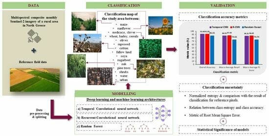
45], this paper describes the development of two different DL models for agricultural land cover and crop type mapping through a detailed fifteen class scheme in a heterogeneous area in Northern Greece, using a time series of Sentinel-2 images acquired in 2020. The two DL models, namely a Temporal CNN and an R-CNN are compared against an RF classifier, a robust machine learning algorithm used extensively in remote sensing studies. Given the high dependence of the success of these models on the data representation, a different, not so-common, type of standardization was tested and finally implemented on the reference instances. The modeling and predicting in the study area were limited to the spectral bands’ measurements of the raw data without integrating information from spectral indices derived from combinations of the existing bands. Overall, this study underlines the whole process of feature extraction, construction, and reforming using the smallest possible amount of satellite knowledge. Our study advances the field of remote sensing data mapping by employing an extended classification scheme in a complex, heterogeneous area, focusing on multiple crop types. To address known accuracy and reliability errors in reference data coming from farmers’ declarations [22,46,47,48] in our study, we relied only on recently verified ground reference data from the state agency managing such databases. The reference samples were used with optimized deep learning models to generate reliable and concrete findings. Finally, the novelty of our work is further reflected in our unique approach to assessing the results. Instead of relying solely on traditional measures of classification accuracy, we also calculate the Shannon entropy of class probability estimates. This approach defines accuracy not merely in conventional terms but also considers the entropy of all potential probabilities or votes toward different class labels for a pixel, serving as an innovative uncertainty measure. This dual analysis not only provides a comprehensive view of the classification but introduces a novel method of interpreting accuracy within the field.
The paper is organized as follows: Section 2 presents a brief introduction to the CNN and RNN architectures. Then, Section 3 presents the region of research, the reference data, the pre-processing, and the validation approach for the developed DL architectures. Section 4 reports the performance of the predictive models through certain evaluation metrics and visual representation of classification, as well as in terms of classification uncertainty. Section 5 discusses the results of this study in relation to earlier works, and finally, Section 6 summarizes the main findings and the conclusions of the whole work.
All the classification models were designed, trained, and evaluated efficiently on the CPU, while the writing and the execution of python code (version 3.8.8) were performed on Jupyter Notebook.

2. Feedforward and Recurrent Neural Networks

Depending on the flow of signals, NNs are divided into two types of topologies: the feedforward and the recurrent NNs (Figure 1). In this study, both topologies of neural networks are examined, with their proposed analytical architectures being presented in Section 3.

2.1. Feedforward Neural Networks and Temporal Convolutions

Feedforward neural networks are formed by various layers, known as dense or fully-connected layers, each of which includes a certain number of units-neurons. Each one of them is connected with all the units in the following layer, and any such connection is characterized by a weight.
The output of most of the layers, depending on their type, is produced after applying a function called the activation function. Non-linear or piecewise linear activation functions are the most preferred so that the NN is able to learn non-linear and complex mappings between its inputs and outputs [49].
If we suppose that there are N training instances, then the training set includes all the pairs of the form x ( k ) , d ( k ) R T * L x R C l . Thus, we have that X t r a i n = x ( 1 ) , d ( 1 ) , x ( 2 ) , d ( 2 ) , , x ( N ) , d ( N ) , where T is the length of each L -variate input time series x ( k ) , k = 1 , 2 , , N and C l is the number of classes. On the contrary, each vector d ( k ) , whose components are all zero except one component that equals 1, represents the output of a neural network. The unique value of 1 is placed in this index, which is equal to the class label of the training instance.
The aim of training an NN is the estimation of output vectors y ( k ) , k = 1 , 2 , , N to approximate, in the best way possible, the corresponding target vectors d ( k ) . That is why the criterion used to evaluate the model fitting to training data is the minimization of an error function, known as Cross-Entropy:
= 1 N × k = 1 N i = 1 C l d i k × l n y i k .
For this purpose, the network parameters, i.e., weights and biases of all layers, are updated after each training step according to an optimization algorithm using a subset of training data.
In a temporal convolutional layer, a series of filters known as convolutional kernels are applied to the two-dimensional output of the previous layer. Each filter is a matrix of weights that slides only across the height of the input of the current layer, being element-wise multiplied with a patch of a given size. Then, the individual products are summed together to produce a single number. The output of each filter is a one-dimensional feature map, whose size is given by
n H l = n H ( l 1 ) + 2 × p l f H ( l ) s ( l ) + 1 .  
The variable n H ( l ) represents the height of the representation of l th layer, whereas f H ( l ) corresponds to the height of each filter. The width of each convolutional kernel coincides with that of the layer’s input, which is why there is no reference to it. Furthermore, padding p l and stride s l are two additional hyper-parameters for l th layer, from which the first one is the number of zeros added at the edges of the layer’s input, and the second one is the step of the filter’s movement across one direction. In the end, the symbol . denotes the floor of the number inside it, i.e., the largest integer that is less than or equal to the inside value.
Figure 2 depicts the application of three convolutional kernels into a multivariate time series. The output representation consists of three stacked one-dimensional feature maps.

2.2. Recurrent Layers and 2D Convolutions

Long Short-Term Memory NN (LSTM), a particular class of RNNs, is a type of network of memory blocks that overcomes the limitation of exclusive learning of the short-term dependencies. At any given point in time, the LSTM unit consists of a memory cell and three gates: forget, input, and output. A forget gate establishes how much information derived from the previous time steps is significant, and an input gate controls the amount of the total imported input in the LSTM unit, which should pass into the memory cell and consequently should be memorized and used. On the contrary, an output gate assesses the content of memory, which will be exposed at the outside of the corresponding LSTM unit.
In recent years, research has begun into the efficiency of those NNs that combine the forward-backward nature of LSTM NNs and the spatial convolution of 2D Neural Networks. They have been designed and tested in several remote sensing applications, from the classification of satellite images [50,51] to change detection in land cover [52].
A filter used in a 2D convolutional layer is a 3D matrix (height width depth) and is element-wise multiplied by the same-sized patches of the layer’s input [53]. Its spatial dimensions are smaller than the corresponding dimensions of the input of this specific layer, leading to sliding over both the width and the height of the input volume. The weights are shared across all convolutions which use the same filter, resulting in a reduction of parameters compared to the use of a fully-connected layer.

3. Data and Methods

3.1. Study Area

The study area is located in the Prefecture of Serres in the northeastern part of Greece and covers diverse ecosystems of about 2341 km2. The landscape is mainly characterized by a flat agricultural area with various crop types (Table 1) and a hilly part captured by forests (principally oak and pine trees) and shrubland (Figure 3). Except for agricultural fields, several urban sub-regions are spread across the study area, while the Strymonas River flows into the Aegean Sea [54], affecting and contributing significantly to the economic growth of agriculture and livestock farming [55]. The climate of this region is continental [56], with dry and hot summers and wet and cold winters [57].
For 2019, according to the data of the Hellenic Statistical Authority in Greece, a total area of 32,165 km2 is covered by cultivated agricultural land. This total area consists of four main groups of crops, distributed as follows: 52.80% of the cultivated area was used for arable crops, 1.90% for horticultural cultivations, 33.80% for permanent crops, and 11.50% were fallow lands [58].
Table 1. Crop frequency (% of parcels) within the Prefecture of Serres [59].
Class Name Percent of Pixels
wheat, barley, cereals28.68%
fallow land 10.84%
cotton9.15%
olives8.76%
maize8.73%
sunflower/rapeseed/soya6.86%
nuts3.23%
horticultural 2.62%
rice1.02%
vineyards1.02%
The phenology of the crops in the investigated area is illustrated in Figure 4. Maize, sunflower, soya, sugarbeet, cotton, and soya are considered annual crops, and those fields are covered by dense vegetation during the summer months. On the other hand, class ‘wheat, barley, cereals’ is a spring crop, harvested before June while rapeseed later in July. Class ‘medicaco, clover’ may have 3–4 cuttings and flowerings per year, usually between May and September. The cropping pattern of the study area is considered heterogeneous regarding the agronomic practices and, specifically, the dates of planting, emergence, and harvesting. In the Table below, the most frequent classes of the Prefecture of Serres, as well as the percentage of the respective parcels, can be found.

3.2. Image Data

The image dataset consists of 12 Sentinel-2 (S2) monthly composite images generated through the Google Earth Engine (GEE) cloud platform [60,61]. The composites are formed upon individual Sentinel-2 level-2A scenes, which are available in Analysis Ready Data (ARD) format through GEE. The level-2A product provides Bottom Of Atmosphere (BOA) reflectance images, corrected for atmospheric influences. For each Sentinel-2 image, ten bands, resampled at 10 m spatial resolution, were used: Blue, Green, Red, Vegetation Red Edge 1, Vegetation Red Edge 2, Vegetation Red Edge 3, NIR-1, NIR-2, SWIR 1 and SWIR 2 (Table 2) [62].
The original spatial resolution of these bands varies from 10 to 20 m. In detail, four of these bands-three in the visible (Blue, Green, Red) and one in the near-infrared (NIR-1)-had spatial resolution of 10 m and six bands-three in the red-edge (Vegetation Red Edge 1, 2 and 3), one in the near-infrared (NIR-2) and two in the short-wave infrared (SWIR 1 and 2)-had spatial resolution of 20 m [63,64]. The presence and availability of three bands in the red-edge region part of the electromagnetic spectrum are particularly important since they can capture crop type differences and vegetation status [65,66]. This is another reason why a Sentinel-2 image time series was selected instead of other free satellite imagery, such as those provided by Landsat-8 and SPOT-4. Furthermore, 10 m Sentinel-2 data have the apparent benefit of offering more detailed information in comparison with 30 m or 20 m multispectral imagery supplied by Landsat-8 [67] and SPOT-4 [68], respectively.
Originally, the bitmask Quality Assessment (QA60) band was used in order to mask areas covered by clouds. Subsequently, the cloud-free images of 2020 were used to produce median monthly composites to capture vegetation dynamics required for agricultural land cover discrimination.

3.3. Reference Instances

Reference samples regarding crop types were extracted from parcels of the Greek LPIS of 2020 provided by OPEKEPE, the Greek Payment Authority of Common Agricultural Policy (C.A.P.) Aid Schemes. All the EU Member States are obliged to have a Land Parcel Identification System (LPIS), which works as a geospatial database of the agricultural parcels for which subsidies are requested. In Greece, OPEKEPE is responsible for the management of LPIS, gathering information related to the crop species, the area of the agricultural parcels, and the identity of the producer. Furthermore, it holds a vector file within the field boundaries of the declared parcels included [69].
Regarding the study area, the following 15 classes were included in this study: (1) maize, (2) sunflower, (3) medicaco, clover, (4) wheat, barley, cereals, (5) olives, (6) rapeseed, (7) cotton, (8) fallow land, (9) soya, (10) sugarbeet, (11) oak, (12) pine trees, (13) shrubs, (14) water, and (15) urban. The distribution of parcels and pixels in 15 classes is included in Table 3, proving that there is an imbalance among the number of instances per class, not only at the parcel level but also at the pixel level, both at training and test sets.
According to the splitting method, pixels included in 15% of the 1394 reference parcels are used for testing the models (Table 3). These parcels were selected after a stratified random sampling considering parcel distribution across classes. The remaining parcels were used for the training and validation of the classification models. Their architectures have been previously designated and evaluated by using a repeated (five times) stratified five-fold cross-validation, which aims to preserve diversity and avoid an unwanted loss of variance. This stratification is based again on the classes of the remaining parcels after the removal of testing parcels.

3.4. Data Pre-Processing

Each pixel instance, located in any x, y position in the satellite image series, is a vector composed of 120 components (12 Sentinel-2 images, each containing 10 bands). To be considered in the DL algorithms, each pixel is reformed into a 2D matrix with 12 × 10 dimensions (time band), highlighting its evolution over time.
As a second step, the values of 3D inputs of neural networks (number of instances number of time steps number of bands) are standardized according to a process that may be considered as a variant of the min–max normalization. As proposed by [70], the values of each band are subtracted by the 2nd percentile of all the values of the corresponding band belonging to training instances, and then the difference is divided by the range of the 98th percentile minus the 2nd percentile. The validation and test pixels are similarly modified, using the same values of percentiles. This type of standardization (as illustrated in Figure 5 for bands 4, 5, and 6) ensures that the temporal profile of spectral bands per class does not change. Merely, the order of magnitude changes, with most of the new values being within the range [−1, 1].

3.5. Temporal CNN Classification Model

The proposed Temporal CNN architecture has been optimized based on the 25 individual training and validation subsets [71]. Figure 6 shows the output dimensions of each layer of the Temporal-CNN. As presented below, the architecture is composed of three 1D convolutional layers with 128 filters of height equal to 3 each, a flattening layer, and two dense layers with 256 and 15 neurons, respectively. After each layer, except for the output layer, the technique of Batch Normalization is introduced, normalizing the activations [72], followed by the ReLU activation function, which is defined as R e L U x = max 0 , x . Among others, it has been proved that this function can achieve faster learning of a deep convolutional neural network than hyperbolic tangent [73]. After the application of the ReLU function, we integrate a dropout layer with a dropout rate of 0.5 [74]. In the output layer, the softmax activation function is applied because it has the advantage of converting the outputs into probabilities that sum to one. In particular, the output unit i for kth instance is given by the following formula:
y i ( k ) = s o f t m a x s i ( k ) = e x p s i ( k ) j = 1 C l e x p s j ( k ) , i = 1,2 , , C l , k = 1 , 2 , , N ,
where s i ( k ) is the ith component of the vector s ( k ) which contains the output values of the neural network’s previous layer for the kth instance.
We train this network using AMSGrad optimization [75] with hyper-parameter values: η = 10 4 ,   β 1 = 0.9 ,   β 2 = 0.999 , ϵ = 10 7 and a batch size of 32. An early stopping training mechanism is adopted, building on the minimization of loss function for validation instances and setting the maximum number of training epochs to 20.

3.6. R-CNN Classification Model

The proposed Recurrent-Convolutional Neural Network (Figure 7) is originally composed of a layer with LSTM memory blocks with peephole connections, each giving; as a result, an output of 32 units. This kind of peephole connection enables the memory cell at every time step to be linked to the gates [76]. A dropout layer with a dropout rate of 0.2 follows, and then, a time-distributed dense layer of 12 units is applied, maintaining the multidimensionality of the representations. This type of layer executes the function of a dense layer, differentiating it on the basis of application to every output of the previous layer throughout time. The output is reshaped in order to increase the dimension of the previous output from 2 to 3 and have the potential of extracting volumes through 2D convolutional layers. The first 2D convolutional layer applies 16 filters of size 5 × 5, producing an output volume that is fed in a Batch Normalization layer. The feature map passes through a dropout layer with the above-mentioned dropout rate, having already been changed due to the ReLU activation function. Subsequently, we repeat the same type of convolution in the produced output, using 32 kernels of 8 × 8. The padding is characterized, at both convolutional layers, as valid, meaning that no artificially generated zeros are added. In the last stage, we remove the unnecessary dimensions by flattening the feature tensor, and the result is mapped to 15 probabilities by means of a dense output layer of 15 units and a softmax activation function. In both NNs’ architectures, the same optimization algorithm (AMSGrad) is applied, setting the same values in the appropriate hyper-parameters.

3.7. Random Forests Benchmark Classification

Several remote sensing studies have reported that RF algorithms can handle high data dimensionality and provide improved classification results, in particular when working with multitemporal data [77]. RF is a nonparametric supervised learning method and consists of an ensemble of individual decision trees. At each tree, a bootstrap dataset is constructed with random sampling with replacement, evenly sized with the training dataset [78]. In this way, some instances are repeated in each decision tree. With the use of the selected training instances of each bootstrap dataset, the corresponding tree is built, forming decision rules between the inputs and the classes of classification [79]. In addition, each internal node further splits into child nodes based on the values of a particular feature, which is selected from a random feature subset of a predetermined size. The splitting criterion (e.g., the minimization of the Gini index) is defined by the user in view to quantify the quality of each split. This splitting procedure is repeated many times until each classification tree is fully constructed, ending at its leaves.
In the present study, the original dataset is separated appropriately on the basis of the reference parcels’ distribution among classes. After several trials, which are differentiated according to the number of trees, number of features, and maximum depth of each classification tree, we suggest that the RF should establish the outcome of classification using 400 trees and a maximum depth of 8 splits. This selection was directly related to the prevention of overfitting maintaining, at the same time, the validation accuracy as high as possible. Also, each randomly selected subset included 11 candidate splitting features, a number that is almost equal to the preferred, from theory, square root of the total number of features. The best splitting feature for each internal node is chosen under the minimization of Gini impurity, which is given using, for example, feature A, as follows:
G i n i s p l i t A = t = 1 k n ( t ) n × G i n i ( t ) ,
where k is the number of child nodes arising after the splitting and G i n i ( t ) represents the Gini index for node t , calculated by
G i n i t = 1 i = 1 C l p i t 2 .
We suppose that the set of classes is F = 1,2 , , C l and p i t is the fraction of the total number of instances of node t belonging to class i . Moreover, during the building of each tree, every internal node was split, demanding, at a minimum, two instances. The proposed architecture of RF was complemented by the introduction of a nonzero complexity parameter ccp_alpha, which was set to be equal to 10 3 .

3.8. Validation of the Results

3.8.1. Classification Accuracy Metrics

Accuracy assessment of any classification task of C l classes is commonly based on the formulation of the confusion matrix–i.e., a square matrix C of dimension C l C l . An element, C i , j ( i , j F = 1,2 , , C l ) , represents the number of instances of the given set which truly belong to class i and are predicted to belong to class j . The metric of overall accuracy (OA) is defined as
o v e r a l l   a c c u r a c y = i F C i , i i F j F C i , j .
An additional fundamental evaluation metric is the precision (or user’s accuracy) for a given class. It is calculated by dividing the number of correctly classified instances into this class by the number of instances predicted to belong to this class. Thus, the mathematical formula of its definition for a class k is
p r e c i s i o n k = C k , k i F C i , k .
Furthermore, another important metric is the so-called recall (or alternatively the producer’s accuracy). This is defined as the ratio between the number of correctly classified instances into a given class and the number of instances whose true class is this class. The metric of recall for the class k is given as
r e c a l l k = C k , k j F C k , j .
By means of recall values for all available classes, we computed macro average recall as their arithmetic mean:
m a c r o   a v e r a g e   r e c a l l = k F r e c a l l k C l .
The metric of macro F1 Score, described as the average of F1 Scores produced for each class, was also used in order to combine the information from precision and recall. The range of values for all metrics is the closed interval [0, 1], achieving a perfect classification of the instances when they approach 1.

3.8.2. Classification Uncertainty Evaluation

For the evaluation of the DL architectures, we accounted for the spatial distribution of the classification errors [80]. First, we compute the Shannon entropy of the discrete random variable D ( k ) , with k representing each pixel whose class of classification is known. The possible values of D ( k ) for each k are numbered in 15 and have a probability of class membership:
P D k = i x k = y i ( k ) ,
where the variable k belongs to the finite set 1 ,   2 ,   ,   172,744 and the variable i reflects the class of classification. In DL models, the values y i ( k ) are computed using a normalized exponential function named softmax, while in RF, they are calculated as the percentage of tree votes towards each class label.
The normalized Shannon entropy for an instance k is quantified by
n o r m a l i z e d   e n t r o p y D k = i = 0 14 y i k × l o g 2 y i k l o g 2 15 .
This value, for each instance, brings together all the appropriate information on membership values in all classes and demonstrates the uncertainty of its final class prediction. It varies from 0 to 1, with the ideal scenario occurring when the highest probability is assigned to the real class.
Finally, the correlation between values of normalized entropy and correct/incorrect classified classification of the reference pixels was assessed though the calculation of a variant of the metric RMSE [80]. A new variable r ( k ) for the representation of the classification result of instance k was developed, having two possible values: 0 for correct classification and 1 for incorrect classification.
The degree of deviation of the classes’ predictions of test pixels from the optimal behavior was defined as
R M S E = k = 1 n n o r m a l i z e d   e n t r o p y ( D k ) r ( k ) 2 n ,
where n is the number of test pixels, thus, from the point of uncertainty, the perfect state of an input is its correct classification with the lowest normalized entropy or its erroneous classification in parallel with the highest possible normalized entropy value.

4. Results

4.1. Classification Accuracy

Several trials of neural networks’ architectures have been carried out, altering the batch size, the complexity (associated with the number of layers and the number of the units in each layer), the filters’ size, the sequence of the above types of layers, the factor of kernel regularization, the optimization training algorithm’s hyper-parameters and the introduction or not of intermediate pooling layers of different types (1D average pooling, 1D max pooling, 1D global average pooling, 1D global max pooling). Furthermore, in the case of the RF, different numbers of trees, splitting features, maximum depth of each classification tree, weight of classes, and value of the complexity parameter were examined. The final architecture of each classification algorithm was chosen, taking into account as the main criterion the maximization of the validation accuracy (Figure 8), the minimization of the training time, and the trainable parameters (weights and biases) in the case of neural networks.
Ιt can be noticed that Temporal CNN and R-CNN have very close values of mean validation accuracy (Figure 8), with the 25 values being approximately equivalently varied around their average. More precisely, the Temporal CNN and R-CNN present the best performance (OA = 90.13% and OA = 90.18%, respectively), while the RF has a statistically significant difference in mean validation accuracy (Figure 8) in comparison with the remaining models (i.e., no overlapping of the corresponding standard deviation bars).
The metrics of overall accuracy, macro average recall, and macro average F1 Score [81] in the test set (Figure 9) also indicate the superiority of the two DL architectures when considering the test set. The overall accuracy is almost equal (~91.60%), while the R-CNN approach slightly outweighs in terms of macro average recall (87.44%) and macro average F1 Score (86.03%) the Temporal CNN approach (86.53% and 85.31% respectively). The relative change of the F1 score for the test set equals +0.84% between the two aforementioned models, whereas this is at around +15.11% between R-CNN and RF, in favor of R-CNN. This classification metric has been proven to be more useful and effective than overall classification accuracy in cases of class imbalance.
The metric of the F1 Score (Table 4) values per class for classification of the validation set, averaged by 25 runs of each algorithm, also suggests that Temporal CNN and R-CNN are almost equivalent. It is important to note that the Temporal CNN has equally good performance for both classes of limited size (e.g., pine trees) and frequent classes (e.g., cotton). The RF does not manage to reach the average levels of efficiency of the other two architectures, having the worst results in classes fallow land and sugar beet.
The lowest F1 Score for both DL algorithms is noted in the case of fallow land (59.30%), while both Temporal CNN and R-CNN provide moderate accuracy in the case of olive parcels (79.73% and 76.86%, respectively), which is, nevertheless, much higher, compared to the accuracy attained from the RF model (55.68%). A possible reason for the misclassification of fallow land by all the models might be the difficulty of its definition as a distinctive class [82]. In any case, the RF model seems to perform adequately in the case of agricultural land cover types, presenting significant phenological (and accordingly spectral) variation across the year, but its discriminatory ability is much compared to the DL models when it comes to crop mapping.
With a view to further assessing the efficiency of the three approaches, the classification results were visually evaluated within three sub-regions of the study area (Figure 10). The variants of classification schemes generated differentiated land cover products, with large area deviations being especially observed in the case of RF. Overall, the spatial distribution of the classes within the maps developed by the two DL models seems very similar, confirming the accuracy metrics findings. The RF map indicates the limitation of the approach both in crop-covered areas as well as in the case of more generic land-cover classes. More specifically, the approach generates more noisy output, underestimating urban areas (sub-regions B and C) and erroneously identifying pine areas as shrublands (sub-region C). In addition, the RF approach results in the misclassification (omission) of fallow land pixels (sub-region B), not exploiting information from the temporal spectral pattern of the specific class. Instead, these fields are incorrectly classified as wheat, barley, and cereals. In the case of both DL models, shrubland areas are incorrectly classified as olive tree parcels, as can be noted in the agricultural natural area fridge in sub-region C. This confirms the relatively low (Table 4) F1 Score (i.e., 76–79%) achieved for this class.

4.2. Classification Uncertainty

In Figure 11, it is underlined that the erroneous predictions are concentrated within the areas of increased normalized entropy. Moreover, when the model is one of Temporal CNN and R-CNN, the entropy’s values are kept at low levels, which is why lighter colors dominate. Moreover, it seems that RF’s architecture fails to produce results of high confidence. A potential reason might be the absence of a loss function which, in deep neural networks’ algorithms, takes into account both the predicted and the real distribution of training data. In addition, the RF’s architecture is the only one among all the proposed architectures that does not consider the temporal dimension of instances. Table 5 concentrates the values of averaged normalized entropy and classification accuracy of test pixels per class and classification model and confirms the superiority of neural networks over RF.
Table 5 demonstrates a negative relation between class entropy and class accuracy. For instance, classes sugar beet, fallow land, and olives demonstrate, at the same time, the highest uncertainty of classification and the lowest classification accuracy. These are among the classes which contain the lowest number of instances. Classes pine trees and urban constitute an exception because, even though they incorporated the least number of training instances, they do not have high uncertainty of classification. Class fallow land presents high spectral variability because each parcel may be plowed in a different period and does not follow a specific temporal pattern of growth.
Average entropy values indicated the Temporal CNN model managed to present results with lower confidence (entropy = 6.63%) compared to the respective R-CNN model (entropy = 7.76%).

4.3. Statistical Assessment

McNemar’s test is a statistical test and is commonly used in order to compare two different classifiers concerning their performance and consistency. It is designed to examine whether the predictions produced by the models for a given test set are statistically different [83]. Hence, the null hypothesis of this test claims equal performance between the two classification algorithms. It is a form of Chi-square test [84] with one degree of freedom [85], and the test statistic in a continuity-corrected version is computed using the cells of a 2 × 2 contingency table as follows [86]:
X 2 = n i , j n j , i 1 2 n i , j + n j , i .
The variable n i , j represents the number of instances classified correctly by the classifier i but not by the classifier j, while the variable n j , i is the number of misclassified instances applying the classifier i but classified correctly by the classifier j.
Table 6 concentrates the estimated values of McNemar’s test applied in the output classification results for test instances by all the models. Given the selection of the significance level at a = 0.05, it is apparent that we cannot reject the null hypothesis in the case of Temporal CNN and R-CNN. In other words, the fact that the p-value exceeds the value of 0.05 asserts that the difference in the performance of these two models is statistically insignificant. On the other hand, we can easily report that the RF’s algorithm produces statistically different output in the task of classification from both the neural networks’ architectures (Temporal CNN and R-CNN) since, in these two cases, the p-value is much smaller than the predefined significance level.

5. Discussion

The post-2020 reform of the CAP is based on the use of Earth Observation (EO) data in the crop-monitoring and eligibility verification process [20]. The EU’s Copernicus programme, providing freely distributed data with increased revisit capacity, spatial and spectral resolution, and systematic and frequent global coverage, is the main source of information used to support the implementation of the new CAP. The focus of this study was the development of two supervised DL classification methods for agricultural land cover mapping and crop classification using a Sentinel-2 image temporal dataset. In addition, we compared the two structures based on neural networks with a well-established RF algorithm. This machine learning approach was selected because it has been shown from prior research to produce successful results [87,88]. Architecture development for the two DL models was not a trivial task since identifying the optimal type of layers and the proper network structure (i.e., hyperparameters) is a rather subjective procedure not following standard approaches [19]. After the determination of the parameters’ values by means of cross-validation, we trained all three classifiers in order to test, afterward, their performance on the remaining test pixels.
The complexity of agriculture from the perspective of remote sensing can justify the implementation of monthly data. Different crop types usually follow diverse phenological cycles, with the stages and periods of growth not coinciding with one another. Even land parcels of the same crop type may appear to have dissimilar temporal and spectral behavior [87]. The selection of specific dates or seasons for the acquisition of image data [89,90], either being relevant to the phenological stages of the crops or suggested by certain algorithms, is proposed by many remote sensing studies in order to carry out the multitemporal classification. However, this fact can prevent the transferability of methodology to another region because the satellite imagery products downloaded at the chosen dates may be problematic for the desired task (cloudy conditions, similar spectral signature of classes) [91]. Thus, in order to facilitate the discrimination of crop types and support an operational land cover classification, we extended the examined annual time span to a monthly basis.
The chosen types of neural networks were far from random. It has been proven that Temporal Convolutional Neural Networks can work well with sequential data, while 2D CNNs obtain this possibility in parallel with automatic feature extraction after a combination of their architecture with recurrent layers. In addition, LSTMs learn both short-term and long-term dependencies, being free of the phenomenon of vanishing gradients. Yet, the classification scheme adopted in our study is challenging since only 10 out of the 15 classes correspond to crops. In that case, errors might be induced by DL algorithms focusing only on temporal feature representation and neglecting the spatial patterns derived from the 10 m data over the complex Mediterranean rural landscape.
The results indicated that both models performed exceptionally well, with a slight superiority of the R-CNN’s architecture over Temporal CNN’s, while RF appears to be unable to reach their classification performance. The combination of LSTM units with peephole connections and 2D convolutions achieved the highest macro average F1 Score of 86.03% in the validation set compared to 85.31% applying the Temporal CNN’s architecture. In the study of Zhong et al. [19], for classifying a 13-class crop scheme using enhanced vegetation index image stacks, a Conv1D-based model achieved higher accuracy compared to the best accuracy achieved by a model based on LSTM layers, although both models shared the same settings of dropout and fully-connected layers. Also, in the same study, the accuracy of both Conv1D and combined LSTM-Conv2D models was superior to the non-deep learning architecture. Also, Zhao et al. [92], in a study in North China for the discrimination of six different crops and forested areas using dense Sentinel-2 time series data, identified that 1D CNN slightly outperformed the LSTM models.
While both models attained similar classification accuracies, the assessment of the classification uncertainty indicated that the Temporal CNN model managed to assign individual pixels to be classified with lower uncertainty compared to the R-CNN model. It should be noted, as earlier studies highlight, that the CNN model presents less computational and time costs compared to LSTMs [14].
In regard to input features used for the classification task in our study, both models were developed using only the original bands of the Sentinel-2 images. Since our study involved different algorithms optimization and comparison, we avoided computing and using spectral indices, relying on previous research findings that suggested that additional features increase the input dimension and consequently the computational cost without significant improvement in classification accuracy [91]. Also, Cai et al. [17] and Xin et al. [93] identified limited improvement in terms of classification accuracy when using spectral indices along with the original bands for crop mapping.
However, this might not always be the case, and a significant body of the literature has identified and underlined the merits of considering spectral indices in the classification process. Zhong et al. [19] have identified that the use of a single spectral index as input to Temporal CNN-based models outperformed the result obtained from the full-band models. Yao et al. [94], through a feature space analysis, identified that spectral information of original bands was not adequate to distinguish crops, while original and modified (considering red-edge bands) NDVI indices were important for increasing class separability. Also, in a European-wide crop-type mapping study, yearly indicators based on spectral indices were deemed necessary for securing satisfactory classification accuracy compared to the original bands [95]. The importance of spectral indices as features for crop type mapping has also been identified in a study involving lower spatial resolution (i.e., MODIS) time series data for crop classification in the USA [96]. Based on the above findings, in the future and in order to address this limitation of our study, we will extend our approach by exploring in detail the importance of the spectral indices as explanatory features for increasing the classification accuracy of the study.
Earlier studies have developed DL models based on time series stacks of the original satellite images after cloud filtering (individual image approach) [17,97]. In our study, in order to minimize the data volume of the medium-high spatial resolution Sentinel-2 images and the associated computational cost, we employed a monthly composite method, which, based on the classification accuracy metrics, performed similarly to the individual-image approach. In addition, such a temporal composite approach might include fewer uncertainties when compared to, for example, the use of gap-filling interpolation methods, which may introduce erroneous observations in the time series and affect the robustness of the results [17].
The two DL models evaluated are not based on expert-rules or shape-fitting functions in order to incorporate information on temporal growth dynamics in the classification process, providing, thus, a robust, end-to-end approach for agricultural cover mapping [19].

6. Conclusions

Despite the scarcity of training samples and the existing diversity of crops in the study region, a classification with relatively high values in accuracy was achieved. The performance of modern time series forecasting algorithms, such as a Temporal Convolutional Neural Network and a 2D Convolutional Neural Network consisting of a layer with LSTM units with peephole connections, was compared with that of one of the most commonly used machine learning algorithms in remote sensing community, Random Forest. For this purpose, a novel multilevel methodological approach was proposed for land cover and crop type classification, including all the steps, starting with downloading and transforming raw satellite imagery and ending with predicting and monitoring the spatial distribution of land cover classes in the whole study area.
The way of splitting the reference instances into training, validation, and test subsets is crucial for the efficiency of feature learning and land cover estimation. In general, it is more prudent to split the available data on the basis of parcels’ distribution in classes. The fact that each object consists of pixels of similar spectral signature is a primary reason. In other words, when the model is trained using a number of pixels inside an object, and then it attempts to predict the class of another pixel belonging to the same object, the within-class variability of the pixels’ features in the object is negligible enough to guarantee the independence between the training and test instances.
Our model, which consists of both recurrent and convolutional layers, outperforms both the neural network being composed of 1D convolutional layers and the constructed RF in every measure being explored, except for overall accuracy. The difference in overall accuracy between the first two models is negligible, while the percentage difference regarding the macro average recall and macro average F1 Score between the R-CNN and each one of the remaining models is certainly higher.
Through the defined models’ architectures, fine-grained land cover maps were generated, with each class label being assigned to every pixel of the study area’s image. Furthermore, the additional representation of the uncertainty’s measurements in maps, in which the ambiguously classified areas were denoted as red, helped not only to the visual identification of certain problematic parcels but also to the discrimination of crop types in the rest sub-regions. It is very significant that the land cover maps can be further extended and interpreted to a percentage distribution of the classes covering the area, thus offering an alternative way of qualitative and quantitative evaluation that can be easily generalized at a global scale. This fact plays a key role in crop mapping, decision-making, and policy design for sustainable terrain management.
It is worth noting, as mentioned above, that it was attempted to find and capture possible correlations between the classes’ size, the accuracy per class, and the normalized entropy per class, with satisfactory conclusions. In test instances, classes such as ‘water’, ‘oak’, and ‘shrubs’ yielded amongst the lowest normalized entropies in conjunction with the highest accuracies, allowing their easy segmentation between all the classes. In summary, the RF architecture offered more uncertain predictions at the pixel level compared to those of neural networks. It seems that the size of the classes itself did not affect the confidence of the results, but the combination of the type of a class with its size might matter. As a result, a class containing only a few pixels, with its objects varying at a substantial degree (because of different agronomic practices), is expected that it will have higher normalized entropy.
Overall, this work integrated multitemporal and multispectral Sentinel-2 images combined with data from OPEKEPE for the classification of land cover on a particular region in Greece among 15 classes, most of which concern crop types. This discrimination was far from negligible since the chosen number was not so large to pose problems of confusion between similar crop classes (because of close spectral signature) and simultaneously not so small to lose the desired representative performance of the actual land distribution. Mapping the current study area was a challenging task due to its unique soil biodiversity as part of Mediterranean landscaping, especially when the data were generated by medium-resolution satellites. This area was not wholly within the boundaries of a specific city or a regional unit; that’s why its land combined diverse agricultural and management practices. Moreover, this study described a framework for land cover classification and cropland mapping, offering, in the end, operational products, such as a classification map at the pixel level, which are innovative for Greece. Despite the relatively low amount of labeled reference information, which was opposed to the demand of the developed algorithms, the results proved that the land distribution was successfully captured. Future research should consider exploring the discriminatory power of spectral indices as additional features to the original image bands for increasing the classification accuracy of the DL algorithms.

Author Contributions

Conceptualization, G.T., G.M., S.S. and E.P.; methodology, E.P., G.T., S.S. and G.M.; software, E.P.; validation, G.M., E.P. and S.S.; writing—original draft preparation, E.P.; writing—review and editing, G.M., E.P., G.T., S.S., N.K. and A.C.T.; supervision, G.T. All authors have read and agreed to the published version of the manuscript.

Funding

This research received no external funding.

Data Availability Statement

Data available on request.

Acknowledgments

We would like to thank OPEKEPE, the Greek Payment Authority of Common Agricultural Policy, for providing reference ground truth data. Sentinel-2 MSI data used were available at no cost from ESA Sentinels Scientific Data Hub. Figure 3, Figure 10 and Figure 11 contain modified Copernicus Sentinel data (2020).

Conflicts of Interest

The authors declare no conflict of interest.

References

  1. European Commission. The Common Agricultural Policy at a Glance. Available online: https://agriculture.ec.europa.eu/common-agricultural-policy/cap-overview/cap-glance_en#cap2023-27 (accessed on 9 August 2023).
  2. Tóth, K.; Kučas, A. Spatial Information in European Agricultural Data Management. Requirements and Interoperability Supported by a Domain Model. Land Use Policy 2016, 57, 64–79. [Google Scholar] [CrossRef]
  3. Xia, J.; Yokoya, N.; Adriano, B.; Kanemoto, K. National High-Resolution Cropland Classification of Japan with Agricultural Census Information and Multi-Temporal Multi-Modality Datasets. Int. J. Appl. Earth Obs. Geoinf. 2023, 117, 103193. [Google Scholar] [CrossRef]
  4. Sarvia, F.; Xausa, E.; De Petris, S.; Cantamessa, G.; Borgogno-Mondino, E. A Possible Role of Copernicus Sentinel-2 Data to Support Common Agricultural Policy Controls in Agriculture. Agronomy 2021, 11, 110. [Google Scholar] [CrossRef]
  5. Abubakar, G.A.; Wang, K.; Shahtahamssebi, A.; Xue, X.; Belete, M.; Gudo, A.J.A.; Shuka, K.A.M.; Gan, M. Mapping Maize Fields by Using Multi-Temporal Sentinel-1A and Sentinel-2A Images in Makarfi, Northern Nigeria, Africa. Sustainability 2020, 12, 2539. [Google Scholar] [CrossRef]
  6. Foley, J.A.; Defries, R.S.; Asner, G.P.; Barford, C.C.; Bonan, G.; Carpenter, S.R.; Chapin, F.S.; Coe, M.T.; Daily, G.C.; Gibbs, H.K.; et al. Global Consequences of Land Use. Science 2005, 309, 570–574. [Google Scholar] [CrossRef]
  7. Xue, J.; Zhang, X.; Chen, S.; Hu, B.; Wang, N.; Shi, Z. Quantifying the Agreement and Accuracy Characteristics of Four Satellite-Based LULC Products for Cropland Classification in China. J. Integr. Agric. 2023, 1–23. [Google Scholar] [CrossRef]
  8. Cai, T.; Luo, X.; Fan, L.; Han, J.; Zhang, X. The Impact of Cropland Use Changes on Terrestrial Ecosystem Services Value in Newly Added Cropland Hotspots in China during 2000–2020. Land 2022, 11, 2294. [Google Scholar] [CrossRef]
  9. Faqe Ibrahim, G.R.; Rasul, A.; Abdullah, H. Improving Crop Classification Accuracy with Integrated Sentinel-1 and Sentinel-2 Data: A Case Study of Barley and Wheat. J. Geovisualization Spat. Anal. 2023, 7, 22. [Google Scholar] [CrossRef]
  10. Li, H.; Song, X.-P.; Hansen, M.C.; Becker-Reshef, I.; Adusei, B.; Pickering, J.; Wang, L.; Wang, L.; Lin, Z.; Zalles, V.; et al. Development of a 10-m Resolution Maize and Soybean Map over China: Matching Satellite-Based Crop Classification with Sample-Based Area Estimation. Remote Sens. Environ. 2023, 294, 113623. [Google Scholar] [CrossRef]
  11. Heupel, K.; Spengler, D.; Itzerott, S. A Progressive Crop-Type Classification Using Multitemporal Remote Sensing Data and Phenological Information. PFG-J. Photogramm. Remote Sens. Geoinf. Sci. 2018, 86, 53–69. [Google Scholar] [CrossRef]
  12. Wheeler, T.; Von Braun, J. Climate Change Impacts on Global Food Security. Science 2013, 341, 508–513. [Google Scholar] [CrossRef] [PubMed]
  13. Wu, S.; Cao, L.; Xu, D.; Zhao, C. Historical Eco-Environmental Quality Mapping in China with Multi-Source Data Fusion. Appl. Sci. 2023, 13, 8051. [Google Scholar] [CrossRef]
  14. Ghayour, L.; Neshat, A.; Paryani, S.; Shahabi, H.; Shirzadi, A.; Chen, W.; Al-Ansari, N.; Geertsema, M.; Pourmehdi Amiri, M.; Gholamnia, M.; et al. Performance Evaluation of Sentinel-2 and Landsat 8 OLI Data for Land Cover/Use Classification Using a Comparison between Machine Learning Algorithms. Remote Sens. 2021, 13, 1349. [Google Scholar] [CrossRef]
  15. Ma, Z.; Li, W.; Warner, T.A.; He, C.; Wang, X.; Zhang, Y.; Guo, C.; Cheng, T.; Zhu, Y.; Cao, W.; et al. A Framework Combined Stacking Ensemble Algorithm to Classify Crop in Complex Agricultural Landscape of High Altitude Regions with Gaofen-6 Imagery and Elevation Data. Int. J. Appl. Earth Obs. Geoinf. 2023, 122, 103386. [Google Scholar] [CrossRef]
  16. Weiss, M.; Jacob, F.; Duveiller, G. Remote Sensing for Agricultural Applications: A Meta-Review. Remote Sens. Environ. 2020, 236, 111402. [Google Scholar] [CrossRef]
  17. Cai, Y.; Guan, K.; Peng, J.; Wang, S.; Seifert, C.; Wardlow, B.; Li, Z. A High-Performance and in-Season Classification System of Field-Level Crop Types Using Time-Series Landsat Data and a Machine Learning Approach. Remote Sens. Environ. 2018, 210, 35–47. [Google Scholar] [CrossRef]
  18. Siachalou, S.; Mallinis, G.; Tsakiri-Strati, M. Analysis of Time-Series Spectral Index Data to Enhance Crop Identification Over a Mediterranean Rural Landscape. IEEE Geosci. Remote Sens. Lett. 2017, 14, 1508–1512. [Google Scholar] [CrossRef]
  19. Zhong, L.; Hu, L.; Zhou, H. Deep Learning Based Multi-Temporal Crop Classification. Remote Sens. Environ. 2019, 221, 430–443. [Google Scholar] [CrossRef]
  20. Campos-Taberner, M.; Garcia-Haro, F.J.; Martinez, B.; Sánchez-Ruíz, S.; Gilabert, M.A. A Copernicus Sentinel-1 and Sentinel-2 Classification Framework for the 2020+ European Common Agricultural Policy: A Case Study in València (Spain). Agronomy 2019, 9, 556. [Google Scholar] [CrossRef]
  21. López-Andreu, F.J.; Erena, M.; Dominguez-Gómez, J.A.; López-Morales, J.A. Sentinel-2 Images and Machine Learning as Tool for Monitoring of the Common Agricultural Policy: Calasparra Rice as a Case Study. Agronomy 2021, 11, 621. [Google Scholar] [CrossRef]
  22. Blickensdörfer, L.; Schwieder, M.; Pflugmacher, D.; Nendel, C.; Erasmi, S.; Hostert, P. Mapping of Crop Types and Crop Sequences with Combined Time Series of Sentinel-1, Sentinel-2 and Landsat 8 Data for Germany. Remote Sens. Environ. 2022, 269, 112831. [Google Scholar] [CrossRef]
  23. Phalke, A.R.; Özdoğan, M.; Thenkabail, P.S.; Erickson, T.; Gorelick, N.; Yadav, K.; Congalton, R.G. Mapping Croplands of Europe, Middle East, Russia, and Central Asia Using Landsat, Random Forest, and Google Earth Engine. ISPRS J. Photogramm. Remote Sens. 2020, 167, 104–122. [Google Scholar] [CrossRef]
  24. Ahmad, M.; Shabbir, S.; Roy, S.K.; Hong, D.; Wu, X.; Yao, J.; Khan, A.M.; Mazzara, M.; Distefano, S.; Chanussot, J. Hyperspectral Image Classification—Traditional to Deep Models: A Survey for Future Prospects. IEEE J. Sel. Top. Appl. Earth Obs. Remote Sens. 2022, 15, 968–999. [Google Scholar] [CrossRef]
  25. Zhu, X.X.; Tuia, D.; Mou, L.; Xia, G.-S.; Zhang, L.; Xu, F.; Fraundorfer, F. Deep Learning in Remote Sensing: A Comprehensive Review and List of Resources. IEEE Geosci. Remote Sens. Mag. 2017, 5, 8–36. [Google Scholar] [CrossRef]
  26. Guo, Y.; Yu, Q.; Gao, Y.; Liu, X.; Li, C. Max-Min Distance Embedding for Unsupervised Hyperspectral Image Classification in the Satellite Internet of Things System. Internet Things 2023, 22, 100775. [Google Scholar] [CrossRef]
  27. Cao, T. Effective Detection Algorithm of Electronic Information and Signal Processing Based on Multi-Sensor Data Fusion. Egypt. J. Remote Sens. Space Sci. 2023, 26, 519–526. [Google Scholar] [CrossRef]
  28. Xu, C.; Lin, M.; Fang, Q.; Chen, J.; Yue, Q.; Xia, J. Air Temperature Estimation over Winter Wheat Fields by Integrating Machine Learning and Remote Sensing Techniques. Int. J. Appl. Earth Obs. Geoinf. 2023, 122, 103416. [Google Scholar] [CrossRef]
  29. Xu, Y.; Luo, W.; Hu, A.; Xie, Z.; Xie, X.; Tao, L. TE-SAGAN: An Improved Generative Adversarial Network for Remote Sensing Super-Resolution Images. Remote Sens. 2022, 14, 2425. [Google Scholar] [CrossRef]
  30. Bazi, Y.; Bashmal, L.; Rahhal, M.M.A.; Dayil, R.A.; Ajlan, N.A. Vision Transformers for Remote Sensing Image Classification. Remote Sens. 2021, 13, 516. [Google Scholar] [CrossRef]
  31. Dabboor, M.; Atteia, G.; Meshoul, S.; Alayed, W. Deep Learning-Based Framework for Soil Moisture Content Retrieval of Bare Soil from Satellite Data. Remote Sens. 2023, 15, 1916. [Google Scholar] [CrossRef]
  32. Odebiri, O.; Mutanga, O.; Odindi, J.; Naicker, R. Mapping Soil Organic Carbon Distribution across South Africa’s Major Biomes Using Remote Sensing-Topo-Climatic Covariates and Concrete Autoencoder-Deep Neural Networks. Sci. Total Environ. 2023, 865, 161150. [Google Scholar] [CrossRef] [PubMed]
  33. Shakya, A.; Biswas, M.; Pal, M. Parametric Study of Convolutional Neural Network Based Remote Sensing Image Classification. Int. J. Remote Sens. 2021, 42, 2663–2685. [Google Scholar] [CrossRef]
  34. Ma, L.; Liu, Y.; Zhang, X.; Ye, Y.; Yin, G.; Johnson, B.A. Deep Learning in Remote Sensing Applications: A Meta-Analysis and Review. ISPRS J. Photogramm. Remote Sens. 2019, 152, 166–177. [Google Scholar] [CrossRef]
  35. Shakya, A.; Biswas, M.; Pal, M. Evaluating the Potential of Pyramid-Based Fusion Coupled with Convolutional Neural Network for Satellite Image Classification. Arab. J. Geosci. 2022, 15, 759. [Google Scholar] [CrossRef]
  36. Chen, Y.; Lin, M.; He, Z.; Polat, K.; Alhudhaif, A.; Alenezi, F. Consistency- and Dependence-Guided Knowledge Distillation for Object Detection in Remote Sensing Images. Expert Syst. Appl. 2023, 229, 120519. [Google Scholar] [CrossRef]
  37. Li, W.; Zhou, J.; Li, X.; Cao, Y.; Jin, G. Few-Shot Object Detection on Aerial Imagery via Deep Metric Learning and Knowledge Inheritance. Int. J. Appl. Earth Obs. Geoinf. 2023, 122, 103397. [Google Scholar] [CrossRef]
  38. Zhao, H.; Feng, K.; Wu, Y.; Gong, M. An Efficient Feature Extraction Network for Unsupervised Hyperspectral Change Detection. Remote Sens. 2022, 14, 4646. [Google Scholar] [CrossRef]
  39. Ding, J.; Li, X. A Spatial-Spectral-Temporal Attention Method for Hyperspectral Image Change Detection. In Proceedings of the IEEE International Geoscience and Remote Sensing Symposium (IGARSS), Kuala Lumpur, Malaysia, 17–22 July 2022; Institute of Electrical and Electronics Engineers (IEEE): Piscataway, NJ, USA, 2022; pp. 3704–3707. [Google Scholar]
  40. Tetteh, G.O.; Schwieder, M.; Erasmi, S.; Conrad, C.; Gocht, A. Comparison of an Optimised Multiresolution Segmentation Approach with Deep Neural Networks for Delineating Agricultural Fields from Sentinel-2 Images. PFG-J. Photogramm. Remote Sens. Geoinf. Sci. 2023, 91, 295–312. [Google Scholar] [CrossRef]
  41. LeCun, Y.; Bengio, Y.; Hinton, G. Deep Learning. Nature 2015, 521, 436–444. [Google Scholar] [CrossRef]
  42. Parajuli, J.; Fernandez-Beltran, R.; Kang, J.; Pla, F. Attentional Dense Convolutional Neural Network for Water Body Extraction From Sentinel-2 Images. IEEE J. Sel. Top. Appl. Earth Obs. Remote Sens. 2022, 15, 6804–6816. [Google Scholar] [CrossRef]
  43. Zhao, L.; Ji, S. CNN, RNN, or ViT? An Evaluation of Different Deep Learning Architectures for Spatio-Temporal Representation of Sentinel Time Series. IEEE J. Sel. Top. Appl. Earth Obs. Remote Sens. 2023, 16, 44–56. [Google Scholar] [CrossRef]
  44. Li, B.; Guo, Y.; Yang, J.; Wang, L.; Wang, Y.; An, W. Gated Recurrent Multiattention Network for VHR Remote Sensing Image Classification. IEEE Trans. Geosci. Remote Sens. 2022, 60, 5606113. [Google Scholar] [CrossRef]
  45. Sun, X.; Wang, B.; Wang, Z.; Li, H.; Li, H.; Fu, K. Research Progress on Few-Shot Learning for Remote Sensing Image Interpretation. IEEE J. Sel. Top. Appl. Earth Obs. Remote Sens. 2021, 14, 2387–2402. [Google Scholar] [CrossRef]
  46. Asam, S.; Gessner, U.; Almengor González, R.; Wenzl, M.; Kriese, J.; Kuenzer, C. Mapping Crop Types of Germany by Combining Temporal Statistical Metrics of Sentinel-1 and Sentinel-2 Time Series with LPIS Data. Remote Sens. 2022, 14, 2981. [Google Scholar] [CrossRef]
  47. Erdanaev, E.; Kappas, M.; Wyss, D. Irrigated Crop Types Mapping in Tashkent Province of Uzbekistan with Remote Sensing-Based Classification Methods. Sensors 2022, 22, 5683. [Google Scholar] [CrossRef]
  48. Gounari, O.; Karakizi, C.; Karantzalos, K. Filtering Lpis Data for Building Trustworthy Training Datasets for Crop Type Mapping: A Case Study in Greece. In Proceedings of the International Archives of the Photogrammetry, Remote Sensing and Spatial Information Sciences, Nice, France, 6–11 June 2022; Volume XLIII-B3-2022, pp. 871–877. [Google Scholar]
  49. Khan, S.; Rahmani, H.; Shah, S.A.A.; Bennamoun, M. A Guide to Convolutional Neural Networks for Computer Vision, 1st ed.; Synthesis Lectures on Computer Vision; Morgan & Claypool Publishers: Kentfield, CA, USA, 2018; Volume 8. [Google Scholar]
  50. Mazzia, V.; Khaliq, A.; Chiaberge, M. Improvement in Land Cover and Crop Classification Based on Temporal Features Learning from Sentinel-2 Data Using Recurrent-Convolutional Neural Network (R-CNN). Appl. Sci. 2020, 10, 238. [Google Scholar] [CrossRef]
  51. Rußwurm, M.; Körner, M. Convolutional LSTMs for Cloud-Robust Segmentation of Remote Sensing Imagery. arXiv 2018, arXiv:1811.02471. [Google Scholar] [CrossRef]
  52. Mou, L.; Bruzzone, L.; Zhu, X. Learning Spectral-Spatial-Temporal Features via a Recurrent Convolutional Neural Network for Change Detection in Multispectral Imagery. IEEE Trans. Geosci. Remote Sens. 2018, 57, 924–935. [Google Scholar] [CrossRef]
  53. CS231n Convolutional Neural Networks for Visual Recognition. Available online: https://cs231n.github.io/convolutional-networks/#conv (accessed on 9 August 2023).
  54. Capolongo, D.; Refice, A.; Bocchiola, D.; D’Addabbo, A.; Vouvalidis, K.; Soncini, A.; Zingaro, M.; Bovenga, F.; Stamatopoulos, L. Coupling Multitemporal Remote Sensing with Geomorphology and Hydrological Modeling for Post Flood Recovery in the Strymonas Dammed River Basin (Greece). Sci. Total Environ. 2019, 651, 1958–1968. [Google Scholar] [CrossRef] [PubMed]
  55. N.E.C.C.A. Management Unit of Protected Areas of Central Macedonia. Available online: https://necca.gov.gr/en/mdpp/management-unit-of-koroneia-volvi-kerkini-and-thermaikos-national-parks-and-protected-areas-of-central-macedonia/ (accessed on 9 August 2023).
  56. Struma/Strymon River Sub-Basin. Available online: http://www.inweb.gr/workshops2/sub_basins/11_Strymon.html (accessed on 9 August 2023).
  57. Weather Spark. Climate and Average Weather Year Round in Sérres. Available online: https://weatherspark.com/y/89459/Average-Weather-in-S%C3%A9rres-Greece-Year-Round (accessed on 9 August 2023).
  58. Hellenic Statistical Authority. Areas and Production/2019. Available online: https://www.statistics.gr/en/statistics/-/publication/SPG06/2019 (accessed on 2 September 2023).
  59. OPEKEPE. Συγκεντρωτικά Στοιχεία Ενιαίων Aιτήσεων Εκμετάλλευσης. Available online: http://aggregate.opekepe.gr/ (accessed on 2 September 2023).
  60. Google. Google Earth Engine. Available online: https://earthengine.google.com/ (accessed on 9 August 2023).
  61. Amani, M.; Ghorbanian, A.; Ahmadi, S.A.; Kakooei, M.; Moghimi, A.; Mirmazloumi, S.M.; Moghaddam, S.H.A.; Mahdavi, S.; Ghahremanloo, M.; Parsian, S.; et al. Google Earth Engine Cloud Computing Platform for Remote Sensing Big Data Applications: A Comprehensive Review. IEEE J. Sel. Top. Appl. Earth Obs. Remote Sens. 2020, 13, 5326–5350. [Google Scholar] [CrossRef]
  62. European Space Agency. Resolution and Swath. Available online: https://sentinels.copernicus.eu/web/sentinel/missions/sentinel-2/instrument-payload/resolution-and-swath (accessed on 9 August 2023).
  63. Zabalza, M.; Bernardini, A. Super-Resolution of Sentinel-2 Images Using a Spectral Attention Mechanism. Remote Sens. 2022, 14, 2890. [Google Scholar] [CrossRef]
  64. Mancino, G.; Falciano, A.; Console, R.; Trivigno, M.L. Comparison between Parametric and Non-Parametric Supervised Land Cover Classifications of Sentinel-2 MSI and Landsat-8 OLI Data. Geographies 2023, 3, 82–109. [Google Scholar] [CrossRef]
  65. Immitzer, M.; Vuolo, F.; Atzberger, C. First Experience with Sentinel-2 Data for Crop and Tree Species Classifications in Central Europe. Remote Sens. 2016, 8, 166. [Google Scholar] [CrossRef]
  66. Schuster, C.; Förster, M.; Kleinschmit, B. Testing the Red Edge Channel for Improving Land-Use Classifications Based on High-Resolution Multi-Spectral Satellite Data. Int. J. Remote Sens. 2012, 33, 5583–5599. [Google Scholar] [CrossRef]
  67. USGS. Landsat 8. Available online: https://www.usgs.gov/landsat-missions/landsat-8 (accessed on 9 August 2023).
  68. European Space Agency. SPOT 4. Available online: https://earth.esa.int/eogateway/missions/spot-4 (accessed on 9 August 2023).
  69. Siachalou, S. Time Series Processing and Analysis of Satellite Images for Land Use/Land Cover Classification and Change Detection. Ph.D. Thesis, Aristotle University of Thessaloniki, Thessaloniki, Greece, 2016. [Google Scholar]
  70. Pelletier, C.; Webb, G.I.; Petitjean, F. Temporal Convolutional Neural Network for the Classification of Satellite Image Time Series. Remote Sens. 2019, 11, 523. [Google Scholar] [CrossRef]
  71. Aghdam, H.H.; Heravi, E.J. Guide to Convolutional Neural Networks: A Practical Application to Traffic-Sign Detection and Classification, 1st ed.; Springer: Cham, Switzerland, 2017. [Google Scholar]
  72. Ioffe, S.; Szegedy, C. Batch Normalization: Accelerating Deep Network Training by Reducing Internal Covariate Shift. In Proceedings of the 32nd International Conference on Machine Learning, Lille, France, 6–11 July 2015; JMLR.org: Lille, France; Volume 37, pp. 448–456. [Google Scholar]
  73. Krizhevsky, A.; Sutskever, I.; Hinton, G.E. ImageΝet Classification with Deep Convolutional Neural Networks. In Proceedings of the 25th International Conference on Neural Information Processing Systems, Lake Tahoe, NV, USA, 3–6 December 2012; pp. 1097–1105. [Google Scholar]
  74. Srivastava, N.; Hinton, G.; Krizhevsky, A.; Sutskever, I.; Salakhutdinov, R. Dropout: A Simple Way to Prevent Neural Network Overfitting. J. Mach. Learn. Res. 2014, 15, 1929–1958. [Google Scholar]
  75. Reddi, S.J.; Kale, S.; Kumar, S. On the Convergence of Adam and Beyond. In Proceedings of the 6th International Conference on Learning Representations, Vancouver, BC, Canada, 30 April–3 May 2018; pp. 1–23. [Google Scholar]
  76. Gers, F.A.; Schraudolph, N.N.; Schmidhuber, J. Learning Precise Timing with LSTM Recurrent Networks. J. Mach. Learn. Res. 2003, 3, 115–143. [Google Scholar] [CrossRef]
  77. Pal, M. Random Forest Classifier for Remote Sensing Classification. Int. J. Remote Sens. 2005, 26, 217–222. [Google Scholar] [CrossRef]
  78. Duchscherer, S.E. Classifying Building Usages: A Machine Learning Approach on Building Extractions. Master’s Thesis, University of Tennessee, Knoxville, TN, USA, 2018. [Google Scholar]
  79. Safavian, S.R.; Landgrebe, D. A Survey of Decision Tree Classifier Methodology. IEEE Trans. Syst. Man Cybern. 1991, 21, 660–674. [Google Scholar] [CrossRef]
  80. Roodposhti, M.S.; Aryal, J.; Lucieer, A.; Bryan, B.A. Uncertainty Assessment of Hyperspectral Image Classification: Deep Learning vs. Random Forest. Entropy 2019, 21, 78. [Google Scholar] [CrossRef]
  81. Grandini, M.; Bagli, E.; Visani, G. Metrics for Multi-Class Classification: An Overview. arXiv 2020, arXiv:2008.05756. [Google Scholar] [CrossRef]
  82. Rußwurm, M.; Körner, M. Temporal Vegetation Modelling Using Long Short-Term Memory Networks for Crop Identification from Medium-Resolution Multi-Spectral Satellite Images. In Proceedings of the 2017 IEEE Conference on Computer Vision and Pattern Recognition Workshops (CVPRW), Honolulu, HI, USA, 21–26 July 2017; pp. 1496–1504. [Google Scholar]
  83. Özdemir, H.; Baduna Koçyiğit, M.; Akay, D. Flood Susceptibility Mapping with Ensemble Machine Learning: A Case of Eastern Mediterranean Basin, Türkiye. Stoch. Environ. Res. Risk Assess. 2023, 1–18. [Google Scholar] [CrossRef]
  84. Nakata, N.; Siina, T. Ensemble Learning of Multiple Models Using Deep Learning for Multiclass Classification of Ultrasound Images of Hepatic Masses. Bioengineering 2023, 10, 69. [Google Scholar] [CrossRef] [PubMed]
  85. Zablan, C.D.; Blanco, A.; Nadaoka, K.; Martinez, K. Assessment of Mangrove Extent Extraction Accuracy of Threshold Segmentation-Based Indices Using Sentinel Imagery. In Proceedings of the International Archives of the Photogrammetry, Remote Sensing and Spatial Information Sciences, Johor Bahru, Malaysia, 14–17 November 2022; International Society for Photogrammetry and Remote Sensing: Bethesda, MD, USA, 2022; Volume 48, pp. 391–401. [Google Scholar]
  86. Iban, M.C.; Sekertekin, A. Machine Learning Based Wildfire Susceptibility Mapping Using Remotely Sensed Fire Data and GIS: A Case Study of Adana and Mersin Provinces, Turkey. Ecol. Inform. 2022, 69, 101647. [Google Scholar] [CrossRef]
  87. Griffiths, P.; Nendel, C.; Hostert, P. Intra-Annual Reflectance Composites from Sentinel-2 and Landsat for National-Scale Crop and Land Cover Mapping. Remote Sens. Environ. 2019, 220, 135–151. [Google Scholar] [CrossRef]
  88. Xiong, J.; Thenkabail, P.S.; Tilton, J.C.; Gumma, M.K.; Teluguntla, P.; Oliphant, A.; Congalton, R.G.; Yadav, K.; Gorelick, N. Nominal 30-m Cropland Extent Map of Continental Africa by Integrating Pixel-Based and Object-Based Algorithms Using Sentinel-2 and Landsat-8 Data on Google Earth Engine. Remote Sens. 2017, 9, 1065. [Google Scholar] [CrossRef]
  89. Rodriguez-Galiano, V.F.; Ghimire, B.; Rogan, J.; Chica-Olmo, M.; Rigol-Sánchez, J.P. An Assessment of the Effectiveness of a Random Forest Classifier for Land-Cover Classification. ISPRS J. Photogramm. Remote Sens. 2012, 67, 93–104. [Google Scholar] [CrossRef]
  90. Masse, A.; Ducrot, D.; Marthon, P. Tools for Multitemporal Analysis and Classification of Multisource Satellite Imagery. In Proceedings of the 6th International Workshop on the Analysis of Multi-Temporal Remote Sensing Images (Multi-Temp), Trento, Italy, 12–14 July 2011; pp. 209–212. [Google Scholar]
  91. Pelletier, C.; Valero, S.; Inglada, J.; Champion, N.; Dedieu, G. Assessing the Robustness of Random Forests to Map Land Cover with High Resolution Satellite Image Time Series over Large Areas. Remote Sens. Environ. 2016, 187, 156–168. [Google Scholar] [CrossRef]
  92. Zhao, H.; Duan, S.; Liu, J.; Sun, L.; Reymondin, L. Evaluation of Five Deep Learning Models for Crop Type Mapping Using Sentinel-2 Time Series Images with Missing Information. Remote Sens. 2021, 13, 2790. [Google Scholar] [CrossRef]
  93. Xin, Q.; Zhang, L.; Qu, Y.; Geng, H.; Li, X.; Peng, S. Satellite Mapping of Maize Cropland in One-Season Planting Areas of China. Sci. Data 2023, 10, 437. [Google Scholar] [CrossRef]
  94. Yao, J.; Wu, J.; Xiao, C.; Zhang, Z.; Li, J. The Classification Method Study of Crops Remote Sensing with Deep Learning, Machine Learning, and Google Earth Engine. Remote Sens. 2022, 14, 2758. [Google Scholar] [CrossRef]
  95. Ghassemi, B.; Dujakovic, A.; Żółtak, M.; Immitzer, M.; Atzberger, C.; Vuolo, F. Designing a European-Wide Crop Type Mapping Approach Based on Machine Learning Algorithms Using LUCAS Field Survey and Sentinel-2 Data. Remote Sens. 2022, 14, 541. [Google Scholar] [CrossRef]
  96. Hao, P.; Zhan, Y.; Wang, L.; Niu, Z.; Shakir, M. Feature Selection of Time Series MODIS Data for Early Crop Classification Using Random Forest: A Case Study in Kansas, USA. Remote Sens. 2015, 7, 5347–5369. [Google Scholar] [CrossRef]
  97. Simón Sánchez, A.-M.; González-Piqueras, J.; de la Ossa, L.; Calera, A. Convolutional Neural Networks for Agricultural Land Use Classification from Sentinel-2 Image Time Series. Remote Sens. 2022, 14, 5373. [Google Scholar] [CrossRef]
Figure 1. Classic architecture of (a) a feedforward NN and (b) a recurrent NN. In the right-hand image, the NN unfolds across time.
Remotesensing 15 04657 g001
Figure 2. Temporal convolution of a multivariate time series. The colors brown, mauve, and yellow designate three filters comprised of different values of weights and biases.
Remotesensing 15 04657 g002
Figure 3. Location of the study area and Sentinel-2 monthly (January 2020) composite image (R: Near Infrared, G: Red, B: Green) (EPSG:32634). Yellow rectangular boxes (A, B, C) correspond to subsets presented in Figure 10 for the visual assessment of the classification results.
Remotesensing 15 04657 g003
Figure 4. Phenology of the crops in the study area.
Remotesensing 15 04657 g004
Figure 5. Temporal profiles of 15 classes (a) for band 4 (Vegetation Red Edge 1) before standardization, (b) for band 4 (Vegetation Red Edge 1) after standardization, (c) for band 5 (Vegetation Red Edge 2) before standardization, (d) for band 5 (Vegetation Red Edge 2) after standardization, (e) for band 6 (Vegetation Red Edge 3) before standardization and (f) for band 6 (Vegetation Red Edge 3) after standardization. Original reflectance values are scaled by 10,000.
Remotesensing 15 04657 g005
Figure 6. Optimized temporal convolutional neural network.
Remotesensing 15 04657 g006
Figure 7. Proposed recurrent-convolutional neural network.
Remotesensing 15 04657 g007
Figure 8. Mean overall validation accuracy (±one standard deviation) attained during the 25 experiments for the 3 classification models evaluated.
Remotesensing 15 04657 g008
Figure 9. Classification metrics using the test set.
Remotesensing 15 04657 g009
Figure 10. Subsets of images covering regions (AC) depicted in Figure 3. The first row corresponds to the classification output of Temporal CNN, the second row corresponds to the classification output of R-CNN, and the third corresponds to the classification output of the RF model. The fourth row depicts the original Sentinel-2 images of the three sub-regions (R: Near Infrared, G: Red, B: Green).
Remotesensing 15 04657 g010
Figure 11. The images of the first column show the uncertainty evaluation, while images of the second column display the result of classification (correct/incorrect) for reference pixels of a sub-region of the study area. First row (a,b) concerns Temporal CNN, second row (c,d) is related to R-CNN, and third row (e,f) to RF model.
Remotesensing 15 04657 g011
Table 2. Sentinel-2 image characteristics used in the study.
Band Id Band NumberBand NameSentinel-2ASentinel-2B
Central Wavelength (nm)Bandwidth (nm)Central Wavelength (nm)Bandwidth (nm)
1B2Blue492.466492.166
2B3Green559.83655936
3B4Red664.631664.931
4B5Vegetation Red Edge 1704.115703.816
5B6Vegetation Red Edge 2740.515739.115
6B7Vegetation Red Edge 3782.820779.720
7B8NIR-1832.8106832.9106
8B8ANIR-2864.721864.021
9B11SWIR 11613.7911610.494
10B12SWIR 22202.41752185.7185
Table 3. Classification scheme and reference data characteristics.
Class NameClass Color LegendClass IdNumber of Parcels in Training SetNumber of Pixels in Training SetNumber of Parcels in Test SetNumber of Pixels in Test Set
maizeRemotesensing 15 04657 i001017816,720322783
sunflowerRemotesensing 15 04657 i00211329421231918
medicaco, cloverRemotesensing 15 04657 i003214012,348252230
wheat, barley, cerealsRemotesensing 15 04657 i004314914,124262506
olivesRemotesensing 15 04657 i0054684271121061
rapeseedRemotesensing 15 04657 i006558580510857
cottonRemotesensing 15 04657 i007614921,758264881
fallow landRemotesensing 15 04657 i008772523213641
soyaRemotesensing 15 04657 i00984943819980
sugarbeetRemotesensing 15 04657 i010940318071233
oakRemotesensing 15 04657 i011104756359887
pine treesRemotesensing 15 04657 i012113121356341
shrubsRemotesensing 15 04657 i013124011,73171090
waterRemotesensing 15 04657 i014131318,394212,147
urbanRemotesensing 15 04657 i015141832303824
Total--1184138,36521034,379
Table 4. Averaged F1 Score (%), precision (%), and recall (%) of the validation pixels per class for all the classification algorithms.
Class NameTemporal CNNR-CNNRandom Forest
F1 ScorePrecisionRecallF1 ScorePrecisionRecallF1 ScorePrecisionRecall
maize 83.8788.5979.8684.8786.1983.9176.0270.4382.89
sunflower79.0471.6589.0278.2573.1585.1763.4158.2270.49
medicaco, clover90.7291.7789.9392.0093.2291.0387.5188.5586.78
wheat, barley, cereals93.0992.0894.2592.6191.1894.2281.9272.5194.53
olives79.7381.1279.4476.8681.3073.6955.6880.7843.19
rapeseed94.8597.1693.1195.9596.6495.3889.7695.0585.94
cotton91.9592.5091.6190.2891.4989.3082.7382.0483.77
fallow land59.3067.2754.7959.3864.8856.5914.5161.408.81
soya87.0583.6492.2090.1189.6491.7069.5988.5759.29
sugarbeet81.3483.5480.9884.5087.2983.1966.8392.5853.73
oak98.6597.7199.6398.9298.0999.7897.6697.4497.97
pine trees91.6196.8487.8192.5895.4590.8577.0197.0764.94
shrubs97.6496.5298.8397.7097.1998.3194.8791.9498.10
water100.00100.00100.00100.00100.00100.0099.4999.0699.97
urban94.3092.8696.3094.4293.8795.5078.4276.0784.68
Table 5. Averaged normalized entropy (%) (left) and averaged classification accuracy (%) (right column) of the test pixels per class and estimated percentage values (%) of the variant RMSE for test instances per classification algorithm.
Class NameTemporal CNNR-CNNRF
Entropy (%)Accuracy (%)Entropy (%)Accuracy (%)Entropy (%)Accuracy (%)
maize 11.9781.1711.1687.7545.1181.67
sunflower16.6192.7020.9287.9659.0078.78
medicaco, clover6.5293.778.5394.3932.6192.65
wheat, barley, cereals10.0989.8210.2888.2347.4894.45
olives23.9564.4725.0775.3171.2529.31
Rape seed1.30100.001.5699.8832.1198.37
cotton5.8595.1910.1488.3439.4588.08
Fallow land28.1061.0029.9051.6472.703.12
soya7.1098.574.42100.0043.9272.96
Sugar beet30.5324.1729.3240.6369.3211.44
oak0.26100.000.72100.0014.40100.00
pine trees3.2699.124.95100.0022.4480.65
shrubs1.9199.825.8598.2618.60100.00
water0.00136100.000.14100.000.05100.00
urban2.2998.184.1699.1563.7488.35
Average 6.6391.67.7691.5928.9486.31
RMSE of Uncertainty Assessment22.1622.7834.00
Table 6. Pairwise comparison of the classification algorithms using McNemar’s test.
Classifier 1Classifier 2Chi-Squarep-Value
Temporal CNNR-CNN0.002940.96
Temporal CNNRF1244.941.04 × 10−272
R-CNNRF1146.882.13 × 10−251
Disclaimer/Publisher’s Note: The statements, opinions and data contained in all publications are solely those of the individual author(s) and contributor(s) and not of MDPI and/or the editor(s). MDPI and/or the editor(s) disclaim responsibility for any injury to people or property resulting from any ideas, methods, instructions or products referred to in the content.

