Article

Assessment of Pavement Structural Conditions and Remaining Life Combining Accelerated Pavement Testing and Ground-Penetrating Radar

Department of Roadway Engineering, School of Transportation, Southeast University, Nanjing 211189, China
*
Author to whom correspondence should be addressed.
These authors contributed equally to this work.
Remote Sens. 2023, 15(18), 4620; https://doi.org/10.3390/rs15184620
Submission received: 30 June 2023 / Revised: 6 September 2023 / Accepted: 18 September 2023 / Published: 20 September 2023

Abstract

:
The inspection and monitoring of structural conditions are crucial for the maintenance of semi-rigid base pavement. To achieve the inverse calculation of material parameters and obtain the mechanical response of asphalt pavement, a method of modulus correction by reducing the error between tested and simulated strains was first developed. The relationship between the temperature at various depths within the pavement structure and atmospheric temperature was effectively demonstrated using a dual sinusoidal regression model. Subsequently, pavement monitoring data illustrated that as loading weight and temperature increased and loading speed decreased, the three-way strain of the asphalt layer increased. Thus, the relationship model between loading conditions and three-way strain was established with a good fitting degree (R2 > 0.95). The corrected modulus was obtained by approximating the error between simulated and measured strains. Then, the finite element analysis was performed to calculate key mechanical index values under various working conditions and predict the fatigue life of asphalt and base layers. Finally, ground-penetrating radar (GPR) detection was performed, and the internal pavement condition index was defined for quantitative assessment of structure conditions. The results show that there is a good correlation between the internal pavement condition index (IPCI) and remaining life of pavement structure. Therefore, our works solve the problems of the parameter reliability of pavement structures and quantitative assessment for structural conditions, which could support the performance prediction and maintenance analysis on asphalt pavement with a semi-rigid base.

Graphical Abstract

1. Introduction

The assessment of pavement structural conditions and remaining life has historically been a major research focus [1]. Among the fields of study, the two main research directions are real-time monitoring of structural health status and the periodic monitoring of structural conditions.
The focus of pavement structural health monitoring is the acquisition and analysis of dynamic response data. Strain is a critical index used to characterize pavement structural characteristics. Pavement fatigue damage is analyzed by measuring the tension and compression strain at the bottom of the asphalt layer [2]. The theoretical calculations based on the elastic layer system do not consider the dynamical behaviors of pavement structures under environmental and vehicle load factors. Thus, these calculations poorly reflect its actual mechanical state. On the other hand, although the dynamic pavement responses can be acquired through laboratory tests, they might not faithfully reflect the gradual deterioration of pavement mechanical properties because of the difference between indoor tests and the actual road under traffic loads [3]. Meanwhile, the long-term observation of operating roads is time-consuming and labor-intensive. Therefore, there are significant limitations to the monitoring of pavement dynamic responses.
The emergence of accelerated pavement testing (APT) has compensated for the shortcomings of theoretical calculations and laboratory tests [4,5]. The AASHO test road in America established the statistical relationship between pavement performance and the number of axial loads for the first time in 1962. After that, the field measurement of pavement strain has gradually become a research hotspot in road engineering during APT monitoring. The MnRoad test road in America has pioneered the application of strain sensors in road structure tests and achieved good results [6]; it established a modified pavement material model based on the local climate. Still, the effect of axle loads was not considered in the research results. Then, many studies [7,8] began analyzing the relationship between the field-measured stress or strain and loading speed, seasonal variation, and the depth of road structures, respectively. Among them, the heavy vehicle simulator (HVS) [9] is widely used by the University of California [10], Florida Department of Transportation, and Swedish Transport Research Institute [11], etc. However, the shortcoming of HVS is obvious: the loading speed is relatively low (the highest is only 14 km/h). Afterward, South Africa developed the new mobile load simulator (MLS) series accelerated loading equipment based on absorbing previous experience. The strain test of the asphalt structural layer was carried out in the first MLS10 loading test in Switzerland [12]. The Bundesanstalt für Straßenwesen (BASt) in Germany further used the MLS30 equipment to answer difficult questions regarding pavement engineering combined with indoor tests [13]. Additionally, some studies were conducted on the longitudinal and transverse strains of asphalt and base layers in flexible pavements. The Liaoning Transportation Research Institute used the most advanced MLS66 equipment in APT monitoring [14]. For similar layers, they found that asphalt pavement strain amplitudes were more minor than rubber asphalt pavement strain amplitudes.
Although several strain studies in APT have been carried out, almost all are aimed at flexible pavements [15]. However, most of China’s operational pavements have semi-rigid bases [16]. This difference means that previous conclusions need to be further demonstrated. There are few full-scale APT at present, and no omnidirectional tests for strain response have been conducted. In addition to the outdoor tests, numerical simulations based on finite element (FE) analysis are also an essential adjuvant method to analyze and calculate the pavement structural dynamic responses [17]. Yang used the FE tire–pavement contact model to predict the pavement strain responses under conventional loading forms through APT monitoring [18]. They concluded that the numerically simulated results agree with the measured permanent deformations. Some scholars also applied a three-dimensional (3D) pavement model in FE software (ABAQUS 2016) by considering the nonlinear and heterogeneous features of mobile loads [19]. Chun measured the dynamic responses at the junction of the field pavement structures and combined the improved FE models with the full-scale APT [20]. The modulus parameters in the (ABAQUS 2016) software were obtained based on the inverse calculation of falling weight deflectometer (FWD) measured results. In these available studies, little work has been focused on adopting a more realistic distribution state of loads to obtain the distribution characteristics in 3D space for pavement dynamic responses. In addition, parameter reliability in (ABAQUS 2016) software also needs to be improved [21].
Furthermore, the temperature effect on dynamic responses is crucial in field monitoring and numerical simulation [22]. As a typical temperature-sensitive material [23,24,25], temperature affects both the mechanical properties and the service properties of asphalt mixtures [26]. The most common failure forms of asphalt pavement are fatigue cracking and rutting deformation. Temperature distribution on pavements is closely related to its mechanisms and development processes. Unfortunately, previous studies barely considered temperature differences at different road structural depths. Therefore, it is necessary to acquire temperature fields at the actual pavement structures. Current temperature field investigations include statistical analysis and theoretical analysis methods. A prediction model for road surface temperature was developed by Barber, making it possible to apply this temperature field in numerical analysis [27]. However, the statistical method does not have universality, and primarily relies on the comprehensiveness and the precision of measured results. Recently, simulations using FE have made a breakthrough in theoretical analysis methods. Using FE modeling, researchers [28,29] studied the impact of temperature on pavement structure responses combined with laboratory tests [30,31]. Although these studies used theoretical analyses and numerical simulations that are more applicable, numerous parameters must be acquired. Most of these parameters are difficult to obtain, making the application too complicated and not intense in practical engineering applications. Therefore, it is necessary to obtain more reliable parameters relating to asphalt pavement to analyze and predict the change law in materials’ properties.
In addition, ground-penetrating radar (GPR) has been widely used for the rapid non-destructive testing of pavement structural integrity because of its advantages regarding it high precision and good continuity [32,33,34,35]. GPR is a geophysical method used to detect the physical properties and spatial distribution of a medium by transmitting an antenna signal and receiving a high-frequency electromagnetic wave reflection signal. Because the electrical characteristics of the underground medium change during the propagation of the electromagnetic wave, information about the internal structure of the road can be obtained by analyzing the signal [36]. Many researchers have analyzed the typical characteristic images of road GPR detection [37], and summarized the electromagnetic wave phase characteristics of common distresses in road structures [38,39], so as to provide support for road detection and maintenance. However, studies of non-destructive assessment and quantitative evaluation of pavement structures are lacking. Therefore, it is warranted to establish a quantitative evaluation method for pavement structural integrity and analyze its relationship with the pavement remaining life.
This study has four objectives, as follows:
(1)
To investigate the relationship between pavement temperature and atmospheric temperature in the depth direction.
(2)
To analyze the influencing factors of mechanical responses of pavement structure layer and reveal its influencing law.
(3)
To explore the establishment of more reliable parameters in FE simulation for fatigue life prediction under more complex conditions.
(4)
To reveal the relationship between the pavement structure conditions and remaining life of different structural layers.

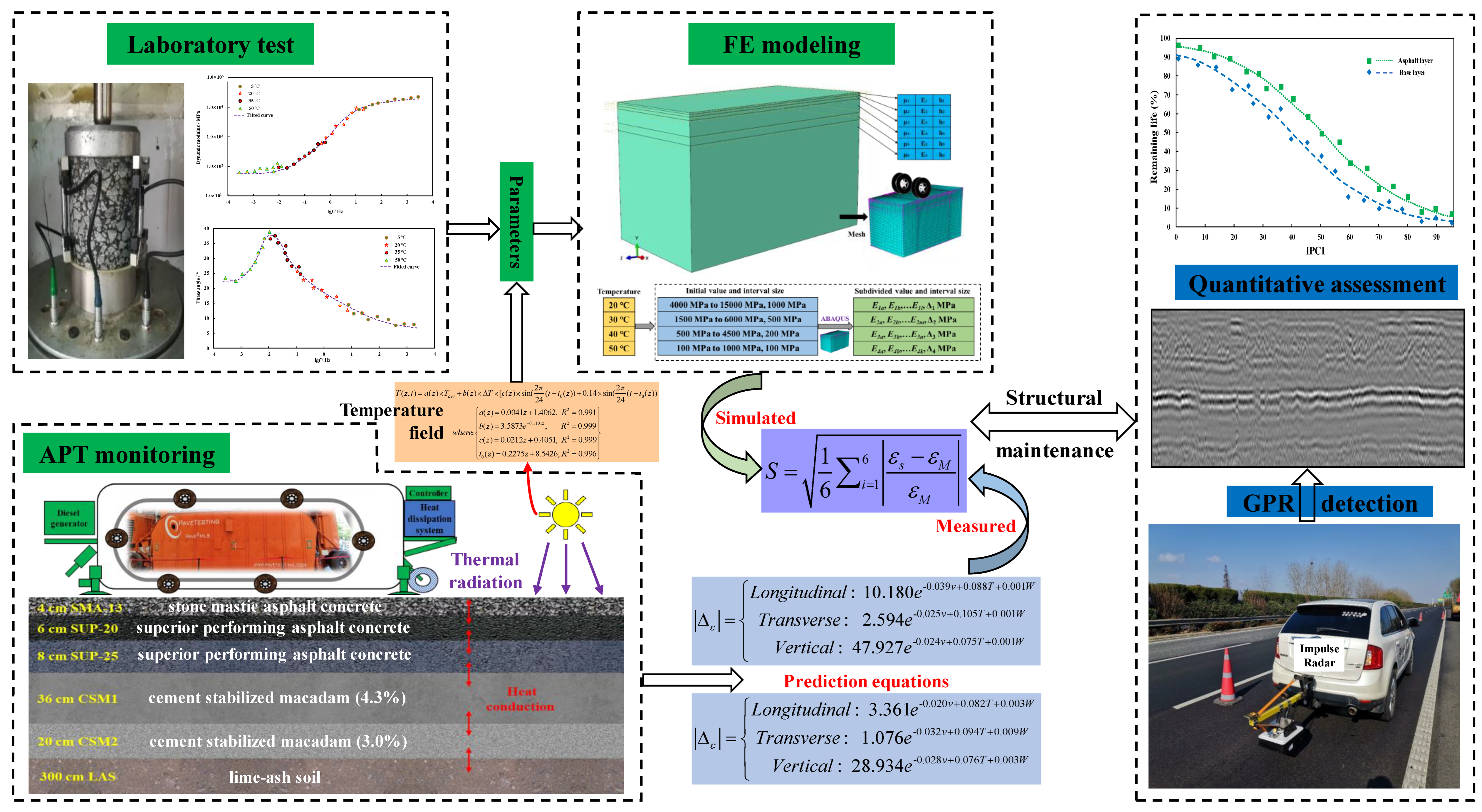
2. Materials and Method

As shown in Figure 1, the representative combination form of asphalt surface of Jiangsu expressway is “SMA-13 + SUP-20 + SUP-25”. Specifically, the material of the base layer is mainly crack-resistant cement-stabilized macadam (CSM), with a thickness of 36 cm to 40 cm. Therefore, the structure of the tested road in Zhenjiang, Jiangsu province was determined. The research procedure consisted of the following steps.

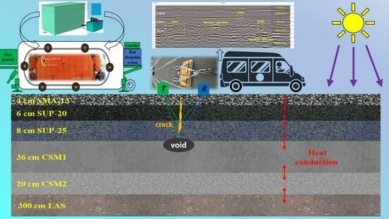
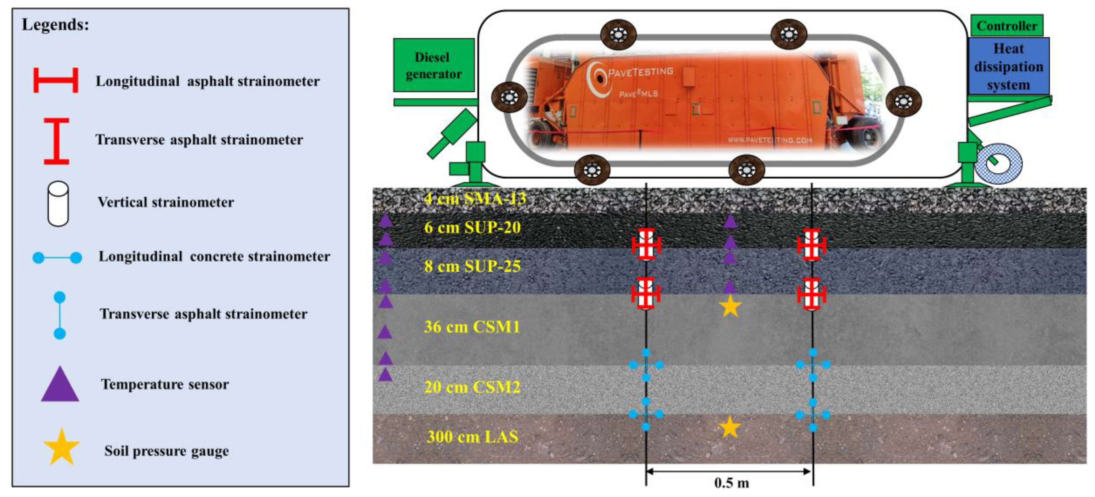
2.1. Field Investigation

2.1.1. Dynamic Modulus Tests

According to the test standard (JTG E20−2011) [40], the test temperature was divided into 5 °C, 20 °C, 35 °C, and 50 °C. The dimensions of the core samples (cylindrical shapes) of the asphalt layer were 100 mm × 100 mm × 150 mm. The specimens were stored in the thermostat for 4 to 5 h at each temperature grade. The specimens were installed and tested in UTM-25 equipment. To obtain the time spectrum representing the temperature dependence of asphalt mixtures, the test results were fitted according to the nonlinear least square method. The master curves of E* (20 °C) adhered to Equations (1)–(3) [41].
lg ( α T ) = C 1 ( T T s ) C 2 + T T s
where αT denotes the displacement factor, T denotes the test temperature, C1 and C2 represent the fitted parameters, and Ts denotes the reference temperature [42,43].
lg E = δ + α 1 + e β + γ lg ( f r )
lg ( f r ) = lg ( f ) + lg ( α T )
where f denotes testing frequency, fr represents the adjusted frequency, and αT, α, β, γ and δ are the regression constants, respectively.

2.1.2. Field Temperature Monitoring

The temperature of pavement structures at different depths z was collected from March 2020 to December 2020 using a resistive sensor with a frequency of 2 Hz. To eliminate the influence of noise on the testing results, the curves of temperature obtained by means of continuous collection were smoothed according to an interval of 10 min. According to the characteristic that the warming stage takes less time than the cooling stage, the hyperbolic sine function in Equation (4) was used to conduct regression analysis on the temperature field T(z, t) of asphalt pavement under different seasons (only non-rain weather was studied) and different depths.
T ( z , t ) = a × T a v e + b × Δ T × ( c × sin ( ω ( t t 0 ) ) + d × sin ( 2 ω ( t t 0 ) ) )
where Tave denotes the average of the maximum and minimum temperatures during one day, ΔT is the difference between them, ω is the angular frequency, t0 is the initial phase, and a, b, c, and d represent the regression coefficients.
After t0 was obtained by fitting the temperature under different months and depths, the regression analysis was performed again to obtain the initial phase t0 (z) at other z. Similarly, a and b were used to perform the regression analysis again after the first fitting to obtain the initial phase a (z) and b (z), respectively. After obtaining these regression relationships, the average values of a (z), b (z), c (z), and t0 (z) were obtained by means of different z fitting in each month and were functionally fitted with z as an independent variable, respectively.

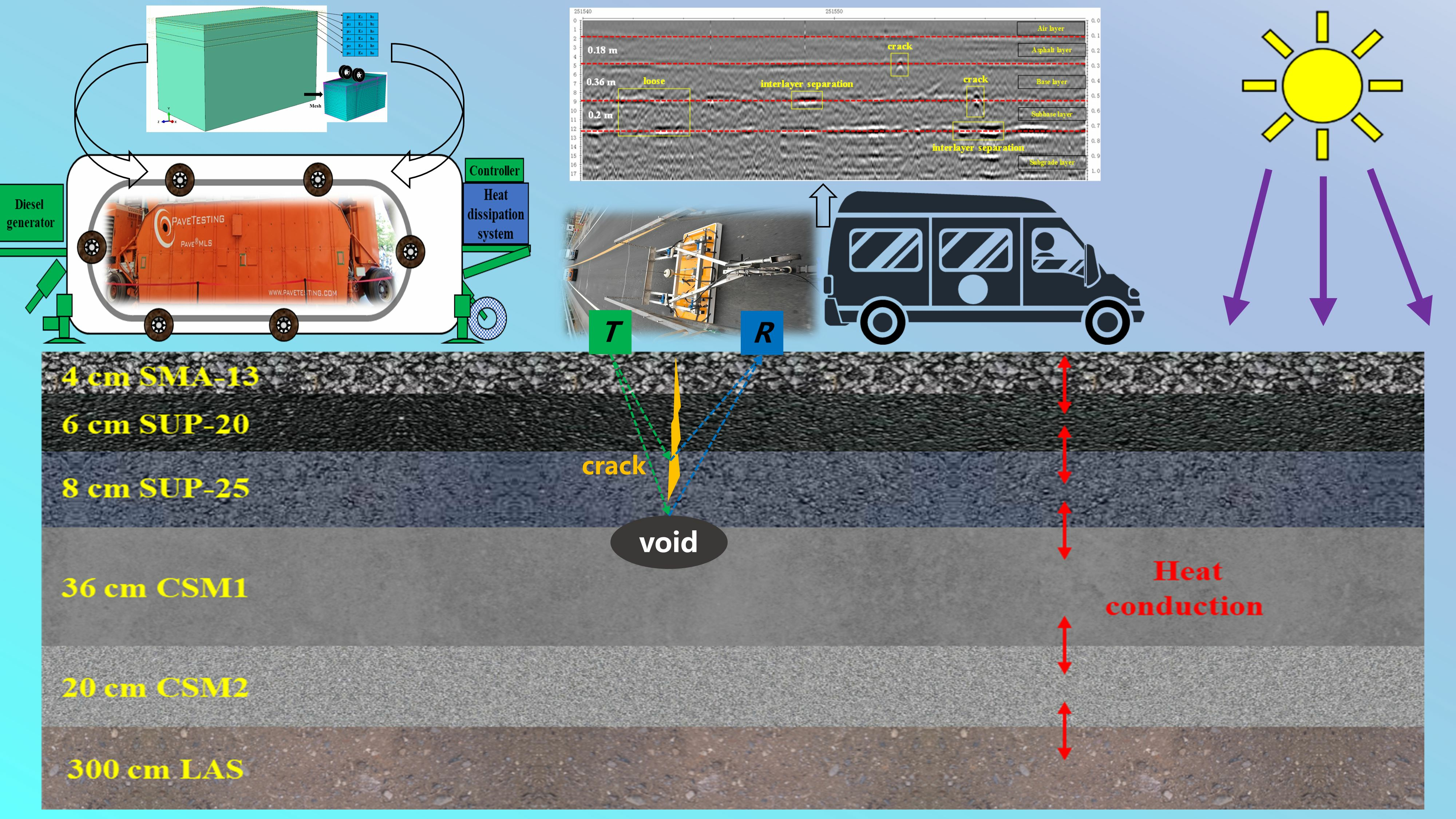
2.1.3. Accelerated Pavement Testing

As shown in Figure 2, the mobile load simulator (MLS66) equipment with internal twin-tires (305/70/R22.5) was performed to conduct the loading of the tested road under different temperature and speed conditions [42]. Figure 2 also depicts the cross-sectional layout scheme of monitoring sensors, considering the test coverage and sensor survival rate [44]. Temperature sensors were divided into two groups: one group was located in the middle and lower asphalt layers under the wheel track center for the purpose of monitoring temperature conditions, and the other group was situated on the edge of the road from the middle asphalt layer to the CMS2 layer for the purpose monitoring the natural temperature field of the road surface [45].
The strain sensors were all buried below the tire action point. The location of longitudinal, transverse, and vertical strain sensors was the same as that of the temperature sensors. At the bottom of the base layers, transverse and longitudinal horizontal-strain sensors were used [46].
Temperature (T), loading weight (W) and speed (v) were the three influencing factors [19]; thus, the loading scheme was as follows: 50, 60, and 75 kN for W; 10, 15, and 22 km/h for v; T: low (18 °C to 28 °C), middle (28 °C to 37 °C), and high temperatures (37 °C to 48 °C) for T. Then, the strain-temperature coefficient εT was defined in Equation (5) to calculate the strain transformation corresponding to the change in unit temperature [47].
ε T = ε 2 ε 1 T 2 T 1 ,
where T1 and T2 are the minimum and maximum values of the temperature range, and ε1 and ε2 are the corresponding strains, respectively. Combined with the measured strain values, the prediction equation of the strain amplitude (three-way: lateral, longitudinal, and vertical) ε for the bottom of the measured layers is described in Equation (6) [42].
| Δ ε | = a × e b × v + c × T + d × W ,
where a, b, c, and d denote the fitted parameters.

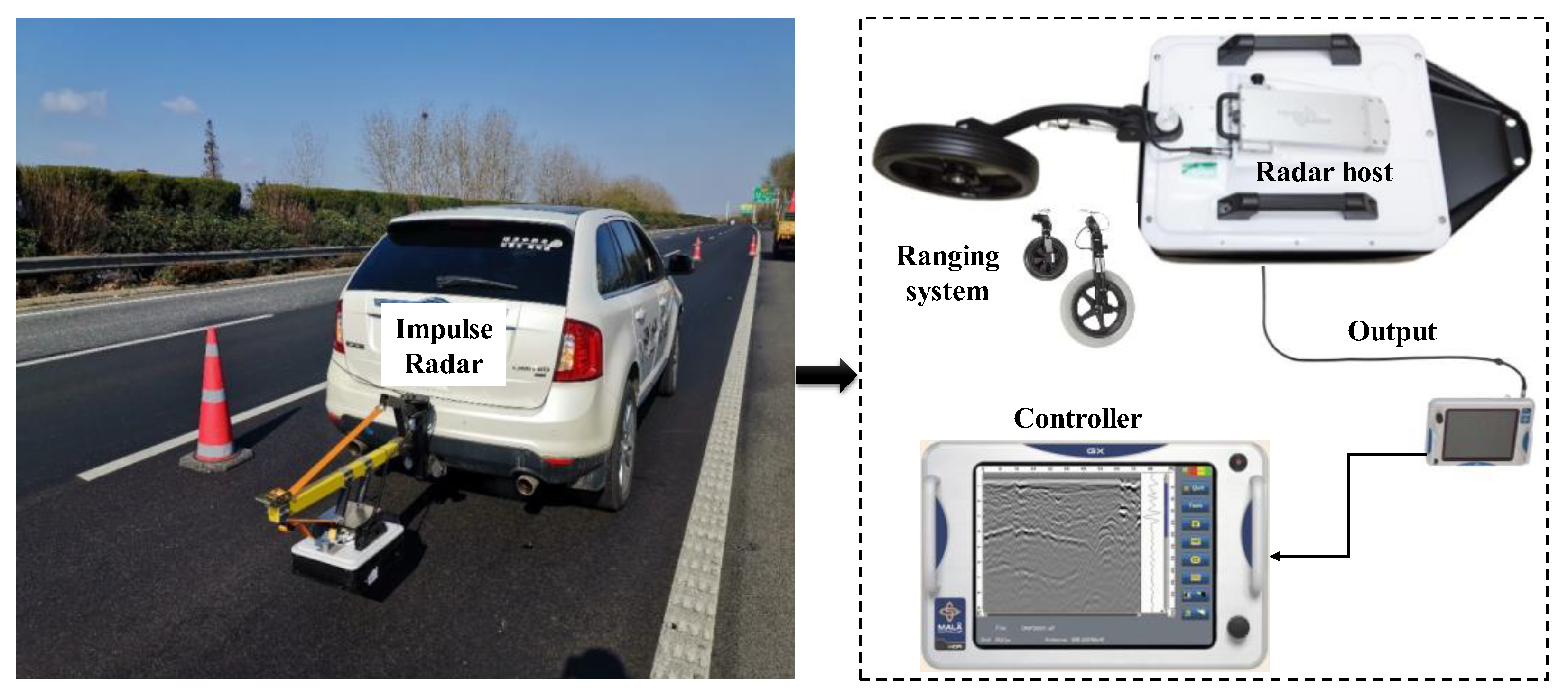
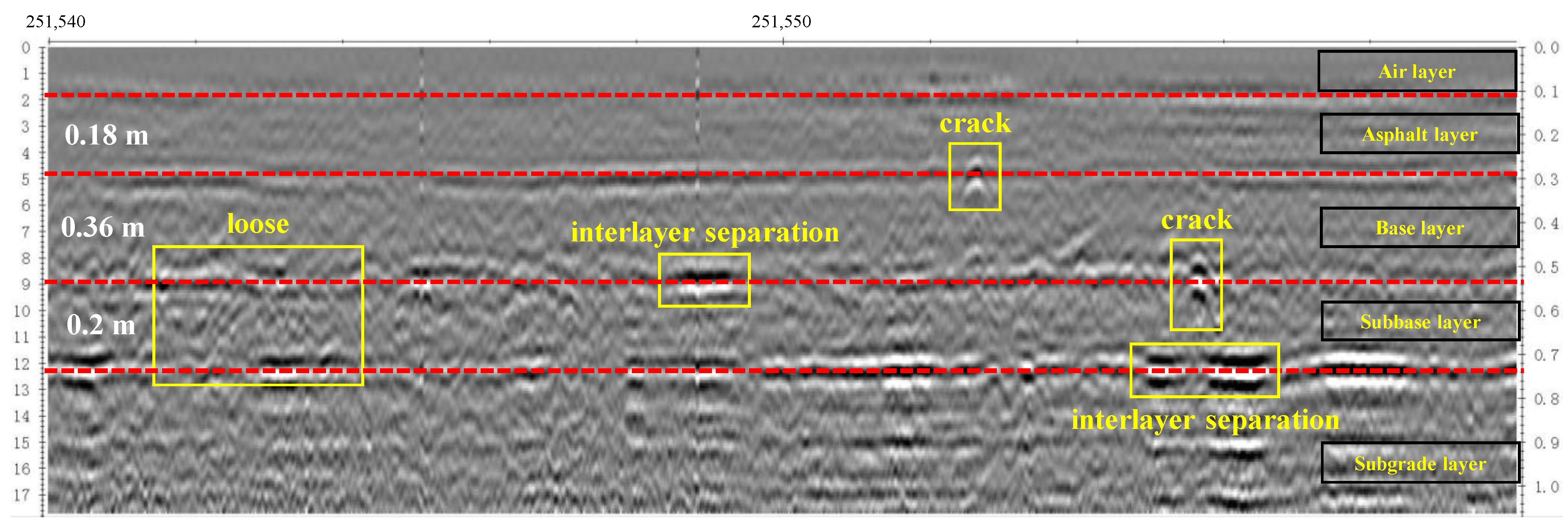
2.1.4. GPR Investigation

GPR investigation was performed on the road site with the same pavement structures in Figure 1 for its structural condition assessment. The detection equipment used was CO4080 vehicle-mounted GPR produced by Swedish Impulse, as shown in Figure 3. It is generally believed that the wheel track of the road is the most heavily loaded, and the structure of the wheel track can represent the internal condition of the overall road structure. Therefore, when selecting the vehicle-mounted GPR for the road survey, the measuring line should be situated on the wheel track of each lane. The detection parameter settings used by this GPR are shown in Table 1.
The distress characteristics were identified through GPR detection images of the longitudinal section of the road, according to the judgment results in previous studies [32,33,34,35,48]. In this study, the three most prevalent distresses were detected in this road section: cracks, looseness, and interlayer separation (IS). Then, the internal pavement condition index (IPCI) was used to evaluate the integrity of different structural layers of pavement, as shown in Equation (7).
I P C I = 100 i = 1 n S i S 0 × 100 % ,
where Si refers to the area of the ith distress (crack, looseness, and interlayer separation) in a structural layer (m2). S0 represent the area of the asphalt layer (0.18 × 100 = 18 m2) or the base layer (0.36 × 100 = 36 m2), as shown in Figure 4. In this study, only the structural conditions of asphalt surface and CSM base layers were analyzed. GPR investigation was performed for several sections of road on the G15 expressway of Jiangsu province, China, with different service lives. The length of the test road was 5 km, and the pavement structure was the same as in Figure 1. The IPCI index of the structural layers per 100 m of each road section was calculated to analyze the relationship between it and the remaining life of the structural layers.
Through the investigation and statistical analysis of typical pavement structure maintenance projects in Jiangsu Province, the overhaul cycle of the semi-rigid base pavement structure under different traffic conditions was obtained according to previous studies [49,50], as shown in Table 2. The traffic grade was divided according to the cumulative number of Ne (million times) of a single lane under the standard axle load (100 kN). Then, the remaining life ratio (RLR, %) was taken as an evaluation index, which represented the ratio of the service life of existing pavement to the upper service life limit of newly built pavement.
Thus, the RLR index of the structure in each maintenance stage could be calculated by comparing the findings of capital repair cycle and the partial repair cycle with the pavement service life, respectively, under various operating conditions.

2.2. Numerical Simulation

2.2.1. FE Modelling

The FE simulations of the field APT monitoring were performed using ABAQUS 2016 software to investigate the distribution state of dynamic responses under moving loads. Structural parameters of the asphalt surface were inverted, and the key mechanical response indexes were analyzed. In the FE model of the tested road, the X-axis was the lateral direction of the pavement, the Y-axis was the vehicle driving direction, and the Z-axis was the pavement layer depth direction, with lengths of 6 m, 10 m and 3.74 m, respectively.
The fixed constraint was chosen in the model (U1 = U2 = U3 = 0). The displacement in the Z-direction (U3 = 0) and X-direction was limited (U1 = 0), respectively [51]. Considering computing accuracy and efficiency, the mesh density of the surface layer and the grid near the loading area was improved. From the surface layer and the part of the load to the edge of the road, the grid was gradually thinned by means of the principle of equal difference distribution. The model mesh was divided using C3D8R (a three-dimensional eight-node hexahedral element with a linear reduction integral isoperimetric).
In addition, the load was 100 kN, the grounding pressure was 0.4456 MPa, and the action area was 0.035712 m2 (18.6 cm × 19.2 cm) in this FE model.

2.2.2. Viscoelastic Parameters

Based on the resting results of E*, the viscoelastic parameters were obtained using Prony series. The detailed steps in this process were as follows.
First, E* was converted to the relaxation modulus E(t). The first step was to calculate the storage modulus E’(f) at each frequency using Equation (8).
E ( f ) = E cos ( φ ) ,
where φ is the phase angle. The second step was to calculate log(f) of each frequency and perform a differential solution of lg(f) to calculate the slope n using Equation (9).
n = d lg E ( f ) d lg ( f ) ,
The third step was to calculate the adjustment function λ’ using Equation (10).
λ = Γ ( 1 n ) cos ( n π 2 ) w h e r e : Γ ( s ) = 0 + x s 1 e x d x ,   s 0 ,
The fourth step was to calculate E(t) using Equation (11).
E ( t ) = E ( f ) λ ,
Then, the master curve of E(t) was fitted. Subsequently, the shear modulus G(t) and its ratio g(t) were calculated by using Equations (12) and (13), respectively.
G ( t ) = E ( t ) 2 ( 1 + μ ) ,
G ( 0 ) = E ( 0 ) 2 ( 1 + μ ) = E ( t ) 2 ( 1 + μ ) = G ( t ) g ( t ) = G ( t ) / G 0 ,
Finally, Equation (14) was used to obtain the Prony series of asphalt mixtures.
g ( t ) = 1 i = 1 n g i ( 1 e ( t / τ i ) ) ,
where gi is the material constant, n is the number of items, and τi is the delay time [42].
Considering that the load capacity of the base, subbase, and subgrade layers was always stable during the loading process, these three layers were all taken as linear elastic materials in the FE model. The median value of the inverse modulus based on the FWD test was rounded as the elastic parameters of these three layers.

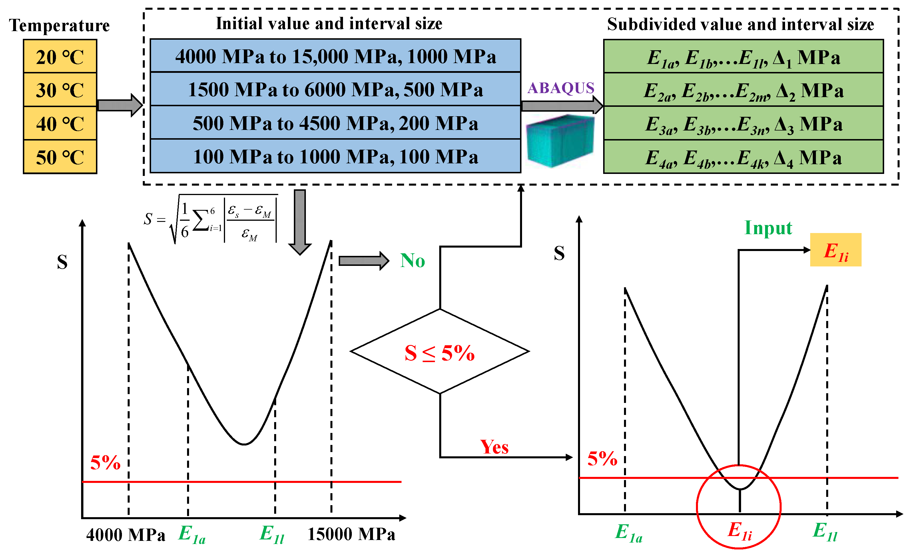
2.2.3. Material Parameter Inversion

Based on the response data measured on the tested road, the dynamic modulus values under different working conditions were inverted using ABAQUS 2016 software. The master curve of E* based on the measured dynamic responses was established and compared with that obtained from laboratory tests to achieve the E* correction of the asphalt layer.
First, monitoring response data of tested road were obtained according to Equation (6) under different working conditions, including four different loading temperatures (20 °C, 30 °C, 40 °C, and 50 °C) and three different loading speeds under an axial load of 50 kN. The calculated response data were the three-way strain of two measured layers (six data types).
As described in Figure 5, the varying ranges of the modulus of the asphalt surface in the FM model at different temperatures were set with the interval values of 1000 MPa, 500 MPa, 200 MPa, and 100 MPa, respectively, based on the test results of the dynamic modulus at different temperatures in Section 3.2.1. For each modulus value, six types of response peaks at different speeds were obtained by means of FE simulation, and the error S between the simulated strains εs and the measured strains εM was obtained according to Equation (15).
S = 1 6 i = 1 6 ε s ε M ε M ,
If S ≤ 5%, the inverse modulus could be determined. Otherwise, smaller interval values were further divided in the modulus range with the most minor error. The FE simulation was repeated until the error requirement was met. Thus, the inversion modulus values under twelve working conditions were obtained.

2.2.4. Fatigue Life Indexes

According to the design standard (JTG F50-2017) [52], fatigue cracking and permanent deformation of the asphalt layer and fatigue cracking of the base layer should be controlled. The fatigue life of the asphalt layer Nf1 and base layer Nf2 was calculated via Equations (16) and (17), respectively.
N f 1 = 6.32 × 10 15.96 0.29 β k a k b k T 1 1 ( 1 ε a ) 3.97 ( 1 E a ) 1.58 ( V F A ) 2.72 ,
where ka denotes the adjusted coefficient of seasonally frozen ground, kb denotes the coefficient of fatigue loading modes, Ea represents a E* at 20 °C, VFA represents the saturation of asphalt mixtures, kT1 is the adjusted coefficient of temperature, and β is the reliability coefficient.
N f 2 = k a k T 2 1 10 a b σ t R S + k c 0.57 β ,
where kT2 denotes the adjusted temperature coefficient, σt denotes the tension stress at the base layer bottom, RS represents the tension strength at the base layer, kc denotes the field comprehensive correction factor, and a and b denote fitted parameters.
Based on the predicted results of Equation (6), some indicators cannot be obtained via the APT monitoring. Therefore, the maximum shear strain, maximum compression stress of asphalt layer, and tension stress of base layer were calculated by means of FE simulation. Meanwhile, the most adverse and favorable conditions were selected to determine the reference scope for the values of the critical mechanical responses.

3. Results and Discussion

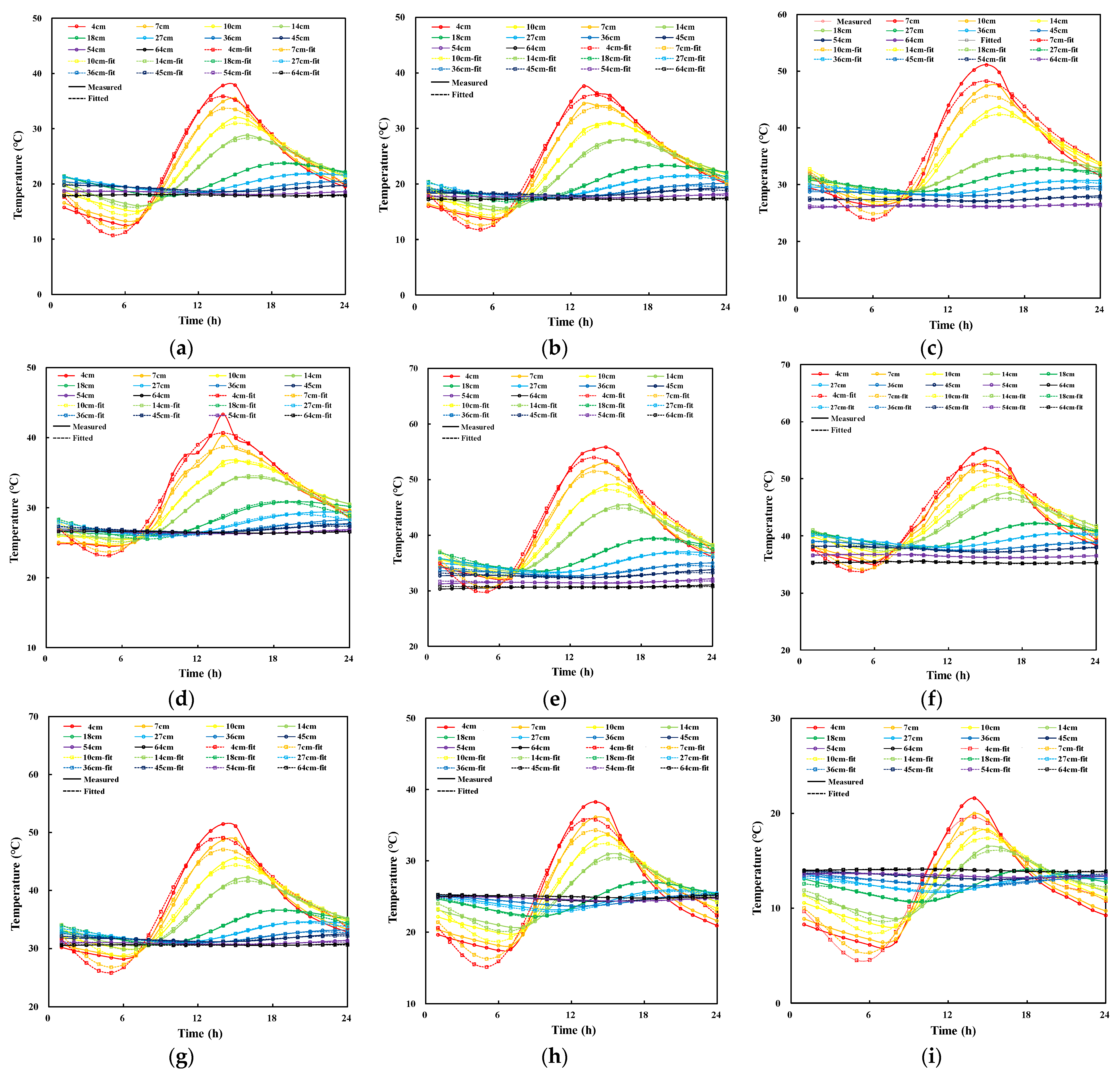
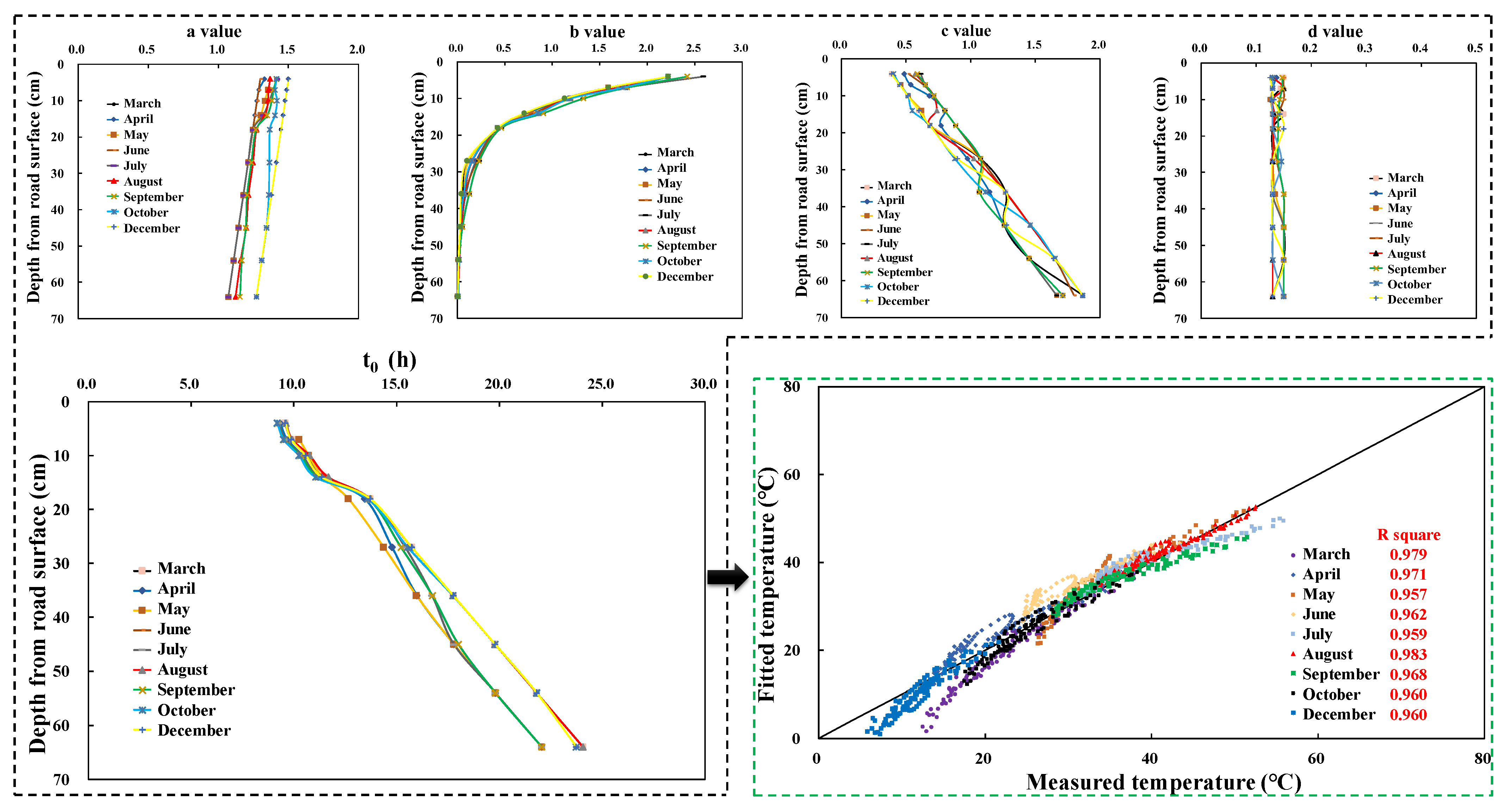
3.1. Field Temperature Monitoring

According to the measured temperature change curve of pavement structures along the z-direction, fitted results of the hyperbolic sine function in other representative months are shown in Figure 6.
The fitted results of a(z), b(z), c(z), and t0(z) are presented in Figure 7. Then, the temperature-field prediction model was obtained using Equation (18). The relationship between the measured and fitted temperatures was further explored. The correlation coefficient was above 0.95. This illustrates that the correlation was highly significant, which could predict the pavement structural temperatures.
T ( z , t ) = a ( z ) × T a v e + b ( z ) × Δ T × [ c ( z ) × sin ( 2 π 24 ( t t 0 ( z ) ) + 0.14 × sin ( 2 π 24 ( t t 0 ( z ) ) w h e r e a ( z ) = 0.0041 z + 1.4062 ,   R 2 = 0.991 b ( z ) = 3.5873 e 0.1101 z ,   R 2 = 0.999 c ( z ) = 0.0212 z + 0.4051 ,   R 2 = 0.999 t 0 ( z ) = 0.2275 z + 8.5426 ,   R 2 = 0.996 ,

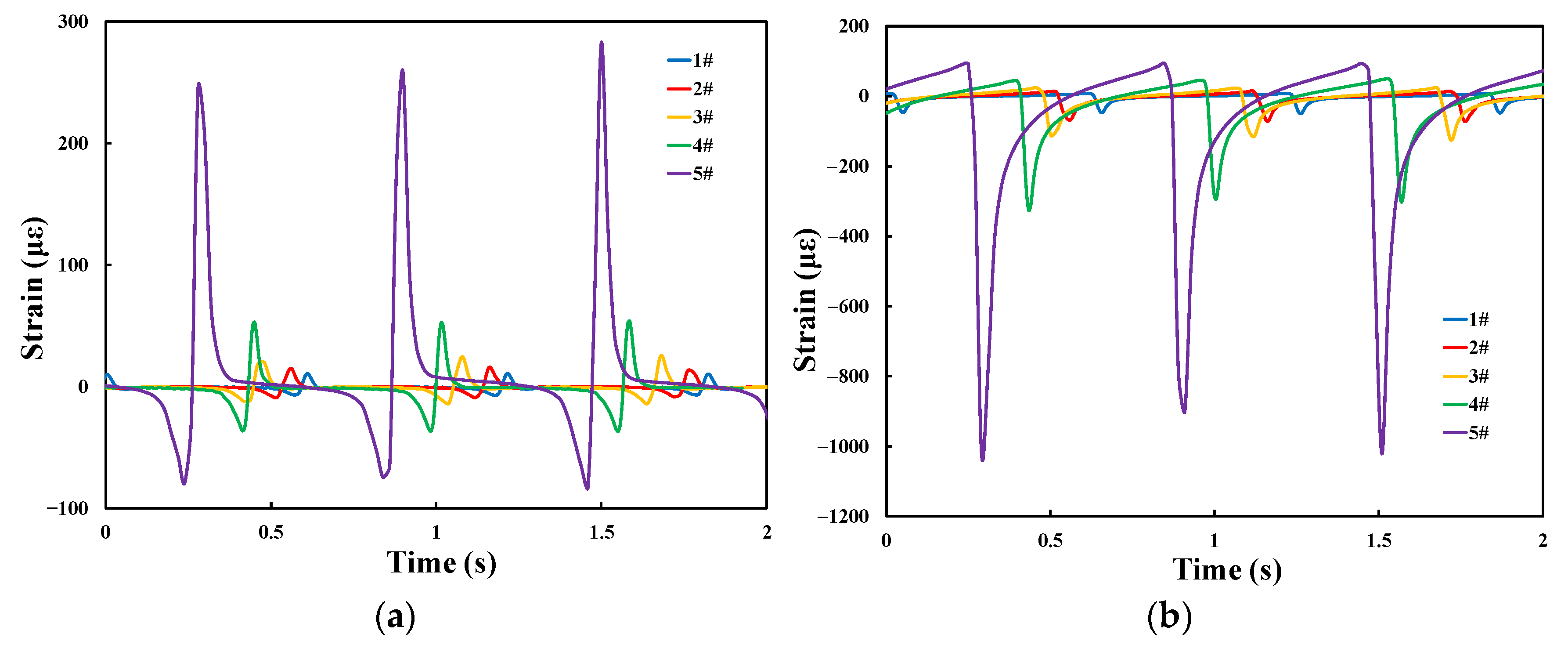
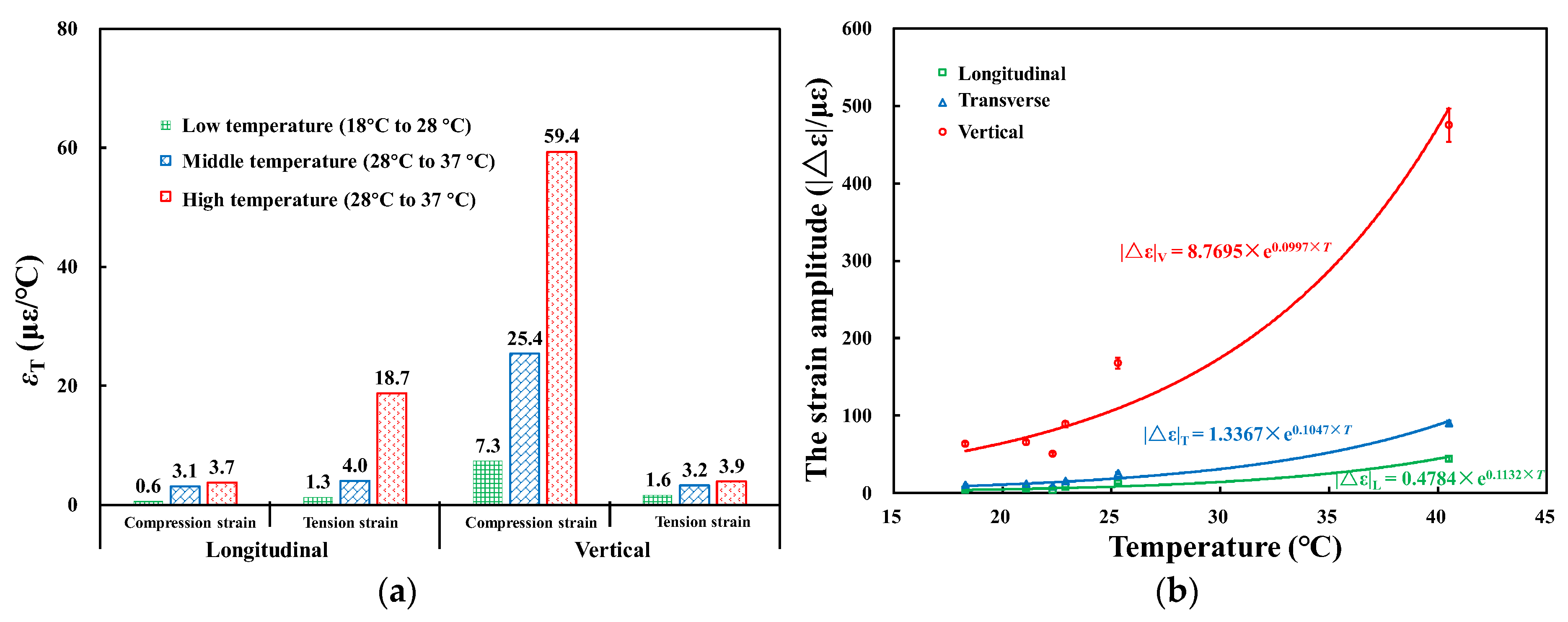
3.2. Dynamic Responses to Different Influencing Factors

In this section, the dynamic response to at different factors was analyzed, including the following points.

3.2.1. Field Temperature

The other two variables were a v of 22 km/h and a W of 50 kN. Figure 8 illustrates the measured strains at the bottom of the middle asphalt layer (z = 10 cm) at 1# to 5# temperature field. The peak strain increased with an increase in temperature. When the temperature was 47.9 °C (5# high-temperature field), the extreme values of longitudinal and vertical strains were 262.53 με and −979.70 με, 25.4 times and 21.6 times those of 18.9 °C, respectively. This shows that the strain at the bottom of the middle asphalt layer is greatly affected by the pavement temperature field.
Figure 9a further presents the calculation results of εT. This figure illustrates that the εT of vertical compression strain was the largest, indicating that it is most sensitive to temperature changes in different regions. Under the high-temperature condition, the vertical compression strain increased by 59.4 με for every 1 °C temperature increase, being 8.1 times that under the low-temperature condition. The second was the longitudinal tension-strain: it increased by 4.0 με and 18.7 με for each 1 °C increase in temperature under the middle- and high-temperature conditions, respectively. In addition, the longitudinal compression-strain and vertical tension-strain were little affected by temperature, and the εT was in the range of 1 to 4 με/°C under three temperature conditions.
Figure 9b displays the curve of three-way strain amplitude changing with temperature. The three-way strain amplitudes all showed positive exponential growth with temperature. The vertical strain amplitudes were larger than the transverse and longitudinal strain amplitudes under different temperature fields. The results are consistent with previous studies [17].

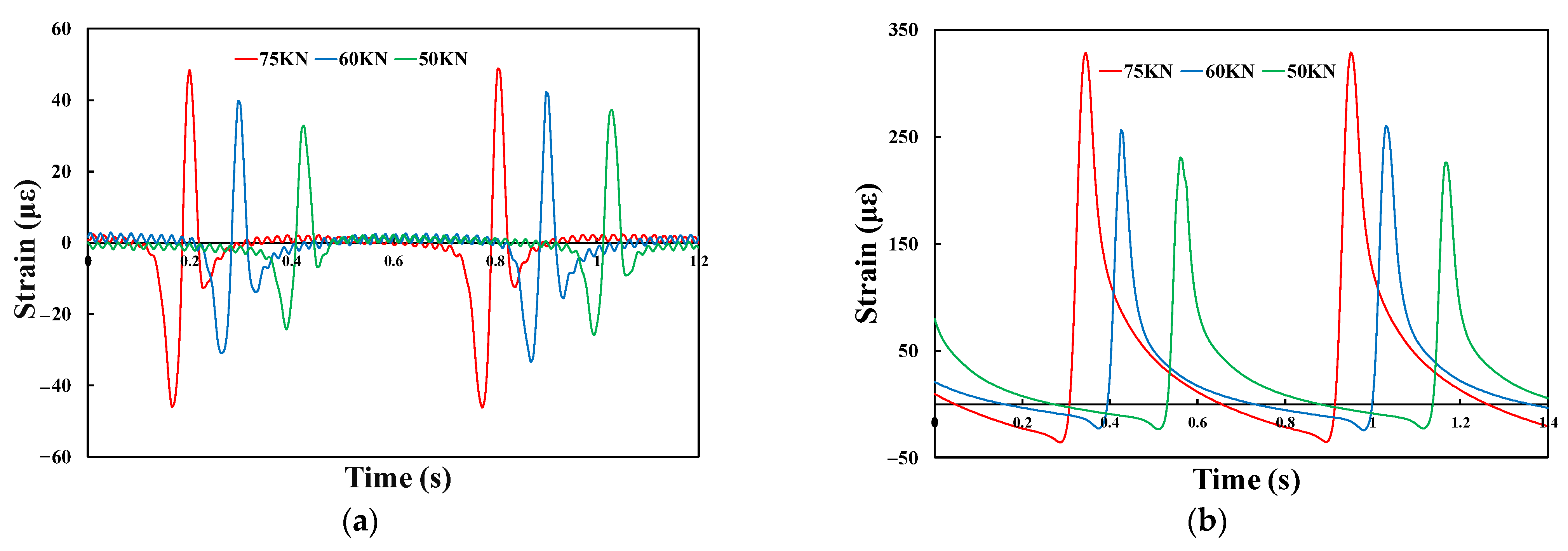
3.2.2. Loading Weight

The other variables were a T of 37 °C (bottom of middle asphalt layer bottom) and a v of 22 km/h. Figure 10 demonstrates the measured strain curves under different W. W is a critical influencing factor affecting pavement dynamic responses, and strain increases linearly with the change in the loading weight. Specifically, when W was 50 kN, the longitudinal and vertical strain amplitudes were 32.7 με and 230.2 με, respectively. When W was 60 kN, the longitudinal strain and vertical strain amplitudes were 38.6 με and 255.9 με, respectively, which increased by 18% and 11.2% compared with those of 50 kN and was further increased by 48% and 39.8% when W was 75 kN. This study’s relationship between loading weight and mechanical response agrees with earlier studies [53,54].

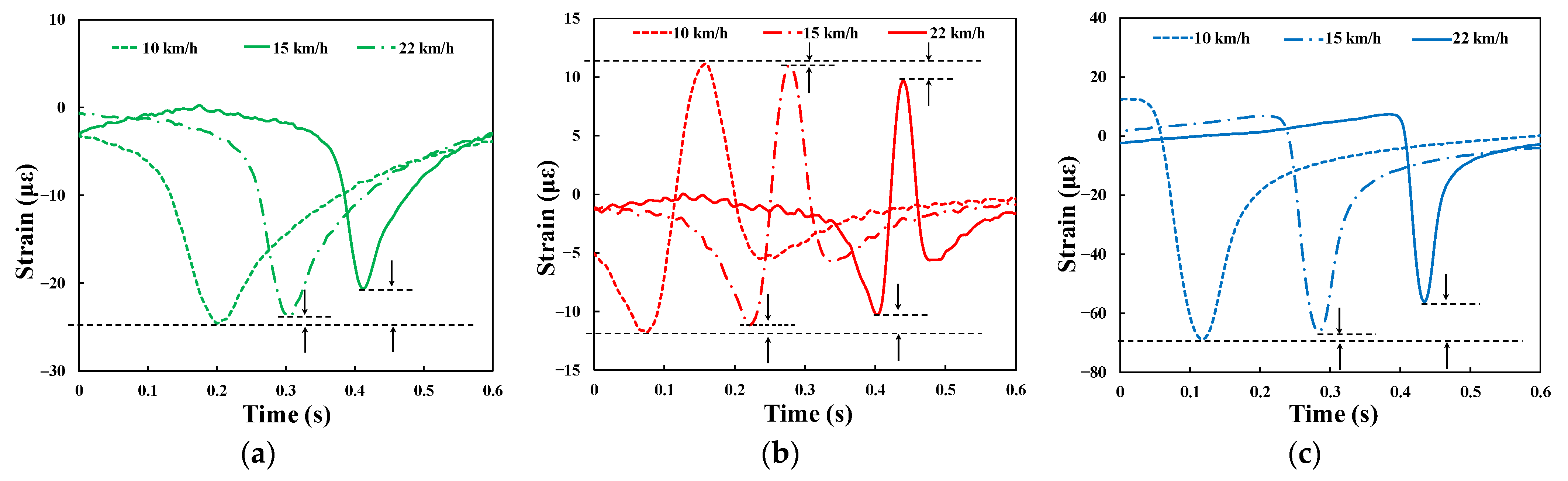
3.2.3. Loading Speed

The other two variables were a T of 37 °C (bottom of middle asphalt layer bottom) and a W of 50 kN. Three-way strain curves under different v are presented in Figure 11.
It can be seen that the three-way strain amplitudes were all at the maximum level when v = 10 km/h. Then, the amplitude decreased as v increased. With the decrease in loading speed, the frequency of loading rotation for asphalt mixture increases correspondingly, and the interaction time between the wheels and the road surface lengthens. As a result, both the action time and the amplitude for the time-course curve of strain in the pavement increased, which agrees with the results published in Refs. [55,56]. Therefore, the lower the speed in the pavement service process, the more extensive the three-way strain amplitude and high-strain area over time, resulting in fatigue cracking prematurely at the asphalt layer bottom.

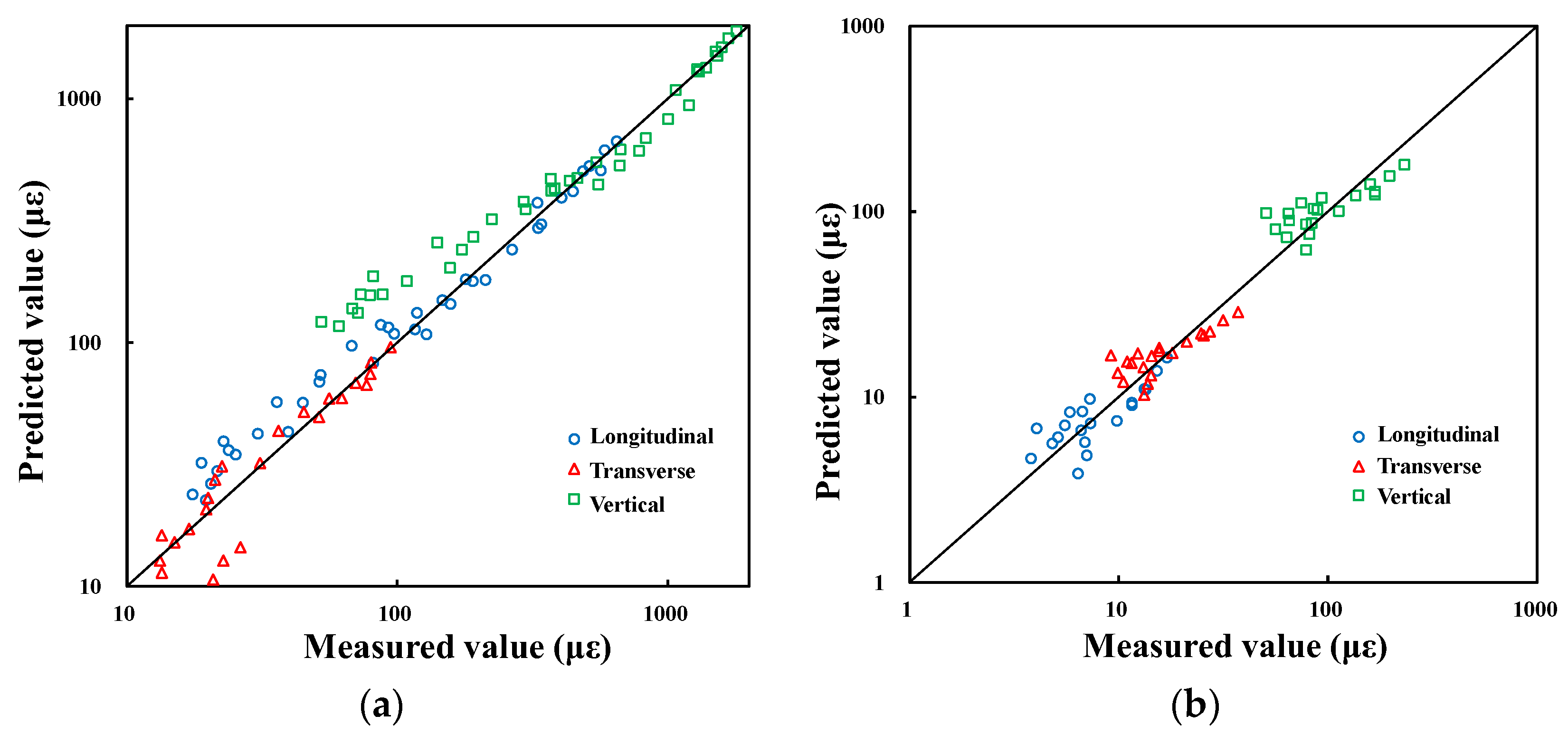
3.3. Dynamic Response Prediction

Following the above analysis from Section 3.2.1, Section 3.2.2 and Section 3.2.3, it was found that the measured strain amplitudes were positively correlated with temperatures and loading weights but negatively correlated with loading speeds. Combining Equation (6) with the measured data of the tested road, the prediction equations of three-way strain amplitude were developed under multiple factors, as shown in Equations (19) and (20), respectively.
Δ ε = L o n g i t u d i n a l :   10.180 e 0.039 v + 0.088 T + 0.001 W ,   R 2 = 0.99 T r a n s v e r s e : 2.594 e 0.025 v + 0.105 T + 0.001 W ,   R 2 = 0.98 V e r t i c a l :   47.927 e 0.024 v + 0.075 T + 0.001 W ,   R 2 = 0.99 ,
Δ ε = L o n g i t u d i n a l :   3.361 e 0.020 v + 0.082 T + 0.003 W ,   R 2 = 0.97 T r a n s v e r s e : 1.076 e 0.032 v + 0.094 T + 0.009 W ,   R 2 = 0.97 V e r t i c a l :   28.934 e 0.028 v + 0.076 T + 0.003 W ,   R 2 = 0.96
Figure 12 further describes the relationship between the monitoring and predicted data of three-way strain amplitude. It exhibits a good correlation, with all correlation coefficients being above 0.96, which is better than the values obtained by most previous studies [14,57].

3.4. Finite Element Simulation

In this section, the FE simulation results and their applications are discussed, including the following points.

3.4.1. Results of Material Parameter Inversion

Table 3 summarizes the calculated εM of the tested road according to Equations (19) and (20) under different working conditions, including the three-way strain at the bottom of the two measured layers.
Then, the modulus inversion was performed based on Figure 9. The calculated error (S) at the final iteration round and the modulus is summarized in Table 4.
The corresponding modulus of the minimum S (≤5%) was selected to obtain the optimal modulus of the asphalt layer at various working conditions (red font in Table 3). Therefore, its back-calculated modulus combining measured data and FE simulation was realized, which provided reliable parameter input for the subsequent simulation analysis of the key mechanical indexes.

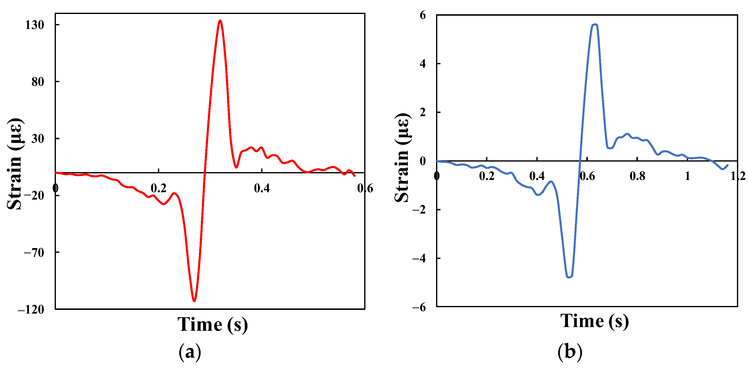
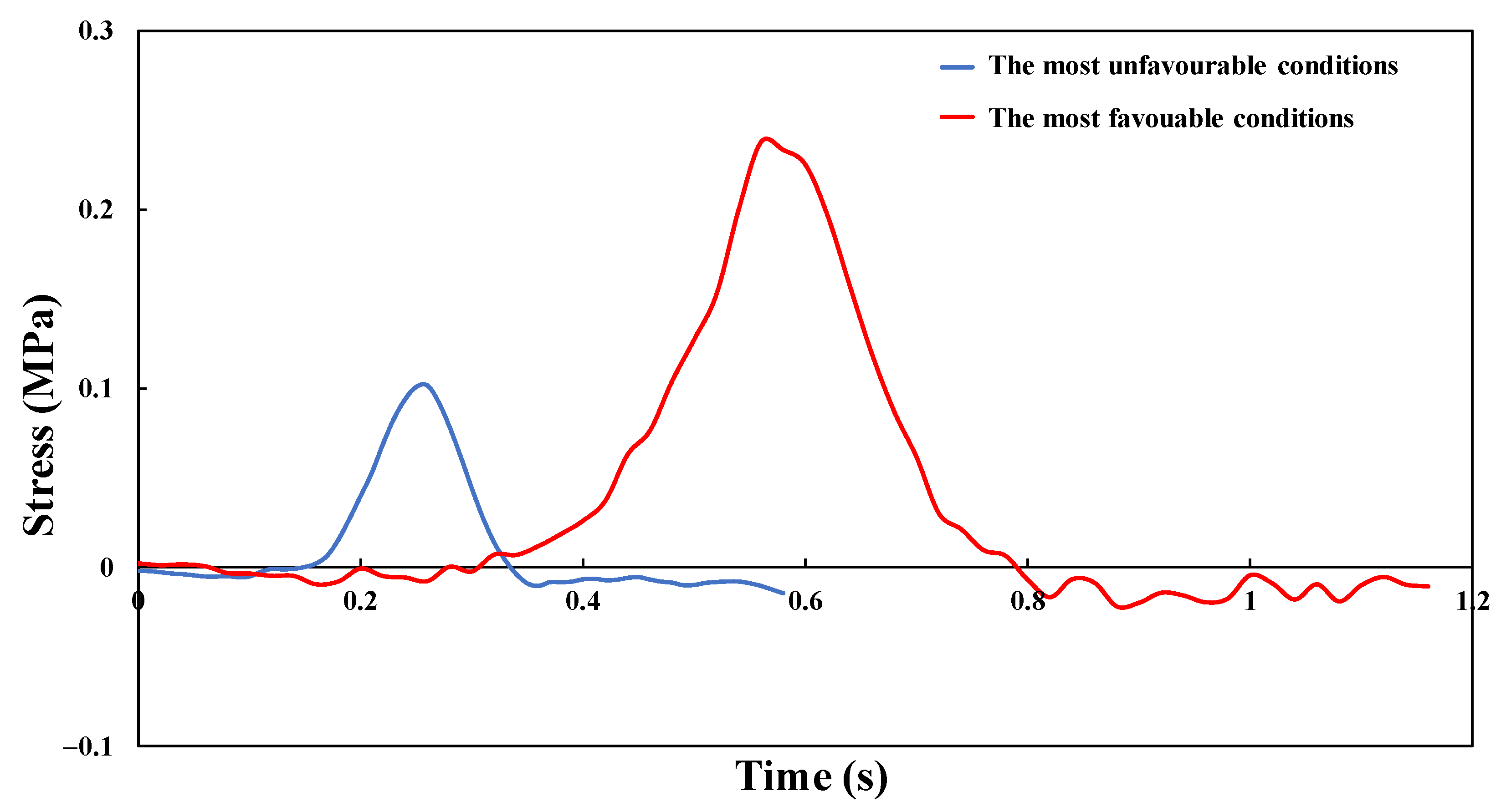
3.4.2. Prediction Results of Fatigue Failure and Critical Conditions

Based on the analysis results from Section 3.2 and Section 3.3, the mechanical indexes of the structural layers in the tested road increased nonlinearly with increasing T and W, and decreasing v. Combined with loading test conditions, it can be determined that the most unfavorable combination was 75 kN and 10 km/h at 5# temperature field. The most favorable combination was 50 kN and 22 km/h at 1# temperature field. According to Equation (20), the calculated tension and compression strains at the bottom of the asphalt layer were as follows: the maximum tension strain under the most unfavorable and favorable working conditions was 164.39 με and 5.44 με, respectively. The maximum compression strain under the most unfavorable and favorable working conditions was 1210.36 με and 82.73 με, respectively.
Combined with these results and Equation (16), it can be calculated that the Nf1 of the asphalt layer is between 2.24 × 10⁷ and 1.69 × 10¹³ equivalent-axle times. In the light of a previous study [41], the maximum shear strain of a typical structure occurred at the top of the middle surface layer (6 cm below the pavement), and the change rule of shear strain with time under the most unfavorable and favorable conditions was further simulated. Figure 13 suggests that the maximum shear strain of the asphalt layer of a semi-rigid pavement ranged from 5.53 με to 133.48 με.
The FE calculation results in Figure 14 demonstrate that the tension stress at the bottom of the base layer was between 0.101 MPa and 0.237 MPa under different working conditions. Combined with Equation (17), it could be calculated that the Nf2 of the base layer is between 5.33 × 10⁸ and 4.60 × 10¹⁰ equivalent-axle times.

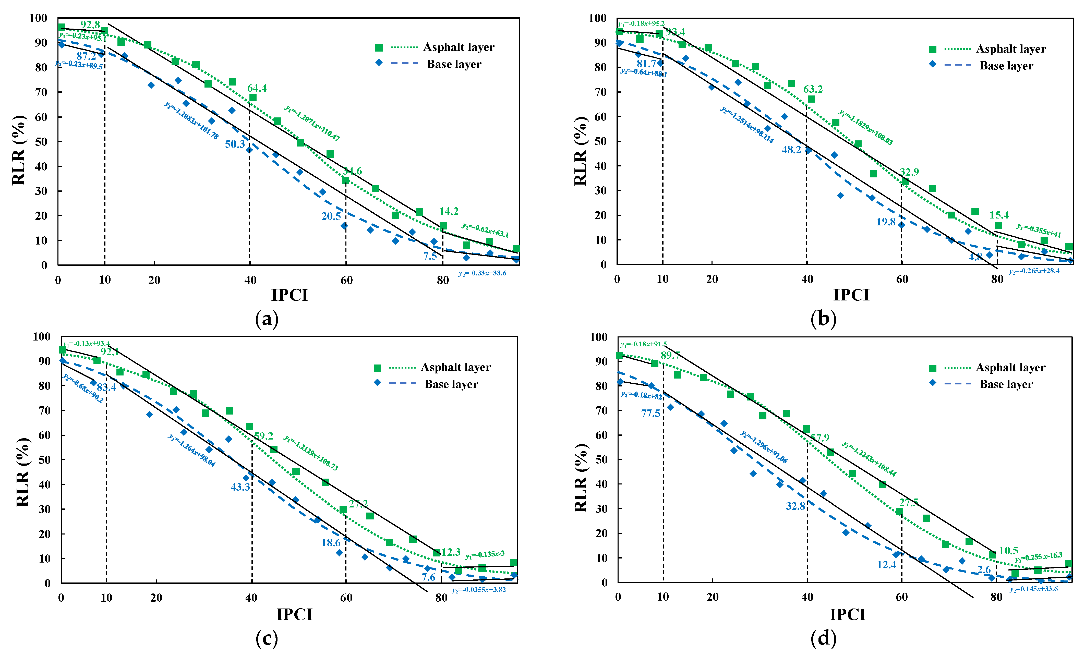
3.5. Relationship between Pavement Structural Conditions and Remaining Life

After GPR detection of several highways in Jiangsu Province, Figure 15 illustrates the relationship between the IPCI and RLR of the asphalt surface and CSM base layers under different traffic levels. The following points summarize our findings:
  • Linear fitting was performed for the data with IPCI less than 10, IPCI greater than 80 and the intermediate segment, respectively. IPCI and RLR showed a roughly negative relationship: when the IPCI was less than 10, the slope k of the line was small (about 0.2). It was significant larger when the IPCI was greater than 10 (between 1.1 to 1.3); however, it became small again after the IPCI was greater than 80.
  • With the increase in traffic grade, the IPCI of different structural layers decreased to different degrees, and the IPCI of the base layer decreased more obviously due to load accumulation. On the other hand, the fitting relationship between IPCI and RLR was slightly weakened, which may be because the thickness of pavement structural layers changes under repeated load, thus affecting the calculation result of IPCI.
  • Under the same IPCI value, the RLR of the base layer was lower than that of the asphalt surface layer, and this difference was more evident with the increase in traffic grade. This may be due to the increase in the distress ratio, as the performance of the CSM base material decreases significantly, and the modulus attenuation is greater.

4. Conclusions

This study assesses structural conditions and remaining life by combining APT and GPR for semi-rigid base pavement. The main conclusions are as follows:
(1)
Temperatures were predicted using a dual sinusoidal model for pavement structures based on the measured atmospheric temperature and structural temperatures. The good linear correlation (coefficient > 0.95) indicates that this model is reliable.
(2)
The asphalt surface layer showed a three-way strain increase with increasing temperature and load weight, but a decrease with increasing loading speed. It was excellently correlated with the measured values to predict dynamic responses under multivariate factors.
(3)
The material parameter inversion of the asphalt surface layer was proposed by controlling the average error of six strains between the FE-simulated and APT-measured values. Based on the established FE model, key mechanical index values can be analyzed under different conditions, along with the fatigue life of pavement structural layers.
(4)
There is a good negative correlation between the IPCI and the RLR of the pavement structure. Therefore, the RLR of the pavement structure can be predicted via GPR detection and quantitative assessment of structure conditions.
This work solves the problems of assessing the condition of pavement structures quantitatively that could guide asphalt pavement maintenance with a semi-rigid base. It is worth noting that the asphalt surface layer is only studied as a whole because the material parameters are obtained via indoor testing of the specimens with on-site coring in the tested road. In addition, fluctuating loads are also an important factor. Future research could establish a finite element model of pavement structure considering load fluctuation and modify it with APT-measured data.

Author Contributions

The authors confirm contributions to the paper as follows: study conception and design: Z.L.; data collection: Z.L. and Q.Y.; analysis and interpretation of results: Z.L. and Q.Y.; draft manuscript preparation: Z.L., Q.Y. and X.G. All authors have read and agreed to the published version of the manuscript.

Funding

This research received no external funding.

Data Availability Statement

Restrictions apply to the availability of these data. Data can be obtained from the corresponding author upon request.

Conflicts of Interest

The authors declare no conflict of interest.

References

  1. Wang, D.; Liu, Z.; Gu, X.; Wu, W.; Chen, Y.; Wang, L. Automatic Detection of Pothole Distress in Asphalt Pavement Using Improved Convolutional Neural Networks. Remote Sens. 2022, 14, 3892. [Google Scholar] [CrossRef]
  2. Ren, D.Y.; Song, H.; Huang, C.; Xiao, C.; Ai, C.F. Comparative Evaluation of Asphalt Pavement Dynamic Response with Different Bases under Moving Vehicular Loading. J. Test. Eval. 2020, 48, 1823–1836. [Google Scholar] [CrossRef]
  3. Liu, Z.; Gu, X.Y.; Ren, H.; Wang, X.; Dong, Q. Three-dimensional finite element analysis for structural parameters of asphalt pavement: A combined laboratory and field accelerated testing approach. Case Stud. Constr. Mat. 2022, 17, e01221. [Google Scholar] [CrossRef]
  4. Liu, Z.; Gu, X.; Ren, H. Rutting prediction of asphalt pavement with semi-rigid base: Numerical modeling on laboratory to accelerated pavement testing. Constr. Build. Mater. 2023, 375, 130903. [Google Scholar] [CrossRef]
  5. Ingrassia, L.P.; Virgili, A.; Canestrari, F. Effect of geocomposite reinforcement on the performance of thin asphalt pavements: Accelerated pavement testing and laboratory analysis. Case Stud. Constr. Mat. 2020, 12, e00342. [Google Scholar] [CrossRef]
  6. Al-Qadi, I.L.; Loulizi, A.; Elseifi, M.; Lahouar, S. The Virginia Smart Road: The impact of pavement instrumentation on understanding pavement performance. J. Assoc. Asph. Pavement 2004, 73, 427–465. [Google Scholar]
  7. Dessouky, S.H.; Alqadi, I.L.; Yoo, P.J. Full-Depth Flexible Pavement Response to Different Truck Tire Loadings. In Proceedings of the Transportation Research Board Meeting, Washington, DC, USA, 21–25 January 2007. [Google Scholar]
  8. Bhattacharjee, S.; Mallick, R.B. Effect of temperature on fatigue performance of hot mix asphalt tested under model mobile load simulator. Int. J. Pavement Eng. 2012, 13, 166–180. [Google Scholar] [CrossRef]
  9. Han, Z.; Sha, A.; Hu, L.; Jiao, L. Modeling to simulate inverted asphalt pavement testing: An emphasis on cracks in the semirigid subbase. Constr. Build. Mater. 2021, 306, 124790. [Google Scholar] [CrossRef]
  10. Zhu, X.Y.; Zhang, Q.F.; Chen, L.; Du, Z. Mechanical response of hydronic asphalt pavement under temperature-vehicle coupled load: A finite element simulation and accelerated pavement testing study. Constr. Build. Mater. 2021, 272, 121884. [Google Scholar] [CrossRef]
  11. Greene, J.; Choubane, B.; Upshaw, P. Evaluation of a Heavy Polymer Modified Asphalt Binder Using Accelerated Pavement Testing. In Proceedings of the 4th International Conference on Accelerated Pavement Testing, Davis, CA, USA, 19–21 September 2012. [Google Scholar]
  12. Blab, R.; Kluger-Eigl, W.; Füssl, J.; Arraigada, M.; Hofko, B. Accelerated Pavement Testing on Slab and Block Pavements using the New Mobile Load Simulator MLS10. In Proceedings of the 4th International Conference on Accelerated Pavement Testing, Davis, CA, USA, 19–21 September 2012. [Google Scholar]
  13. Jansen, D.; Wacker, B.; Pinkofsky, L. Full-scale accelerated pavement testing with the MLS30 on innovative testing infrastructures. Int. J. Pavement Eng. 2018, 19, 456–465. [Google Scholar] [CrossRef]
  14. Zhang, H.; Ren, J.; Ji, L.; Wang, L. Mechanical response measurement and simulation of full scale asphalt pavement. J. Harbin Inst. Technol. 2016, 48, 41–48. [Google Scholar]
  15. Zaumanis, M.; Haritonovs, V. Long term monitoring of full scale pavement test section with eight different asphalt wearing courses. Mater. Struct. 2016, 49, 1817–1828. [Google Scholar] [CrossRef]
  16. Liu, Z.; Gu, X. Performance Evaluation of Full-scale Accelerated Pavement using NDT and Laboratory Tests: A case study in Jiangsu, China. Case Stud. Constr. Mat. 2023, 18, e02083. [Google Scholar] [CrossRef]
  17. Ling, J.M.; Wei, F.L.; Zhao, H.D.; Tian, Y.; Han, B.Y.; Chen, Z.A. Analysis of airfield composite pavement responses using full-scale accelerated pavement testing and finite element method. Constr. Build. Mater. 2019, 212, 596–606. [Google Scholar] [CrossRef]
  18. Yang, H.L.; Wang, S.J.; Miao, Y.H.; Wang, L.B.; Sun, F.Y. Effects of accelerated loading on the stress response and rutting of pavements. J. Zhejiang Univ. Sci. A 2021, 22, 514–527. [Google Scholar] [CrossRef]
  19. Ai, C.F.; Rahman, A.; Xiao, C.; Yang, E.H.; Qiu, Y.J. Analysis of measured strain response of asphalt pavements and relevant prediction models. Int. J. Pavement Eng. 2017, 18, 1089–1097. [Google Scholar] [CrossRef]
  20. Chun, S.; Kim, K.; Greene, J.; Choubane, B. Evaluation of interlayer bonding condition on structural response characteristics of asphalt pavement using finite element analysis and full-scale field tests. Constr. Build. Mater. 2015, 96, 307–318. [Google Scholar] [CrossRef]
  21. Ma, X.; Dong, Z.; Chen, F.; Xiang, H.; Cao, C.; Sun, J. Airport asphalt pavement health monitoring system for mechanical model updating and distress evaluation under realistic random aircraft loads. Constr. Build. Mater. 2019, 226, 227–237. [Google Scholar] [CrossRef]
  22. Li, N.; Zhan, H.; Yu, X.; Tang, W.; Yu, H.; Dong, F. Research on the high temperature performance of asphalt pavement based on field cores with different rutting development levels. Mater. Struct. 2021, 54, 70. [Google Scholar] [CrossRef]
  23. Gouveia, B.C.S.; Preti, F.; Cattani, L.; Bozzoli, F.; Roberto, A.; Romeo, E.; Tebaldi, G. Numerical and Experimental Analysis of the Raise-Temperature Effect of Quicklime in Cold Recycled Mixtures. J. Mater. Civil. Eng. 2022, 34, 04022283. [Google Scholar] [CrossRef]
  24. Liu, Z.; Gu, X.; Dong, X.; Cui, B.; Hu, D. Mechanism and Performance of Graphene Modified Asphalt: An Experimental Approach Combined with Molecular Dynamic Simulations. Case Stud. Constr. Mat. 2022, 18, e01749. [Google Scholar] [CrossRef]
  25. Liu, Z.; Sun, L.; Gu, X.; Wang, X.; Dong, Q.; Zhou, Z.; Tang, J. Characteristics, mechanisms, and environmental LCA of WMA containing sasobit: An analysis perspective combing viscosity-temperature regression and interface bonding strength. J. Clean. Prod. 2023, 391, 136255. [Google Scholar] [CrossRef]
  26. Yang, J.; Fang, Y. Rationality and Applicability of High-Temperature Performance Indexes for Polymer-Modified Asphalts. J. Mater. Civ. Eng. 2021, 33, 04021238. [Google Scholar] [CrossRef]
  27. Barber, E.S. Calculation of Maximum Pavement Temperatures from Weather Reports. Highw. Res. Board Bull. 1957, 168. Available online: http://onlinepubs.trb.org/Onlinepubs/hrbbulletin/168/168-001.pdf (accessed on 29 June 2023).
  28. Anupam, K.; Srirangam, S.K.; Scarpas, A.; Kasbergen, C. Influence of Temperature on Tire-Pavement Friction: Analyses. Transp. Res. Rec. 2013, 2369, 114–124. [Google Scholar] [CrossRef]
  29. Si, W.; Ma, B.; Ren, J.P.; Hu, Y.P.; Zhou, X.Y.; Tian, Y.X.; Li, Y. Temperature responses of asphalt pavement structure constructed with phase change material by applying finite element method. Constr. Build. Mater. 2020, 244, 118088. [Google Scholar] [CrossRef]
  30. Zhao, X.Y.; Shen, A.Q.; Ma, B.F. Temperature response of asphalt pavement to low temperatures and large temperature differences. Int. J. Pavement Eng. 2020, 21, 49–62. [Google Scholar] [CrossRef]
  31. Luo, X.; Gu, F.; Lytton, R.L. Kinetics-based aging prediction of asphalt mixtures using field deflection data. Int. J. Pavement Eng. 2019, 20, 287–297. [Google Scholar] [CrossRef]
  32. Liu, Z.; Gu, X.; Yang, H.; Wang, L.; Chen, Y.; Wang, D. Novel YOLOv3 Model With Structure and Hyperparameter Optimization for Detection of Pavement Concealed Cracks in GPR Images. IEEE Trans. Intell. Transp. 2022, 23, 22258–22268. [Google Scholar] [CrossRef]
  33. Liu, Z.; Gu, X.; Chen, J.; Wang, D.; Chen, Y.; Wang, L. Automatic recognition of pavement cracks from combined GPR B-scan and C-scan images using multiscale feature fusion deep neural networks. Autom. Constr. 2023, 146, 104698. [Google Scholar] [CrossRef]
  34. Liu, Z.; Yeoh, J.K.W.; Gu, X.; Dong, Q.; Chen, Y.; Wu, W.; Wang, L.; Wang, D. Automatic pixel-level detection of vertical cracks in asphalt pavement based on GPR investigation and improved mask R-CNN. Autom. Constr. 2023, 146, 104689. [Google Scholar] [CrossRef]
  35. Liu, Z.; Gu, X.Y.; Wu, W.X.; Zou, X.Y.; Dong, Q.; Wang, L.T. GPR-based detection of internal cracks in asphalt pavement: A combination method of DeepAugment data and object detection. Measurement 2022, 197, 111281. [Google Scholar] [CrossRef]
  36. Long, J.; Luo, Q.; Liu, Z.; Zhu, Z. Road distress detection and maintenance evaluation based on ground penetrating radar. In Advances in Civil Function Structure and Industrial Architecture; CRC Press: Boca Raton, FL, USA, 2022; pp. 474–481. [Google Scholar]
  37. Wang, L.T.; Gu, X.Y.; Liu, Z.; Wu, W.X.; Wang, D.Y. Automatic detection of asphalt pavement thickness: A method combining GPR images and improved Canny algorithm. Measurement 2022, 196, 111248. [Google Scholar] [CrossRef]
  38. Dai, Q.; Lee, Y.H.; Sun, H.H.; Qian, J.; Ow, G.; Yusof, M.L.M.; Yucel, A.C. A Deep Learning-Based GPR Forward Solver for Predicting B-Scans of Subsurface Objects. IEEE Geosci. Remote Sens. 2022, 19, 4025805. [Google Scholar] [CrossRef]
  39. Rasol, M.; Pais, J.C.; Pérez-Gracia, V.; Solla, M.; Fernandes, F.M.; Fontul, S.; Ayala-Cabrera, D.; Schmidt, F.; Assadollahi, H. GPR monitoring for road transport infrastructure: A systematic review and machine learning insights. Constr. Build. Mater. 2022, 324, 126686. [Google Scholar] [CrossRef]
  40. JTG E20-2011; Standard Test Methods of Bitumen and Bituminous Mixtures for Highway Engineering. China Communications Press: Beijing, China, 2011; Volume JTG E20-2011.
  41. Liu, Z.; Zhou, Z.; Gu, X.; Sun, L.; Wang, C. Laboratory evaluation of the performance of reclaimed asphalt mixed with composite crumb rubber-modified asphalt: Reconciling relatively high content of RAP and virgin asphalt. Int. J. Pavement Eng. 2023, 24, 2217320. [Google Scholar] [CrossRef]
  42. Liu, Z.; Gu, X.Y.; Ren, H.; Zhou, Z.; Wang, X.; Tang, S. Analysis of the dynamic responses of asphalt pavement based on full-scale accelerated testing and finite element simulation. Constr. Build. Mater. 2022, 325, 126429. [Google Scholar] [CrossRef]
  43. Liu, Z.; Gu, X.; Ren, H.; Li, S.; Dong, Q. Permanent Deformation Monitoring and Remaining Life Prediction of Asphalt Pavement Combining Full-Scale Accelerated Pavement Testing and FEM. Struct. Control Health Monit. 2023, 2023, 6932621. [Google Scholar] [CrossRef]
  44. Liu, Z.; Gu, X.Y.; Wu, C.Y.; Ren, H.; Zhou, Z.; Tang, S. Studies on the validity of strain sensors for pavement monitoring: A case study for a fiber Bragg grating sensor and resistive sensor. Constr. Build. Mater. 2022, 321, 126085. [Google Scholar] [CrossRef]
  45. Ren, H.; Gu, X.Y.; Liu, Z. Analysis of Mechanical Responses for Semi-Rigid Base Asphalt Pavement Based on MLS66 Accelerated Loading Test. In Proceedings of the 20th and 21st Joint COTA International Conference of Transportation Professionals—Advanced Transportation, Enhanced Connection, Xi’an, China, 16–20 December 2021; pp. 732–742. [Google Scholar]
  46. Loría-Salazar, L.G.; Aguiar-Moya, J.P.; Vargas-Nordcbeck, A.; Leiva-Villacorta, F. The Roles of Accelerated Pavement Testing in Pavement Sustainability; Springer: Berlin/Heidelberg, Germany, 2016. [Google Scholar]
  47. Liu, Z.; Gu, X.; Ren, H. Dynamic response analysis of asphalt pavement with semi-rigid base based on MLS66 accelerated loading test. J. Southeast Univ. 2023, 53, 114–122. [Google Scholar] [CrossRef]
  48. Liang, X.; Yu, X.; Chen, C.; Jin, Y.; Huang, J. Automatic Classification of Pavement Distress Using 3D Ground-Penetrating Radar and Deep Convolutional Neural Network. IEEE Trans. Intell. Transp. 2022, 23, 22269–22277. [Google Scholar] [CrossRef]
  49. Hong, X.; Tan, W.; Xiong, C.; Qiu, Z.; Yu, J.; Wang, D.; Wei, X.; Li, W.; Wang, Z. A Fast and Non-Destructive Prediction Model for Remaining Life of Rigid Pavement with or without Asphalt Overlay. Buildings 2022, 12, 868. [Google Scholar] [CrossRef]
  50. Lin, X.; Li, Q. Study on esidual Life Evaluation Method of Semi-rigid Base Structure of Expressway Asphalt Pavement. J. Highw. Transp. Res. Dev. 2021, 38, 1–8. [Google Scholar] [CrossRef]
  51. Ge, N.; Li, H.; Yang, B.; Fu, K.; Yu, B.; Zhu, Y. Mechanical responses analysis and modulus inverse calculation of permeable asphalt pavement under dynamic load. Int. J. Transp. Sci. Technol. 2021, 11, 243–254. [Google Scholar] [CrossRef]
  52. JTG F50-2011; Technical Specification for Construction of Highway Bridge and Culverts. China Communications Press: Beijing, China, 2011; Volume JTG F50-2011.
  53. Guan, Z.; Zhuang, C.; Lin, M. Accelerated loading dynamic response of full-scale asphalt concrete pavement. J. Traffic Transp. Eng. 2012, 12, 24–31. [Google Scholar]
  54. Dong, Z.; Xu, Q.; Lu, P. Dynamic Response of Semi-rigid Base Asphalt Pavement Based on Accelerated Pavement Test. China J. Highw. Transp. 2011, 24, 1. [Google Scholar]
  55. Wang, H.; Zhao, J.; Hu, X.; Zhang, X. Flexible Pavement Response Analysis under Dynamic Loading at Different Vehicle Speeds and Pavement Surface Roughness Conditions. J. Transp. Eng. B Pavements 2020, 146, 04020040. [Google Scholar] [CrossRef]
  56. Li, J.; Li, Y.; Xin, C.; Zuo, H.; An, P.; Zuo, S.; Liu, P. Dynamic Strain Response of Hot-Recycled Asphalt Pavement under Dual-Axle Accelerated Loading Conditions. Coatings 2022, 12, 843. [Google Scholar] [CrossRef]
  57. Hu, X.-D.; Walubita, L.F. Modeling mechanistic responses in asphalt pavements under three-dimensional tire-pavement contact pressure. J. Cent. South Univ. Technol. 2011, 18, 250–258. [Google Scholar] [CrossRef]
Figure 1. Workflow of the APT, laboratory tests, numerical simulations, and GPR detection on pavement.
Remotesensing 15 04620 g001
Figure 2. Sensor layout of accelerated loading test road section.
Remotesensing 15 04620 g002
Figure 3. GPR detection for pavement structure conditions.
Remotesensing 15 04620 g003
Figure 4. The division of road structure layers and distress labeling in the GPR image.
Remotesensing 15 04620 g004
Figure 5. Diagram of material parameter inversion under different working conditions.
Remotesensing 15 04620 g005
Figure 6. Measured and fitted temperature fields in different months: (ai) March to December.
Remotesensing 15 04620 g006
Figure 7. Fitting results of parameters in different months and the relationship between measured temperatures and fitted temperatures.
Remotesensing 15 04620 g007
Figure 8. Strain–time-history curves at the bottom of the middle asphalt layer under different temperature fields: (a) longitudinal strain; (b) vertical strain.
Remotesensing 15 04620 g008
Figure 9. Index change laws with temperature conditions at the bottom of the middle asphalt layer: (a) three-way εT; (b) three-way strain amplitudes.
Remotesensing 15 04620 g009
Figure 10. Strain curves at the bottom of the middle asphalt layer: (a) longitudinal and (b) vertical strain.
Remotesensing 15 04620 g010
Figure 11. Strain–time-history curves at the bottom of the middle asphalt layer: (a) transverse, (b) longitudinal and (c) vertical strain.
Remotesensing 15 04620 g011
Figure 12. The measured and the predicted strain amplitudes: (a) the bottom of the middle layer; (b) the bottom of the lower layer.
Remotesensing 15 04620 g012
Figure 13. Maximum shear strain of asphalt layer under (a) the most adverse and (b) most favorable conditions.
Remotesensing 15 04620 g013
Figure 14. Maximum tension stress at the bottom of base layer.
Remotesensing 15 04620 g014
Figure 15. Relationship between the RLR and IPCI of pavement structures: (a) light, (b) moderate, (c) slightly heavy and (d) heavy traffic.
Remotesensing 15 04620 g015
Table 1. Detection parameters of vehicle-mounted CO4080 GPR manufactured by Impluse Company.
Bandwidth (MHz)Detection Depth (m)Sampling Point in
Horizontal Direction
Time Window (ns)Ranging MethodSignal-To-Noise Ratio Sampling Interval
400 MHz (channel 1)
800 MHz (channel 2)
4.5 m for channel 1
1.5 m for channel 2
40026DMI>100 dB5 cm
Table 2. Service life of expressway structures with different traffic grades.
RLR of pavement (%)Performance classificationTraffic grades
Light (Ne < 300)Moderate
(300 ≤ Ne < 1200)
Slightly heavy
(1200 ≤ Ne < 2500)
Heavy
(Ne ≥ 2500)
ExcellentCapital repair23.531.025.329.7
Partial repair59.255.765.665.5
AverageCapital repair33.742.538.343.4
Partial repair69.467.278.679.3
PoorCapital repair43.954.051.391.6
Partial repair79.678.791.693.1
Table 3. Calculated results of εM (με) under different working conditions.
Structure LayerDirectionLoading Speed (km/h)Temperature (°C)
20304050
Bottom of the middle layer at asphalt surfaceVertical10177.8376.3796.61686.2
15157.7333.8706.51495.6
22133.3282.1597.31264.3
Transverse1017.349.5141.6404.5
1515.343.7124.9356.9
2212.836.7104.9299.7
Longitudinal1042.1101.5244.7589.9
1534.783.5201.4485.4
2226.463.6153.2369.5
Bottom of the lower layer at asphalt surfaceVertical10116.1248.3530.91135.3
15100.9215.9461.6986.9
2283.0177.5379.5811.3
Transverse108.020.652.6134.7
156.817.544.8114.7
225.513.935.891.7
Longitudinal1017.840.491.8208.3
1516.136.683188.5
221431.872.2163.9
Table 4. Modulus optimization results of εM (με) under different working conditions.
T (°C)v (km/h)Inversion Results and Error
2010E7220724072607280 17300732073407360
S6.35.55.14.65.25.96.77.9
15E76407660768077007720774077607780
S7.96.75.75.14.85.25.76.6
22E80808100812081408160818082008220
S7.56.15.34.95.35.86.78.1
3010E26302640265026602670268026902700
S5.75.24.85.15.86.78.19.5
15E28202830284028502860287028802890
S8.97.66.55.75.14.85.25.9
22E33103320333033403350336033703380
S5.85.04.64.95.56.47.68.9
4010E940945950955960965970975
S6.35.55.04.74.95.35.96.7
15E17351740174517501755176017651770
S5.75.24.85.15.56.16.87.7
22E22002205221022152220222522302235
S7.26.15.24.95.15.56.16.9
5010E216217218219220221222223
S5.25.04.84.95.15.45.76.1
15E247248249250251252253254
S5.15.15.04.94.84.95.05.1
22E264265266267268269270271
S5.24.94.74.84.95.15.35.6
1 The bolded value is the optimal solution.
Disclaimer/Publisher’s Note: The statements, opinions and data contained in all publications are solely those of the individual author(s) and contributor(s) and not of MDPI and/or the editor(s). MDPI and/or the editor(s) disclaim responsibility for any injury to people or property resulting from any ideas, methods, instructions or products referred to in the content.

