Article

A U-Net Based Multi-Scale Deformable Convolution Network for Seismic Random Noise Suppression

1
School of Mathematics and Statistics, Xi’an Jiaotong University, Xi’an 710049, China
2
School of Information and Communication Engineering, University of Electronic Science and Technology of China, Chengdu 611731, China
3
BGP, Inc., China National Petroleum Corporation, Zhuozhou 072750, China
*
Author to whom correspondence should be addressed.
Remote Sens. 2023, 15(18), 4569; https://doi.org/10.3390/rs15184569
Submission received: 27 July 2023 / Revised: 6 September 2023 / Accepted: 8 September 2023 / Published: 17 September 2023

Abstract

:
Seismic data processing plays a key role in the field of geophysics. The collected seismic data are inevitably contaminated by various types of noise, which makes the effective signals difficult to be accurately discriminated. A fundamental issue is how to improve the signal-to-noise ratio of seismic data. Due to the complex characteristics of noise and signals, it is a challenge for the denoising model to suppress noise and recover weak signals. To suppress random noise in seismic data, we propose a multi-scale deformable convolution neural network denoising model based on U-Net, named MSDC-Unet. The MSDC-Unet mainly contains modules of deformable convolution and dilated convolution. The deformable convolution can change the shape of the convolution kernel to adjust the shape of seismic signals to fit different features, while the dilated convolution with different dilation rates is used to extract feature information at different scales. Furthermore, we combine Charbonnier loss and structure similarity index measure (SSIM) to better characterize geological structures of seismic data. Several examples of synthetic and field seismic data demonstrate that the proposed method is effective in the comprehensive results in terms of quantitative metrics and visual effect of denoising, compared with two traditional denoising methods and two deep convolutional neural network denoising models.

Graphical Abstract

1. Introduction

Seismic exploration is one of the methods for oil and gas exploration. Compared with other methods such as gravity prospecting, it is excellent at clearly determining the structural formation, burial depth and rock properties of rock formations. It also has the advantages of high accuracy and low cost, and has been widely used in the geoscience community. Seismic exploration uses the elastic differences of the underground environment to infer the structural distribution of underground rock formations by investigating the propagation of artificially excited seismic waves in the underground medium [1,2]. In the process of acquiring field data, effective waves are inevitably affected by interference waves and external factors, thus the effective signals are usually masked by various types of complex noise [3]. Among many types of noise, random noise forms a chaotic background in the seismic data without a fixed frequency and a fixed travel direction. The random noise mainly comes from ground microearthquakes such as wind and grass movement, sea waves, water flow, people and animals, walking and mechanical operation, as well as the instrument of seismic excitation and sensors. Therefore, it is very important for seismic data processing to recover useful signals while suppressing random noise, thereby improving the quality of seismic data.
In the past few decades, researchers have developed many methods to improve the signal-to-noise ratio (SNR) of seismic data. Traditional methods are applied in seismic noise reduction, such as f-x filtering [4], median filter [5], singular value decomposition [6], Fourier transform [7], empirical wavelet transform [8], rank reduction methods [9,10,11], etc. However, these traditional approaches have certain limitations. For example, Fourier transform and wavelet transform convert seismic data to the sparse domain, and then separate effective signals from the noise through the threshold function. The selection of the threshold value requires a lot of prior knowledge. The filtering algorithm suppresses the noise through the different frequency distribution of the signal and noise in seismic data. However, there is serious overlap of the effective signal, random noise, and surface wave in the low frequency band, which poses a big challenge to traditional denoising methods. In addition, most traditional methods require specific mathematical models to fit seismic data, which is a tedious and time-consuming process [12].
Deep learning has taken a great leap forward due to the development of neural networks and the progress of computer hardware in the field of computer vision. With the increasing amount of available data, deep learning method is becoming more and more widely used in the science of remote sensing as well as geophysics. Recently, deep learning algorithms have been applied to many tasks in the field of remote sensing, including scene classification, segmentation, target recognition and detection, change detection, and so on [13,14,15,16,17]. In the field of geophysics, deep learning has received much attention due to the efficient feature extraction methods from a set of data, especially in denoising, seismic inversion, fault detection and facies classification tasks [18]. Compared with traditional methods, deep learning can automatically learn noise characteristics from the training data, which does not require much prior knowledge to improve the denoising performance. More and more scholars applied various deep learning models to seismic data processing. Among those models, CNNs are widely used in image denoising tasks, and many CNN-based models have been successfully applied to seismic signal processing [19,20,21,22,23,24]. Zhang et al. proposed a DnCNN that combines residual learning with a CNN for image denoising. The network framework of DnCNN learns characteristics of noise instead of signal [25]. The complexity of the noise is much lower than the signal, which is more conducive to reduce the calculation of the network. Moreover, the DnCNN verified the role of the BN layer, which can stabilize the model distribution, accelerate the model convergence speed, and alleviate the problem of gradient disappearance to a certain extent. Ronneberger et al. proposed a U-Net that uses shortcut connections to connect the encoder and decoder, so as to fuse the shallow feature information into the deep image details, reducing the loss of information [26]. Yang et al. proposed a novel attention-fused network (AFNet) architecture to deal with the problems of feature fusion [27]. The infrared attention network (InfAttNet) proposed by Gui et al. enhanced feature extraction by designing a series of attention mechanisms [28].
Seismic data contains a lot of feature information, so the original U-Net does not meet the requirement of seismic data processing. This means that we need a more complex network structure to achieve feature extraction of seismic data, including global features and local details, so that the random noise in the seismic data can be suppressed while effective signals can be preserved as much as possible. In response to the above problems, experts improve the denoising performance by adding different modules to deepen the convolutional neural network [29,30,31,32,33,34]. Saad et al. proposed a deep learning algorithm (PATCHUNET) using a patching technique to divide the input data into several patches to suppress random noise [35]. Dong et al. adapted a leaky ReLU as the activation function, and proposed a forward convolutional neural network (L-FM-CNN) [36]. Li et al. proposed a deep convolutional neural network with a subpixel layer and several residual blocks to achieve seismic image super-resolution and denoising simultaneously [37]. Gao et al. proposed a deep convolutional network model (DnRDB) combined with residual dense blocks (RDB). The model is mainly composed of several RDB in series, and skip connection is applied in the middle layer to retain the features extracted from each layer [38]. Feng et al. proposed a multi-granularity feature fusion CNN (MFFCNN) with a block of multi-scale feature extraction, using different scales of convolution kernels to extract features of seismic data and then fusing the features, which results in a more comprehensive seismic data feature extraction [12]. This method can fully extract the local self-similarity of seismic data, thereby improving the effect of noise suppression. Convolution kernel of different scales are used in MFFCNN. Although the feature extraction performance is improved, the number of hyperparameters is also increased, which makes the training time longer. Zhao et al. improved U-Net and applied it to seismic random noise suppression; they added several dropout layers to the U-Net and set the output of the network as the residual units [39]. Subsequently, they proposed a deep learning method named U-Net with Global Context Block and Attention Block (GC-AB-Unet) to suppress the background noise for DAS-VSP records [40].
In order to make full use of local self-similarity of seismic data, it is not enough to extract features only with convolution kernel of fixed size. We propose a multi-scale deformable convolution framework based on U-Net, called MSDC-Unet. It consists of a multi-scale convolution module and residual learning. The improvements in MSDC-Unet are summarized as follows.
First, we add the multi-scale convolution module at the beginning of the model. The multi-scale convolution module contains deformable convolution and dilated convolution. Deformable convolution can change the shape of the convolution kernel to adjust its shape to fit different features of seismic data. A multi-scale convolution module uses dilated convolution with different dilation rates to extract feature information at different scales and increase the denoising efficiency. In addition, we use residual learning to accelerate the training of the model.
Second, we use a loss function that combines Charbonnier loss and SSIM to better measure the similarity between the predicted data and the input data. In order to fine-tune the denoising effect, we use the supervised learning method to train the network on the training set of synthetic seismic data.
The remainder of this paper is organized as follows. Section 2 introduces the structure of the proposed denoising method for seismic data. Experimental results of the synthetic examples and field examples are given in Section 3. Finally, the discussion and the conclusions are presented in Section 4 and Section 5, respectively.

2. Methods

In this section, we briefly introduce seismic data denoising based on a mathematical model in terms of supervised learning. Then, we present the MSDC-Unet architecture.

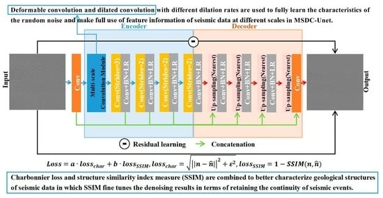
2.1. Network Architecture

The purpose of seismic data denoising is to attenuate the noise from the noisy data and recover an effective signal as much as possible. The mathematical model of denoising can be expressed as:
y = x + n ,
where y represents the noisy data contaminated by random noise, x is the clean data, n is the random noise.
The foundation of our method is the U-Net architecture. U-Net is a U-shaped convolution neural network structure based on Fully Convolutional Networks (FCNs), which is used to overcome the problems of FCNs. For example, a FCN cannot contact the context and location information, which is not suitable for complex tasks. The structure of U-Net makes it extract multi-level and multi-scale features, and the features extracted in the down-sampling process can be transferred to the up-sampling process through skip connection.
In order to enable U-Net to be competent for the task of seismic data denoising, we make some improvements to U-Net and propose a MSDC-Unet. As shown in Figure 1, we add a multi-scale convolution module to the network framework of the MSDC-Unet. The multi-scale convolution module is placed at the beginning of the network structure to maximize the advantages of multi-level and multi-scale feature extraction. The multi-scale convolution module mainly contains dilated convolution layers, feature fusion and deformable convolution, as illustrated in Figure 2a. The expansion of the receptive field of the network is realized by connecting the dilated convolution layers with different dilation rates in parallel. The parallel dilated convolution module can learn feature information of seismic data at different scales, which effectively improves the denoising efficiency. The deformable convolution can effectively change the range of the receptive field depending on the shape of the signal, which helps the network to fully learn the characteristics of the random noise. In the down-sampling process of U-Net, the computation is reduced and the receptive field is increased by dimension reduction operation. Furthermore, we use a convolution layer with two strides instead of the pooling layer to implement the process of down-sampling, which is able to avoid the information loss caused by the pooling layer. Additionally, skip connection is used between up-sampling and down-sampling to fuse features. In the following subsection, we will introduce the specific structure of multi-scale convolution module in detail.
In addition, we use four down-sampling layers and four up-sampling layers in the network. The convolution kernel of each convolution layer is set to 3 × 3 . The extraction of features and number of channels are realized through convolution. The numbers of filters in the process of Encoder are 16, 32, 128 and 256, respectively. The process of Decoder is the opposite. Batch normalization and activation function are added after convolution layer. Here, we replace the ReLU function with a LeakyReLU function to avoid the gradient disappearing. The convolution layer uses zero padding to keep the size of the feature map unchanged.

2.2. Multi-Scale Convolution Module

The structure of the multi-scale convolution module is shown in Figure 2a. The number of input and output channels is 16, and the convolution kernel size is 3 × 3 . In the module, the preliminary feature extraction of the input data are implemented through a convolution layer, and can be expressed as:
y 16 × 240 × 240 = c o n v 3 × 3 ( i n p u t 1 × 240 × 240 ) .
As shown in Figure 2a, we use dilated convolution with different dilation rates in a parallel three-layer structure. The convolution kernel size of the dilated convolution is 3 × 3 . Due to the different dilation rates, the features of the data extracted by the dilated convolution are also different. The dilated convolution with a large dilation rate extracts global information and the dilated convolution with a small dilation rate extracts local information.
y 1 = c o n v 3 × 3 ( y 16 × 240 × 240 ) ,   d i l a t i o n r a t e = 1 ,
y 2 = c o n v 3 × 3 ( c o n v 1 × 1 ( y 16 × 240 × 240 ) ) ,   d i l a t i o n r a t e = 3 ,
y 3 = c o n v 3 × 3 ( c o n v 1 × 1 ( y 16 × 240 × 240 ) ) ,   d i l a t i o n r a t e = 5 ,
where i n p u t is the input seismic noisy data, and y 1 , y 2 , y 3 are the feature map extracted from these three channels. In the multi-scale convolution module, dilated convolution with different dilation rates is used to extract the features of the seismic data at different scales, which results in a more comprehensive seismic data feature extraction.
Then, the results of the convolution of the three branches are feature fused, and the number of channels is reduced by using a 1 × 1 convolution to reduce the amount of network calculations. After the convolution operation, the LeakyReLU function and batch normalization are used to increase non-linearity, prevent overfitting, and improve the training efficiency of the model. Additionally, we add the deformable convolution at the end of the module, which can adjust the shape of the convolution kernel according to the different shapes of the seismic signal to improve the accuracy of feature extraction.
y 4 = c o n v 3 × 3 ( c o n v 1 × 1 ( c o n c a t ( y 1 , y 2 , y 3 ) ) ) ,
y 5 = d e c o n v 3 × 3 ( y 4 ) ,
y 6 = L e a k y R e L U ( B N ( y 5 ) ) ,
where c o n c a t represents the fusion of features, d e c o n v is the deformable convolution layer, y 5 is the feature extraction through the deformable convolution, and y 6 is the output of the multi-scale convolution module.
As shown in Figure 2b, the position change of grid sampling points is realized by the spatial offset learned by deformable convolution. The deformation of the convolution kernel is actually an offset of the sampling position. By adding offsets to the sampling points of the standard convolution, the convolution kernel is deformed, so that the network can adapt to the size and shape of the seismic event. Compared with the fixed rectangle convolution kernel of standard convolution, the sampling points of deformable convolution are closer to the receptive field center, so more effective receptive fields can be obtained. Experiment results in Section 3 show that the combination of multi-scale information in this way can improve denoising performance.

2.3. Loss Function

The denoising process in MSDC-Unet can be expressed as:
x ^ = F ( y , Θ ) ,
where F is a mapping function between y and x ^ . x ^ is the clean data predicted by the model from the input noisy data y. Θ is the hyperparameters of the MSDC-Unet architecture.
As mentioned above, we use the multi-scale convolution module to fully extract the features of seismic data, and use the skip connection to ensure that extracted features are fully utilized. Moreover, motivated by DnCNN, we use residual learning to avoid gradient disappearance and gradient explosion. The loss function can be written as:
L = a · ( l o s s c h a r ) + b · ( l o s s SSIM ) ,
l o s s c h a r = | | n n ^ | | 2 + ϵ 2 ,
l o s s SSIM = 1 SSIM ( n , n ^ ) ,
where l o s s SSIM is loss function based on SSIM, l o s s c h a r is the Charbonnier loss [41], n is the input noise, and n ^ is the predicted noise. a and b are the weight parameters that adjust the relative importance of these two losses. ϵ is a constant that is suggested to be 10 5 . The SSIM is added in the loss function to fine tune the denoising performance in terms of enhancing the continuity of the geological structures. Finally, we use Adam algorithm to optimize the loss function [42].

2.4. Synthetic Dataset

Denoising methods based on deep learning need a large amount of data as the training dataset for feature learning to obtain good optimization results. Due to the high difficulty and cost of field seismic data acquisition, we use the numerical simulation method to construct the training dataset. We use three mathematical models to synthesize the seismic data, namely Vertical Seismic Profile (VSP) data, the reflection seismic data and the Marmousi2 data, respectively. The synthetic seismic data obtained by the models is clean, so we add white Gaussian noise with different levels (different SNR randomly selected in the range of 17 to 27 dB) to the synthetic clean data to obtain the noisy seismic data.
VSP acquisition technology can provide a direct relationship between underground structure and ground measurement parameters, which is widely used in the field of geophysical exploration [43]. We use the reflectivity method to synthesize VSP data in MATLAB, and the synthesized data contains up-going and down-going waves [44,45]. In the simulation of VSP data, the dominant frequency of seismic source varies from 10 Hz to 60 Hz. Finally, we obtain 38 synthetic clean seismic datasets, where each seismic dataset is composed of 240 traces and 2048 samples with a sampling interval of 1 ms.
The reflection seismic data is composed of different hyperbolic seismic events [24]. Each example of the reflection seismic data contains 401 traces and 601 time samples with a time sampling rate of 2 ms. The dominant frequency and apparent velocity are randomly chosen in the range of 10–40 Hz and 1500–2400 m/s, respectively.
In addition, we generate the zero-offset seismic profile based on the Marmousi2 velocity model [46], named the Marmousi2 dataset. We use the convolution model to generate 95 seismic datasets through convolution the reflectivity series with Ricker wavelet. Each dataset contains 1530 traces and 1100 time samples with the time sample rate of being 1 ms.
In order to increase the diversity of network training samples, we choose seismic data (Bpvelanal2004) from Dataset (website: https://wiki.seg.org/wiki/2004_BP_velocity_estim--ation_benchmark_model/ (accessed on 10 October 2022)).
Consequently, we generate 115 clean synthetic seismic datasets, from which we randomly select 15 as the test data. By adding white Gaussian noise with different intensities to the clean seismic data, the noisy data are generated. For large-scale seismic data, in order to increase the feature extraction ability, it is bound to increase the training parameters while it leads to a reduction in the training efficiency. In order to improve training efficiency and reduce training costs, the training dataset is cropped into many small-scale samples. We use the sliding window method to divide the input noisy data into sample patches with sizes of 240 × 240 . By preprocessing three different synthetic data, and arranging sliding windows from left to right, 3258 patches in size of 240 × 240 are generated from training samples and 354 patches with the same size are generated from test set. In order to test the generalization ability of the model, 3100 samples are randomly selected from 3258 samples as training sets, the model is iteratively trained, and 354 samples are used as verification sets to verify and evaluate the model. The ratio of each type of data in the training dataset and the test dataset is shown in Table 1.

2.5. Selection of Parameters and Quantitative Analysis of Denoising Performance

The Adam algorithm with β 1 = 0.9 is used to train our model. It takes about 6 h to train our model on a Nvidia GeForce GTX 2080 GPU. In addition, the number of training epochs is set to 300.
We use the signal-to-noise ratio (SNR), mean square error (MSE) and SSIM as quantitative metrics and seismic difference profiles as qualitative metric to evaluate the network denoising effect. The calculation formulas of SNR, MSE and SSIM are as follows:
SNR = 10 l g | | x | | 2 | | n ^ | | 2 .
MSE = 1 N i = 1 N ( x ^ i x i ) 2 .
SSIM = ( 2 μ x μ x ^ + c 1 ) ( 2 σ x σ x ^ + c 2 ) ( μ x 2 + μ x ^ 2 + c 1 ) ( σ x 2 + σ x ^ 2 + c 2 ) .
where x and x i denote the clean seismic data, x ^ i denotes the denoised seismic data, N is the number of seismic data sets, n ^ is the predicted noise, μ x and μ x ^ are the mean values of clean seismic data and denoised seismic data, σ x and σ x ^ are the standard deviations of clean seismic data and denoised seismic data, respectively. c 1 and c 2 are constants. The higher the SNR value, the closer the denoising data are to the clean data. On the contrary, the closer the MSE is to 0, the smaller the difference between the denoising and clean data is. SSIM is an index to evaluate the similarity between the denoised seismic data and the clean seismic data, and it is close to 1, indicating a higher similarity.

3. Results

In this section, we compare the proposed MSDC-Unet with a number of deep learning methods and traditional denoising algorithms, including DnCNN, U-Net, Damped Rank Reduction (DRR) [47] and f-x filtering [4]. To ensure the fairness of the experiment, we increase the corresponding number of layers in the network framework comparable to the MSDC-Unet and corresponding parameters are selected consistently. DnCNN takes about 4 h and the U-Net takes more than one hour during the training. Compared with DnCNN and U-Net, the training process of MSDC-Unet is more complicated, and requires more computational time because the deformable convolution needs to calculate the position offset of each sampling point. The addition of deformable convolution improves the perception ability of local details. Our MSDC-Unet achieves the highest average SNR and SSIM, as well as lower MSE in the denoising results of synthetic data. Moreover, MSDC-Unet outperforms the deep learning denoising methods from the visualized results.

3.1. Synthetic Examples

Figure 3, Figure 4 and Figure 5 and Table 2 compare the denoising results of several existing methods with those of the proposed method in terms of denoising performance of synthetic seismic data.
There are 15 seismic data points in the test set, which are composed equally of three types of synthetic seismic data. Then, we obtain the average SNR by averaging the SNR over the five data of each type. Table 2 lists the average SNR, SSIM and MSE of denoising results with different methods. As shown in Table 2, the average SNR and SSIM improvement of other methods are smaller than MSDC-Unet, which means our proposed method is better than other methods in quantitative metrics. The smaller the MSE value, the better the denoising effect, and the MSE of our model on three types of seismic data is the smallest. Then, we compare the denoising effect of these methods in different types of seismic data through visualization.
The denoising results of VSP data are provided in Figure 3, which shows a visual comparison on the VSP data from the test dataset for the methods of DnCNN, U-Net, DRR and f-x filtering. Figure 3a–c are clean data, noisy data and noise data. Figure 3d,f,h shows the denoised results using f-x filtering, DRR and DnCNN, respectively. It can clearly be seen that a large amount of random noise still remains in those denoising data. Figure 3j,l shows the denoising results using U-Net and our proposed network, which are entirely cleaner than other methods. Figure 3e,g,i,k,m shows the removed noise corresponding to Figure 3d,f,h,j,l, and the signal loss is intuitive, compared with Figure 3c. Figure 3e shows strong signal leakage in the denoising results with f-x filtering. Figure 3g indicates that there is distinct signal damage in the coupling section of down-going waves and up-going waves in the method of DRR. Figure 3i shows that in the denoising results of DnCNN some effective signals are removed while a certain amount of noise is still retained in the denoising data of Figure 3h. Figure 3k,m illustrate that the U-Net and MSDC-Unet methods preserve the signals very well, which contain few down-going waves in the denoising results of U-Net and extremely few up-going waves in the denoising results of MSDC-Unet. It can be seen from the removed noise that there is some signal damage to the down-going wave in the denoising results of these methods, while obvious signal leakage also exists in up-going wave for other methods. The up-going wave with our method basically does not lose information. The SNR of noisy VSP seismic data are 9.31 dB. The SNR of the denoising data obtained by f-x filtering, DRR, DnCNN, U-Net, and MSDC-Unet are 14.26, 15.69, 23.77, 24.54, 25.63 dB, respectively. The MSDC-Unet has higher SSIM and lower MSE than other methods.
The clean data, noisy data and noise data for the second test data are shown in Figure 4a–c. The reflection seismic data consists of several hyperbolic seismic events, and the seismic signal structure is relatively simple [24]. Therefore, all of the denoising algorithms can recover the seismic signals to some extent. In Figure 4, we can clearly see that the denoising data obtained by our method (seen in Figure 4l,m) is the most similar to clean data and the noise removal is the most thorough. We can see that the signal leakage in Figure 4i,m is relatively small, but there is still a lot of residual noise in the denoising data as shown in Figure 4h for the method of DnCNN. It can be seen from Figure 4 that the denoising data with MSDC-Unet is cleaner and brighter than other methods, while there is almost no signal leakage in the removed noise. According to the evaluation index in Table 2, the improvements in SNR, SSIM and MSE of denoising data obtained by MSDC-Unet is the highest compared with other methods, in which the SNR and SSIM increase from 5.16 dB to 24.88 dB, from 0.849 to 0.997, and the MSE decreases from 0.01 to 9.99 × 10 5 , respectively, indicating that our method has the best denoising performance.
Figure 5a–c shows the clean data, noisy data and noise data from the Marmousi2 model. Figure 5d,f,h,j,l shows the denoising data using f-x filtering, DRR, DnCNN, U-Net, and MSDC-Unet, respectively. The steep interfaces part of the denoising results is zoomed to better show the denoising effect, as shown on the left side of Figure 5d,f,h,j,l. One can see that the denoising data through MSDC-Unet is much clearer than other methods, and many weak seismic signals in the enlarged parts are well restored. Figure 5d,h,j shows the seismic signal reconstructed by f-x filtering, DnCNN and U-Net is blurry and discontinuous, indicating that there is still a large amount of noise in the denoising data while the signal damage is relatively serious. Figure 5f,g illustrates that DRR strongly damages the seismic signal at the position of strong impedance contrasts and steep interfaces. The difference profiles in Figure 5e,i,k also confirm the disadvantage of these methods. From Figure 5e,i,k, it is clear that some geophysical structures in details are lost in the removed noise, which results in a decline in data quality. The seismic signals in Marmousi2 synthetic data are more complex and a large number of weak signals exist in these data, which requires higher performance of the denoising network framework. From Figure 5l,m, it can be seen that our method retains the most signal details compared with other methods and the denoising data are much cleaner and more continuous in geological structures, which corresponds to the improved SNR and SSIM in Table 2.
To further verify the denoising performance of the proposed method on seismic data with low SNR, Marmousi2 data with complex geological structures and amounts of weak signals are selected for testing. Figure 6a,b are clean data and noisy data, respectively. Figure 6c is noise data added in the Figure 6b. It can be found that, compared with Figure 5b, the noise level in Marmousi2 data increases and the initial SNR changes from −0.94 dB to −14.75 dB, making some weak signals hidden in the noise. Compared with other methods, the denoising results of DRR and MSDC-Unet are relatively clean and have less signal loss in the removed noise. It can be seen that there is residual noise in the denoising result through DRR, where the area indicated by the red arrows in Figure 6f, while the corresponding part of the noise in the result of MSDC-Unet is removed, as shown in Figure 6l. Figure 6g,m indicates that both DRR and MSDC-Unet damage the signal at the steep interfaces. From Figure 6d,e, it can be seen that f-x filtering cannot handle the mixing of signal and noise in the frequency domain. In the case of low SNR and hidden signals, the signal loss of DnCNN and U-Net is serious and they cannot recover weak signals well. In contrast, MSDC-Unet can recover weak signals while removing noise, which has better denoising performance.
From the perspective of the visual effect as shown in Figure 3, Figure 4, Figure 5 and Figure 6, MSDC-Unet has better effect on random noise denoising compared with other algorithms in the synthetic data.

3.2. Field Examples

To further verify the practicality of the proposed MSDC-Unet method, we apply it to three field seismic datasets to demonstrate its denoising performance. The denoising results of the MSDC-Unet method are also compared with those of other denoising methods.
To evaluate the denoising performance of our proposed network, Figure 7, Figure 8 and Figure 9 show the denoising results of three field seismic data. Figure 7a shows the first raw field seismic data. The corresponding denoising results are shown in Figure 7b,d,f,h,j, respectively. Figure 7c,e,g,i,k are residuals after noise suppression. From Figure 7a, we can find that the noise in the field seismic data are relatively strong, and there are many weak signals masked by noise. Although DRR can remove a lot of noise, the signal recover in part of region marked with the red box is not as good as MSDC-Unet. Figure 7b,c shows that, in the denoising results of f-x filtering, a lot of noise is removed, but visible effective signals are lost. It can be seen from Figure 7f that the DnCNN is also good at noise suppression, but the obvious block blur exists in the denoising data and the signal loss remains in difference profile of Figure 7g. Compared with the denoising results of Figure 7h,j, we can find that the MSDC-Unet can remove more noise than U-Net, and the signal leakage in Figure 7k is relatively small. Among the residual results, the signal loss in Figure 7k is the least. The denoising results demonstrate the MSDC-Unet has the ability of signal recovery and noise attenuation for field seismic data.
Figure 8a shows the second field seismic data, a type of distributed acoustic-sensing vertical seismic profile (DAS-VSP) with different types of noise such as random noise, optical cable vibration noise and instrument vibration noise. From Figure 8b–e, we can clearly see that f-x filtering and DRR do not thoroughly suppress the noise. The complex noise in Figure 8a is relatively strong, so it is difficult for traditional denoising methods to suppress the noise and recover weak signals. It can be seen from Figure 8f–i that DnCNN and U-Net methods perform better than the above two traditional denoising methods in noise attenuation. But Figure 8g,i show that the visible signals marked with red boxes are lost when recovering the data. In Figure 8j, MSDC-Unet method has relatively complete noise attenuation. Compared to the denoising results of DnCNN and U-Net, MSDC-Unet is better in terms of less signal leakage and relatively thorough noise suppression.
In Figure 9, we can clearly see that various types of noise exist in the DAS-VSP field seismic data, in addition to random noise, and the weak signals are strongly submerged in the complex noise. It can be observed that there is remaining noise in the denoised data, and the removed noise contains various degrees of signal loss in the other four methods. Comparing the part of the pure noise data marked with red boxes in Figure 9, the background in Figure 9j is cleaner than that of other methods. As shown in Figure 9j,k, the denoising results illustrate that MSDC-Unet can remove random noise and other types of noise to some extent.
Extensive experiments show that our MSDC-Unet is more efficient and has better performance than existing representative deep leaning and classical denoising methods. The noise suppression by DRR is completely in several field seismic data, but there is some signal leakage in the denoising results of DRR. The signal damage in the denoising data of f-x filtering and DnCNN is serious. The performance of U-Net is poor in some field seismic data, especially in the test of the third field seismic data, where there is a large amount of residual noise in the denoising results of U-Net. Visualization results show that MSDC-Unet can achieve a good balance between removing noise and recovering details of seismic signal.

4. Discussion

4.1. Parameters Selection in Multi-Scale Convolution Module

The purpose of seismic data denoising is to remove noise and recover effective signals as much as possible, according to the characteristics of random noise in seismic data [48]. Therefore, we propose MSDC-Unet model to fully extract noise features by using residual learning and a multi-scale convolution module. The multi-scale convolution module can extract features from different scales and improve the performance of feature extraction and denoising. Therefore, the parameter selection of the multi-scale convolution module is very important. In this work, we mainly use SNR to evaluate the denoising performance of seismic data. In order to obtain the best denoising performance, we tune the parameters of the multi-scale convolution module according to the SNR. The selection and results of the module parameters are shown in Table 3. First, we change the number of layers of the dilated convolution at each branch in Figure 2a. Second, we adjust the dilation rate of the dilated convolution in the module.
After repeated testings of the model performance using the parameters listed in Table 3, the optimal recommended parameters are shown in bold font (the second row). In Table 3, SNR represents the average SNR of the test set.
Through the analysis of Table 3, it can be found that the size of the receptive field has a significant impact on the feature extraction. When the receptive field is small, the extracted features are relatively local. Correspondingly, when the receptive field becomes large, the extracted features are more comprehensive. As can be seen from Table 3, it is clear that SNR is largest when the number of convolution layers used by the multi-scale convolution module are 1, 2, 2, the size of convolution kernel is 3 × 3 , and the dilation rate is 1, 3, 5. In this case, the corresponding receptive field size is 3, 7, 11. The results show that the use of larger receptive field size can improve the evaluation index, compared with the case of parameters in the second row and the last row, where the size of corresponding receptive fields is 3, 7, 11 and 1, 5, 9, respectively. Compared with the parameters in the second, third, and fourth rows, although the receptive field for the case of the second row is smaller than that of the third and fourth rows, it enables us to achieve less occupied resources and improve denoising precision compared to the choice of the other two parameters. This is because of the grid effect of dilated convolution, and continuous use of dilated convolution, may reduce feature extraction performance.

4.2. Loss Function Parameters Selection

The loss function measures the difference between the ground-truth and the predicted data. Different loss functions have different advantages and disadvantages. For practical problems, the corresponding loss function should be selected based on the real situation. As a common loss function for denoising problems, MSE has the advantage of fast convergence, but it is easily affected by outliers. Therefore, we choose Charbonnier loss as part of the loss function of the proposed method, which has better denoising performance and can better handle outliers. In this paper, due to the complex geological structures of seismic data, we add SSIM into the loss function to enable the seismic events continuous in the denoising data. SSIM can measure the structural similarity between two data, which makes the predicted data have higher structural continuity. In order to obtain the best denoising effect, we need to obtain the optimal weight through several experiments. We train the MSDC-Unet model through the weighted loss function with different weights, and test the trained model on the synthetic data. The test results are shown in Table 4.
When the constant ϵ is 10 5 , the denoising effect of the model is better. Then, we fix the constant ϵ and adjust the weights a and b. The results show that the best denoising performance is achieved when a = 0.001 and b = 0.999 in these experiments. The loss curve is shown in Figure 10. From Table 4, we can see that good denoising effect can be achieved using Charbonnier loss alone. However, the decline of loss curve is smoother and the values of MSE and SNR are more reasonable when combing the Charbonnier loss and SSIM. If the SSIM loss is added to the loss function for fine tuning, the structure of the denoising data can become more continuous. The results show that we can give full play to the advantages of each loss function by reasonable combination of different loss functions, so that they can better measure the similarity between the predicted data and the ground-truth and achieve satisfying denoising effect.

4.3. Strategy of Modifying the Network Structure

In this section, we perform ablation studies to demonstrate the role of the main components in the MSDC-Unet. Table 5 shows the SNR of denoising results on the synthetic dataset with different modules, where the first column shows the main components in the network, i.e., MFE, CS, DC. When MFE is selected, it means that the multi-scale convolution module, with the exclusion of deformable convolution, is used to replace standard convolution layer, whose position is shown in Figure 1. CS means that convolution layers with increased stride are used to replace max-pooling to implement down-sampling. DC indicates that the deformable convolution is added at the last layer of the MFE. The last column of Table 5 is our proposed MSDC-Unet. Table 5 indicates that the SNR for MSDC-Unet containing MFE, CS and DC modules is highest in the experimental results. In the MSDC-Unet, the MFE can change the receptive field to obtain contextual information from different scales and positions in the data. The DC can learn different noise features by changing the sampling locations. The CS can reduce unnecessary information loss in the down-sampling process. The deeper the network layer, the more abstract the information extracted. MFE and DC modules placed at the second layer of the network is conducive to the extraction of complete spatial information, which is transmitted to the deep network through the symmetric structure of U-Net to achieve the fusion of low-level features and high-level features. In order to enhance the roles of each modules of MFE, CS and DC, Figure 11 compares the feature maps of MSDC-Unet with those of U-Net. As shown in Figure 11, feature maps in the modules of MFE and DC are really different, suggesting that model with MFE and DC can extract more comprehensive features. The feature maps learned by U-Net (Figure 11d) are relatively similar to the input features, indicating that the effective information has not been learned much. In contrast, the features learned by different channels after deformable convolution (Figure 11b) are relatively different, which is beneficial for the subsequent noise suppression.
Although the computing cost and training time of the network increase slightly, the denoising effect of the model with the deformable convolution is obviously improved, and the increase in training time is acceptable. From Table 5 and Figure 12, it can be seen that each module such as MFE, CS and DC in the MSDC-Unet plays an important role and contributes to improve the denoising performance of the network. Moreover, we use the denoising results in Figure 11 as qualitative indicators to illustrate the denoising effects of different modules. The denoising results are consistent with the improvement in SNR. In Figure 11, we take the Marmousi2 synthetic experiment as an example to show the denoising effect of different modules. Figure 11a,b are clean data and noisy data. Figure 11c,e,g,i show denoising results using U-Net, U-Net with CS, U-Net with CS and MFE, respectively. The removed noise corresponding to them are shown in Figure 11d,f,h,j. It is clear that with the increase in modules in the network, signal leakage decreases. In Figure 11c,d, only strong signals are recovered and most weak signals are lost. In Figure 11f,h, there is some obvious signal leakage, but the signal loss is reduced in Figure 11h, indicating that the feature extraction ability of MFE effectively improves the model performance. The denoising results of MSDC-Unet are shown in Figure 11i,j, the signal leakge is the least in Figure 11j compared with Figure 11d,f,h. Therefore, it is reasonable to apply the multi-scale convolution module to the MSDC-Unet model.

4.4. Future Works

Although MSDC-Unet achieves a good denoising effect in synthetic seismic data, it still needs to be improved in field seismic data. First, the training dataset only contains random noise and four types of synthetic data, which is different from complex field seismic data with various types of noise. Second, the addition of multi-scale convolution module inevitably increases the training time. How to strengthen the generalization of the denoising model and decrease the training time also requires further research.

5. Conclusions

An effective denoising method is crucial for each step of the seismic data processing. In this paper, we propose a MSDC-Unet model with multi-scale convolution module to suppress random noise of seismic data. MSDC-Unet makes fully use of the extracted features of seismic data by adding modules of MFE, CS and DC. We introduce the dilated convolution with different dilation rates to extract both local and global information of the data. We use convolutional layer with two strides instead of the pooling layer to implement the process of down-sampling, which avoids the information loss caused by the pooling layer. The deformable convolution is utilized to adjust the shape of the convolution kernel according to the shapes of the input data to improve the accuracy of feature extraction. Moreover, because of residual learning, the training performance is improved and the problem of the gradient disappearance is avoided. In addition, we use ablation experiments to illustrate the necessary of MFE, CS and DC. For the model loss function, we combine Charbonnier loss and SSIM to effectively preserve the details of seismic data in which SSIM fine tunes the denoising results in terms of retaining the continuity of seismic events.
The experiments demonstrate that the MSDC-Unet has good performance in synthetic data and field data from the quantitative index and visualization effect. Compared with other methods such as f-x filtering, DRR, DnCNN and U-Net, the MSDC-Unet model can better suppress random noise and recover effective signal. However, the MSDC-Unet model still has some limitations to be solved, such as training efficiency and generalization to field seismic data. The above problems will be further improved in future work.

Author Contributions

All the authors made significant contributions to this work. Y.Z. and T.B. designed the framework of the network and performed the experiments; H.Z. and Y.Z. prepared the training dataset; H.Z., Y.Z., T.B. and Y.C. analyzed the results; Y.Z. and H.Z. wrote original draft of the paper; H.Z. and T.B. revised the paper; H.Z. acquired the funding support; Y.C. provided the field data; H.Z. is a supervision. All authors have read and agreed to the published version of the manuscript.

Funding

This research was funded by the National Key R&D Program of China under grant number 2021YFA0716901, the National Natural Science Foundation of China under grant number 41974132, the Fundamental Research Funds for the Central Universities under grant number xzy012023050 and BGP Scientific Research Project under grant number 03-03-06-2022.

Data Availability Statement

Part of synthetic seismic data and field data come from SEG open data (website: https://wiki.seg.org/wiki/Open_data/ (accessed on 11 October 2022)).

Acknowledgments

The authors would like to thank SEG and Gary S. Martin et al. for the open model: Marmousi2 and the open data. We would also like to thank the open source code of DRR (https://github.com/chenyk1990/MATdrr/ (accessed on 10 August 2022)) and deformable convolution (https://github.com/kastnerkyle/deform-conv/tree/master/deform_conv/ (accessed on 2 August 2022)) as well as SeismicLab package (https://github.com/msacchi/SeismicLab/ (accessed on 10 October 2022)).

Conflicts of Interest

The authors declare no conflict of interest.

References

  1. Chen, G.; Yang, W.; Liu, Y.; Wang, H.; Huang, X. Salt Structure Elastic Full Waveform Inversion Based on the Multiscale Signed Envelope. IEEE Trans. Geosci. Remote Sens. 2022, 60, 1–12. [Google Scholar] [CrossRef]
  2. Chen, G.; Yang, W.; Wang, H.; Zhou, H.; Huang, X. Elastic Full Waveform Inversion Based on Full-Band Seismic Data Reconstructed by Dual Deconvolution. IEEE Geosci. Remote Sens. Lett. 2022, 19, 1–5. [Google Scholar] [CrossRef]
  3. Yang, L.; Fomel, S.; Wang, S.; Chen, X.; Chen, W.; Saad, O.M.; Chen, Y. Denoising of distributed acoustic sensing data using supervised deep learning. Geophysics 2023, 88, WA91–WA104. [Google Scholar] [CrossRef]
  4. Abma, R.; Claerbout, J. Lateral prediction for noise attenuation by t-x and f-x techniques. Geophysics 1995, 60, 1887–1896. [Google Scholar] [CrossRef]
  5. Chen, T.; Ma, K.K.; Chen, L.H. Tri-state median filter for image denoising. IEEE Trans. Image Process. 1999, 8, 1834–1838. [Google Scholar] [CrossRef]
  6. Andrews, H.; Patterson, C. Singular value decompositions and digital image processing. IEEE Trans. Acoust. Speech Signal Process. 1976, 24, 26–53. [Google Scholar] [CrossRef]
  7. Bi, W.; Zhao, Y.; An, C.; Hu, S. Clutter Elimination and Random-Noise Denoising of GPR Signals Using an SVD Method Based on the Hankel Matrix in the Local Frequency Domain. Sensors 2018, 18, 3422. [Google Scholar] [CrossRef]
  8. Gilles, J. Empirical Wavelet Transform. IEEE Trans. Signal Process. 2013, 61, 3999–4010. [Google Scholar] [CrossRef]
  9. He, W.; Zhang, H.; Zhang, L.; Shen, H. Hyperspectral Image Denoising via Noise-Adjusted Iterative Low-Rank Matrix Approximation. IEEE J. Sel. Top. Appl. Earth Obs. Remote Sens. 2015, 8, 3050–3061. [Google Scholar] [CrossRef]
  10. Huang, W.; Wang, R.; Chen, Y.; Li, H.; Gan, S. Damped multichannel singular spectrum analysis for 3D random noise attenuation. Geophysics 2016, 81, V261–V270. [Google Scholar] [CrossRef]
  11. Zhuang, L.; Bioucas-Dias, J.M. Fast Hyperspectral Image Denoising and Inpainting Based on Low-Rank and Sparse Representations. IEEE J. Sel. Top. Appl. Earth Obs. Remote Sens. 2018, 11, 730–742. [Google Scholar] [CrossRef]
  12. Feng, J.; Li, X.; Liu, X.; Chen, C. Multigranularity Feature Fusion Convolutional Neural Network for Seismic Data Denoising. IEEE Trans. Geosci. Remote Sens. 2022, 60, 1–11. [Google Scholar] [CrossRef]
  13. Li, P.; Ren, P.; Zhang, X.; Wang, Q.; Zhu, X.; Wang, L. Region-Wise Deep Feature Representation for Remote Sensing Images. Remote Sens. 2018, 10, 871. [Google Scholar] [CrossRef]
  14. He, C.; Shi, Z.; Qu, T.; Wang, D.; Liao, M. Lifting Scheme-Based Deep Neural Network for Remote Sensing Scene Classification. Remote Sens. 2019, 11, 2648. [Google Scholar] [CrossRef]
  15. Tao, Y.; Muller, J.P. Super-Resolution Restoration of MISR Images Using the UCL MAGiGAN System. Remote Sens. 2019, 11, 52. [Google Scholar] [CrossRef]
  16. Zhang, X.; Liu, G.; Zhang, C.; Atkinson, P.M.; Tan, X.; Jian, X.; Zhou, X.; Li, Y. Two-Phase Object-Based Deep Learning for Multi-Temporal SAR Image Change Detection. Remote Sens. 2020, 12, 548. [Google Scholar] [CrossRef]
  17. Pei, J.; Huo, W.; Wang, C.; Huang, Y.; Zhang, Y.; Wu, J.; Yang, J. Multiview Deep Feature Learning Network for SAR Automatic Target Recognition. Remote Sens. 2021, 13, 1455. [Google Scholar] [CrossRef]
  18. Yu, S.; Ma, J. Deep Learning for Geophysics: Current and Future Trends. Rev. Geophys. 2021, 59, e2021RG000742. [Google Scholar] [CrossRef]
  19. Wang, B.; Zhang, N.; Lu, W.; Wang, J. Deep-learning-based seismic data interpolation: A preliminary result. Geophysics 2019, 84, V11–V20. [Google Scholar] [CrossRef]
  20. Liu, D.; Wang, W.; Wang, X.; Wang, C.; Pei, J.; Chen, W. Poststack Seismic Data Denoising Based on 3-D Convolutional Neural Network. IEEE Trans. Geosci. Remote Sens. 2020, 58, 1598–1629. [Google Scholar] [CrossRef]
  21. Sang, W.; Yuan, S.; Yong, X.; Jiao, X.; Wang, S. DCNNs-Based Denoising with a Novel Data Generation for Multidimensional Geological Structures Learning. IEEE Geosci. Remote Sens. Lett. 2021, 18, 1861–1865. [Google Scholar] [CrossRef]
  22. Wu, B.; Meng, D.; Zhao, H. Semi-Supervised Learning for Seismic Impedance Inversion Using Generative Adversarial Networks. Remote Sens. 2021, 13, 909. [Google Scholar] [CrossRef]
  23. Yu, J.; Wu, B. Attention and Hybrid Loss Guided Deep Learning for Consecutively Missing Seismic Data Reconstruction. IEEE Trans. Geosci. Remote Sens. 2022, 60, 1–8. [Google Scholar] [CrossRef]
  24. Zhao, H.; Bai, T.; Wang, Z. A Natural Images Pre-Trained Deep Learning Method for Seismic Random Noise Attenuation. Remote Sens. 2022, 14, 263. [Google Scholar] [CrossRef]
  25. Zhang, K.; Zuo, W.; Chen, Y.; Meng, D.; Zhang, L. Beyond a Gaussian Denoiser: Residual Learning of Deep CNN for Image Denoising. IEEE Trans. Image Process. 2017, 26, 3142–3155. [Google Scholar] [CrossRef] [PubMed]
  26. Ronneberger, O.; Fischer, P.; Brox, T. U-Net: Convolutional Networks for Biomedical Image Segmentation. In Proceedings of the Medical Image Computing and Computer-Assisted Intervention—MICCAI 2015: 18th International Conference, Munich, Germany, 5–9 October 2015; Navab, N., Hornegger, J., Wells, W.M., Frangi, A.F., Eds.; Springer: Cham, Switzerland, 2015; pp. 234–241. [Google Scholar]
  27. Yang, X.; Li, S.; Chen, Z.; Chanussot, J.; Jia, X.; Zhang, B.; Li, B.; Chen, P. An attention-fused network for semantic segmentation of very-high-resolution remote sensing imagery. ISPRS J. Photogramm. Remote Sens. 2021, 177, 238–262. [Google Scholar] [CrossRef]
  28. Gui, Y.; Li, W.; Xia, X.G.; Tao, R.; Yue, A. Infrared Attention Network for Woodland Segmentation Using Multispectral Satellite Images. IEEE Trans. Geosci. Remote Sens. 2022, 60, 1–14. [Google Scholar] [CrossRef]
  29. Zhu, W.; Mousavi, S.M.; Beroza, G.C. Seismic Signal Denoising and Decomposition Using Deep Neural Networks. IEEE Trans. Geosci. Remote Sens. 2019, 57, 9476–9488. [Google Scholar] [CrossRef]
  30. Kaur, H.; Fomel, S.; Pham, N. Seismic ground-roll noise attenuation using deep learning. Geophys. Prospect. 2020, 68, 2064–2077. [Google Scholar] [CrossRef]
  31. Dong, X.; Wang, H.; Zhong, T.; Li, Y. PDN: An effective denoising network for land prestack seismic data. J. Appl. Geophys. 2022, 199, 104558. [Google Scholar] [CrossRef]
  32. Li, Y.; Zhang, M.; Zhao, Y.; Wu, N. Distributed Acoustic Sensing Vertical Seismic Profile Data Denoising Based on Multistage Denoising Network. IEEE Trans. Geosci. Remote Sens. 2022, 60, 1–17. [Google Scholar] [CrossRef]
  33. Liu, D.; Deng, Z.; Wang, C.; Wang, X.; Chen, W. An Unsupervised Deep Learning Method for Denoising Prestack Random Noise. IEEE Geosci. Remote Sens. Lett. 2022, 19, 1–5. [Google Scholar] [CrossRef]
  34. Zhong, T.; Cheng, M.; Lu, S.; Dong, X.; Li, Y. RCEN: A Deep-Learning-Based Background Noise Suppression Method for DAS-VSP Records. IEEE Geosci. Remote Sens. Lett. 2022, 19, 1–5. [Google Scholar] [CrossRef]
  35. Saad, O.M.; Chen, Y. A fully unsupervised and highly generalized deep learning approach for random noise suppression. Geophys. Prospect. 2021, 69, 709–726. [Google Scholar] [CrossRef]
  36. Dong, X.; Li, Y.; Zhong, T.; Wu, N.; Wang, H. Random and Coherent Noise Suppression in DAS-VSP Data by Using a Supervised Deep Learning Method. IEEE Geosci. Remote Sens. Lett. 2022, 19, 1–5. [Google Scholar] [CrossRef]
  37. Li, J.; Wu, X.; Hu, Z. Deep Learning for Simultaneous Seismic Image Super-Resolution and Denoising. IEEE Trans. Geosci. Remote Sens. 2022, 60, 1–11. [Google Scholar] [CrossRef]
  38. Gao, Z.; Zhang, S.; Cai, J.; Hong, L.; Zheng, J. Research on Deep Convolutional Neural Network Time-Frequency Domain Seismic Signal Denoising Combined With Residual Dense Blocks. Front. Earth Sci. 2021, 9, 681869. [Google Scholar] [CrossRef]
  39. Bai, T.; Zhao, H.; Wang, Z. A U-Net Based Deep Learning Approach for Seismic Random Noise Suppression. In Proceedings of the IGARSS 2022—2022 IEEE International Geoscience and Remote Sensing Symposium, Kuala Lumpur, Malaysia, 17–22 July 2022; pp. 6165–6168. [Google Scholar]
  40. Zhao, H.; Bai, T.; Chen, Y. Background Noise Suppression for DAS-VSP Records Using GC-AB-Unet. IEEE Geosci. Remote Sens. Lett. 2022, 19, 1–5. [Google Scholar] [CrossRef]
  41. Liang, J.; Cao, J.; Sun, G.; Zhang, K.; Van Gool, L.; Timofte, R. SwinIR: Image Restoration Using Swin Transformer. In Proceedings of the 2021 IEEE/CVF International Conference on Computer Vision Workshops (ICCVW), Montreal, BC, Canada, 11–17 October 2021; pp. 1833–1844. [Google Scholar]
  42. Kingma, D.P.; Ba, J. Adam: A Method for Stochastic Optimization. arXiv 2014, arXiv:1412.6980. [Google Scholar]
  43. Zhao, Q.; Miao, Z.; Xu, W.; Song, S. A multi-scale adaptive feature enhancement network for image denoising. In Proceedings of the Thirteenth International Conference on Signal Processing Systems (ICSPS 2021), Shanghai, China, 12–15 November 2021; Li, Q., Mao, K., Xie, Y., Eds.; International Society for Optics and Photonics (SPIE): Bellingham, WA, USA, 2022; Volume 12171, p. 1217117. [Google Scholar]
  44. Ganley, D.C. A method for calculating synthetic seismograms which include the effects of absorption and dispersion. Geophysics 1981, 46, 1100–1107. [Google Scholar] [CrossRef]
  45. Zhao, H.; Gao, J.; Peng, J. Extended reflectivity method for modelling the propagation of diffusive–Viscous wave in dip-layered media. Geophys. Prospect. 2017, 65, 246–258. [Google Scholar] [CrossRef]
  46. Martin, G.; Wiley, R.; Marfurt, K. Marmousi2: An elastic upgrade for Marmousi. Lead. Edge 2006, 25, 156–166. [Google Scholar] [CrossRef]
  47. Chen, Y.; Huang, W.; Zhang, D.; Chen, W. An open-source Matlab code package for improved rank-reduction 3D seismic data denoising and reconstruction. Comput. Geosci. 2016, 95, 59–66. [Google Scholar] [CrossRef]
  48. Guo, L.; Luo, R.; Li, X.; Zhou, Y.; Juanjuan, T.; Lei, C. Seismic Random Noise Removal Based on a Multiscale Convolution and Densely Connected Network for Noise Level Evaluation. IEEE Access 2022, 10, 13911–13925. [Google Scholar] [CrossRef]
Figure 1. The structure of MSDC-Unet. Encoder and Decoder are marked with green and blue boxes, respectively. The structure of multi-scale convolution module is shown in Figure 2a.
Remotesensing 15 04569 g001
Figure 2. (a) The structure of multi-scale convolution module, where d denotes dilation rate. (b) The offsets of deformable convolution.
Remotesensing 15 04569 g002
Figure 3. VSP synthetic data. (a) Clean data. (b) Noisy data. (c) Noise data. Denoised data using: (d) f-x filtering, (f) DRR, (h) DnCNN, (j) U-Net, (l) MSDC-Unet. Removed noise using: (e) f-x filtering, (g) DRR, (i) DnCNN, (k) U-Net, (m) MSDC-Unet. The locations of signal loss are marked with red arrows.
Remotesensing 15 04569 g003aRemotesensing 15 04569 g003b
Figure 4. Reflection synthetic data. (a) Clean data. (b) Noisy data. (c) Noise data. Denoised data using: (d) f-x filtering, (f) DRR, (h) DnCNN, (j) U-Net, (l) MSDC-Unet. Removed noise using: (e) f-x filtering, (g) DRR, (i) DnCNN, (k) U-Net, (m) MSDC-Unet. The locations of signal loss are marked with red arrows.
Remotesensing 15 04569 g004aRemotesensing 15 04569 g004b
Figure 5. Marmousi2 synthetic data. (a) Clean data. (b) Noisy data. (c) Noise data. Denoised data using: (d) f-x filtering, (f) DRR, (h) DnCNN, (j) U-Net, (l) MSDC-Unet. Removed noise using: (e) f-x filtering, (g) DRR, (i) DnCNN, (k) U-Net, (m) MSDC-Unet. The denoising results in the red boxes in (d,f,h,j,l) are zoomed to the left. The locations of signal loss are marked with red arrows. The steep interfaces part of the denoising results marked by red box is zoomed on the left sides (d,f,h,j,l) of the figure.
Remotesensing 15 04569 g005aRemotesensing 15 04569 g005b
Figure 6. Marmousi2 synthetic data with low SNR. (a) Clean data. (b) Noisy data. (c) Noise data added. Denoised data using: (d) f-x filtering, (f) DRR, (h) DnCNN, (j) U-Net, (l) MSDC-Unet. Removed noise using: (e) f-x filtering, (g) DRR, (i) DnCNN, (k) U-Net, (m) MSDC-Unet. The locations of signal loss are marked with red arrows.
Remotesensing 15 04569 g006aRemotesensing 15 04569 g006b
Figure 7. First field seismic data. (a) Raw field data. Denoised data using: (b) f-x filtering, (d) DRR, (f) DnCNN, (h) U-Net, (j) MSDC-Unet. Removed noise using: (c) f-x filtering, (e) DRR, (g) DnCNN, (i) U-Net, (k) MSDC-Unet. The locations of signal loss are marked with red boxes.
Remotesensing 15 04569 g007aRemotesensing 15 04569 g007b
Figure 8. Second field seismic data. (a) Raw field data. Denoised data using: (b) f-x filtering, (d) DRR, (f) DnCNN, (h) U-Net, (j) MSDC-Unet. Removed noise using: (c) f-x filtering, (e) DRR, (g) DnCNN, (i) U-Net, (k) MSDC-Unet. The locations of signal loss are marked with red boxes.
Remotesensing 15 04569 g008aRemotesensing 15 04569 g008b
Figure 9. Third field seismic data. (a) Raw field data. Denoised data using: (b) f-x filtering, (d) DRR, (f) DnCNN, (h) U-Net, (j) MSDC-Unet. Removed noise using: (c) f-x filtering, (e) DRR, (g) DnCNN, (i) U-Net, (k) MSDC-Unet. The locations of pure noise data are marked with red boxes.
Remotesensing 15 04569 g009aRemotesensing 15 04569 g009b
Figure 10. The loss curve of MSDC-Unet in 500 epochs.
Remotesensing 15 04569 g010
Figure 11. Denoising results of different modules in MSDC-Unet on Marmousi2 synthetic data. (a) Clean data. (b) Noisy data. Denoised data using: (c) U-Net, (e) U-Net with CS, (g) U-Net with CS and MFE, (i) U-Net with CS, MFE and DC (MSDC-Unet). Removed noise using: (d) U-Net, (f) U-Net with CS, (h) U-Net with CS and MFE, (j) U-Net with CS, MFE and DC (MSDC-Unet). The locations of signal loss are marked with red arrows.
Remotesensing 15 04569 g011aRemotesensing 15 04569 g011b
Figure 12. Visualization of the feature maps in MSDC-Unet and U-Net. The first row is feature maps of MFE, DC and CS modules. The second row shows the corresponding feature maps of U-Net. (a) The feature map of MSDC-Unet after MFE module. (b) The feature map of MSDC-Unet after DC module. (c) The feature map of MSDC-Unet after CS module. (d) The feature map of U-Net after convolution. (e) The feature map of U-Net after down-sampling by max-pooling.
Remotesensing 15 04569 g012
Table 1. Quantity of the train dataset and the test dataset allocations. The size of each patch is 240 × 240 .
DatasetsThe Training DatasetsThe Test Datasets
VSP data800139
Reflection seismic data80035
Marmousi2 data800180
Bpvelanal2004700-
Total3100354
Table 2. Denoising results of synthetic data.
DatasetVSP DataReflection Seismic DataMarmousi2 Data
Evaluation indexesSNR/dBMSESSIMSNR/dBMSESSIMSNR/dBMSESSIM
Initial value9.31 5.47 × 10 3 0.9385.160.010.849−0.92 7.75 × 10 3 0.629
f-x filtering14.26 1.78 × 10 3 0.9712.93 2.08 × 10 3 0.95413.24 2.65 × 10 4 0.949
DRR15.69 1.19 × 10 3 0.98516.24 6.66 × 10 4 0.98713.34 2.6 × 10 4 0.974
DnCNN23.77 2.31 × 10 4 0.99620.92 2.32 × 10 4 0.98914.25 2.11 × 10 4 0.949
U-Net24.54 1.92 × 10 4 0.98722 1.93 × 10 4 0.9314.82 1.86 × 10 4 0.941
MSDC-Unet 25 . 63 1 . 69 × 10 4 0 . 997 24 . 88 9 . 99 × 10 5 0 . 997 17 . 58 9 . 69 × 10 5 0 . 987
Bold text represents the denoising effect of MSDC-Unet.
Table 3. Quantitative comparison of different parameters for multi-scale convolution module.
Number of Convolution LayersDilation RateConvolution KernelSNR/dB
Branch1Branch2Branch3Branch1Branch2Branch3Branch1Branch2Branch3
1111353 × 33 × 33 × 315.23
1 2 2 1 3 5 3 × 3 1 × 1 , 3 × 3 1 × 1 , 3 × 3 16 . 44
2221353 × 33 × 33 × 314.82
3331353 × 33 × 33 × 313.74
1231221 × 11 × 1, 3 × 31 × 1, 3 × 315.13
Bold text represents the parameter selection for the best SNR.
Table 4. Quantitative comparison of different weights for loss function.
ab ϵ MSESNR/dB
-- 10 3 0.017517.52
-- 10 4 0.012516.81
-- 10 5 0.011318.12
0.90.1 10 5 0.008517.57
0.990.01 10 5 0.009817.67
0.9950.005 10 5 0.007917.62
0 . 999 0 . 001 10 5 0 . 0089 18 . 5
Bold text represents the parameter selection for the best SNR.
Table 5. Quantitative comparison of ablation experiments.
MFE
DC
CS
SNR/dB12.5114.9316.0817.58
Bold text represents the parameter selection for the best SNR.
Disclaimer/Publisher’s Note: The statements, opinions and data contained in all publications are solely those of the individual author(s) and contributor(s) and not of MDPI and/or the editor(s). MDPI and/or the editor(s) disclaim responsibility for any injury to people or property resulting from any ideas, methods, instructions or products referred to in the content.

