Article

Double Inversion Layers Affect Fog–Haze Events over Eastern China—Based on Unmanned Aerial Vehicles Observation

1
School of Atmospheric Sciences, Chengdu University of Information Technology, Chengdu 610225, China
2
Key Laboratory of Transportation Meteorology of China Meteorological Administration, Nanjing Joint Institute for Atmospheric Sciences, Nanjing 210041, China
3
Lianyungang Meteorological Bureau of Jiangsu Province, Lianyungang 222000, China
*
Author to whom correspondence should be addressed.
Remote Sens. 2023, 15(18), 4541; https://doi.org/10.3390/rs15184541
Submission received: 7 August 2023 / Revised: 6 September 2023 / Accepted: 13 September 2023 / Published: 15 September 2023

Abstract

:
The goal of this work is to analyze how double inversion layers affect fog–haze events and boundary layers over Eastern China based on unmanned aerial vehicle observations. During 10–12 December 2020, two successive fog–haze events occurred in Eastern China. Based on the unmanned aerial vehicle (UAV), wind, temperature, relative humidity (RH), and aerosol mass concentration were monitored simultaneously in Lianyungang, China. Several observations were found after analyzing the physical fields of these data. The results show that the concentrations of air pollutants during fog events were negatively correlated with horizontal visibilities. The mass concentrations of particulate matter increased rapidly (After 08:00 BJT 11) in the fog dissipation stages (PM2.5 and PM10 increased from 97 and 150 μg/m3 to 213 and 300 μg/m3, respectively). Double temperature inversion significantly affected fog events, where the enhancement of the lower-level temperature inversion (where the inversion layer top height was between 150 and 300 m) corresponded to the explosive growth of fog and the dissipation of the upper-level inversion layer. (The bottom height of the inversion layer was between 350 m and 600 m) This indicates the end of fog events. Fog layer thicknesses are negatively correlated with the concentrations of air pollutants in the near-surface layer. The thickening of the inversion layer near the surface corresponds to an increase (after 05:00 BJT 11 and 03:00 BJT 12) in fog layer height. The fog event is maintained when water vapor conditions are favorable enough or when there is a deep near-surface temperature inversion but the maintenance of the near-surface temperature inversion at an intensity of above 2 °C (100 m)−1 mainly contributes to the durations of these two fog events. Calculations through the trajectory model reveal that the air pollutant source varied during these two events, which was the main reason for the difference in air pollutant concentrations between the two events.

Graphical Abstract

1. Introduction

In recent years, the frequent occurrence of fog–haze weather has caused serious harm to traffic safety and human health [1,2,3], which has attracted close attention from society. With rapid socioeconomic development and urbanization, increasing pollutants have been emitted into the atmosphere through human activities and industrial production, causing serious air pollution. In addition, haze weather, which often induces obstruction to vision, has become a high incidence of disastrous weather phenomena in urban agglomerations in both central and eastern China [4,5].
Meteorological conditions greatly influence the formation and maintenance of haze weather, which also plays an important role in the transportation, diffusion, transformation, and removal of atmospheric pollutants [6,7,8,9]. In studies on meteorological conditions related to haze pollution, meteorological measurements and analysis, as well as field observations of atmospheric pollutants, are among the most common research methods [10,11,12]. Meteorological observation data can help clarify the spatiotemporal variation characteristics of both meteorological factors and mass concentrations of atmospheric pollutants during haze pollution. Previous studies have revealed that favorable circulation situations, atmospheric stability, and humidity conditions are vital to enhancing the long-term maintenance of haze weather [13,14]. The long-term existence of continental high and temperature inversion provides a common background for haze pollution in China [15,16].
Some scholars have proposed that the haze pollution degree is closely related to a variation in meteorological elements in the boundary layer [17,18]. Complicated interactions are found among the water vapor, dynamic, and thermal conditions in the boundary layer, where the configuration of meteorological conditions determines the evolution characteristics of haze processes [19,20]. The mass concentration of pollutants is not only related to the emissions level of local pollutants but is also affected by transport among different regions [21,22]. With the development of urbanization and industrialization, air pollution has become a notable problem in China and is mainly concentrated in three major regions: the North China Plain [23], the Yangtze River Delta [24,25], and the Pearl River Delta [26,27].
In recent years, unmanned aerial vehicles (UAVs) have been widely applied to meteorological observations in the boundary layer. Due to their advantages of hovering, quasi-vertical takeoff and landing capabilities, stable flight speed, and high-frequency observation ability, UAVs have become indispensable tools for vertical analysis in the atmospheric boundary layer [28,29]. Unlike the traditional sounding balloon and tethered balloon-sounding observations, UAVs are more stable in their vertical measurement, maintaining a constant low speed during the observation process so that measurements are not affected by lifting speed [30]. Compared with satellite remote sensing and radar observations, UAVs can provide high spatiotemporal resolution observations. Moreover, the contact detection mode of UAVs is less affected by external factors, which ensures measurement accuracy to a larger extent [31,32]. Therefore, the application of UAV-sounding data contributes to the in-depth study of the atmospheric boundary layer.
Donghai County is located in the west of Lianyungang City, Jiangsu Province, which is located in the Yangtze River Economic Belt. This region is located on the coast, is economically developed, and fog and haze weather-prone [33,34]. Hence, the study of boundary layer features during haze processes and its relationship with air pollution is of great significance to people’s livelihoods and economic development. Although there have been abundant achievements in studies of haze pollution, most of them have focused on boundary layer features during the life history of one single case, and research data are mostly from the observations of surface meteorological observing stations [35,36]. In this study, the boundary layer features and variation characteristics of air pollutants during two haze events on 10–12 December 2020 were investigated based on the combination of UAV-sounding observations and ground-based conventional observations.
The rest of this manuscript is organized as follows. The study area and observation sites are described in Section 2. Synoptic situations and boundary layer features are analyzed in Section 3. Finally, the discussions and main conclusions are given in Section 4 and Section 5.

2. Observation and Analysis

2.1. Observation Site

The study area was located in Donghai, Lianyungang City, Jiangsu Province, which is a region about 50 km west of the Yellow Sea with a flat topography. The observation site has the same geographic location as that of the National Meteorological Observing Station of Donghai (34.54°N, 118.71°E, with an altitude of 32.9 m). It is located in the northern part of Jiangsu Province, western Lianyungang City, 3 km away from the urban area of Donghai, and is surrounded by flat and open areas without obstructions. Its geographical location is illustrated in Figure 1. The observation experiment of haze events performed in Donghai helped to reveal the characteristics of the fog–haze boundary layer and the formation of the pollution process in northern Jiangsu. An observational experiment on haze processes in northern Jiangsu was conducted here in December 2020.

2.2. Observation Data of Ground Meteorological Elements and Air Pollutants

Conventional meteorological observation data with a temporal resolution of 1 min were provided by the Meteorological Bureau of Donghai, including the atmospheric horizontal visibility (VIS), temperature, relative humidity (RH), wind direction, and wind speed. Specifically, the elements of temperature, RH, wind direction, and wind speed were collected from the DZZ4-type automatic weather station produced by Jiangsu Radio Science Research Institute Ltd., Nanjing, China, while atmospheric horizontal visibility was measured by a CJY-1G forward scattering atmospheric horizontal visibility sensor produced by the CAMA (Luoyang, China) Environmental Measurement Co., Ltd.
Hourly averaged air pollutant data (PM2.5 and PM10 concentrations) were provided by the national environmental monitoring station in Donghai, which and collected through the BAM-1020 ambient particulate (PM10 and PM2.5) monitor.

2.3. UAV Platforms

Sounding data were obtained using a UAV-based integrated boundary layer meteorological sounding system, including temperature, RH, wind direction, and wind speed. The UAV had a measurement frequency of 1 s each time, a vertical lifting speed of 150–200 m (min)−1, and received measurements at a vertical spatial resolution of 2.5–3 m. Temperature and RH in the sensor design use the sounding observation system, and this sensor has high sensitivity and accuracy. The solid-state pressure sensor is used to achieve instantaneous wind speed and wind direction measurements. In order to avoid the influence of rotor turbulence, the sensor was set up 60 cm above the height of the UAV arm, using a three-pillar structure to ensure stable support and effectively avoid resonance. Table 1 indicates the sensor parameters of the UAV boundary layer meteorological integrated detection system [12]. In this research, UAV observation data were compared with other sounding data [12]. In terms of precision and accuracy, UAV observation data performed best. There were 21 UAV detection processes conducted during the observation period. The detection range of the UAV was performed from the land surface to the height of 800 m above the ground.

2.4. Background Data

In this study, the instrumental observation of atmospheric horizontal visibility was classified into five levels based on a meteorological standard. It was defined as a slight haze when 5 km ≤ VIS < 10 km, a mild haze when 3 km ≤ VIS < 5 km, a moderate haze when 2 km ≤ VIS < 3 km, a severe haze when 1 km ≤ VIS < 2 km, and fog when VIS < 1 km [37].
Based on the Global Land Data Assimilation System dataset at a spatial resolution of 1° × 1° (ftp://ftp.arl.noaa.gov/archives/gdas1/, accessed on 10 January 2020), the Hybrid Single Particle Lagrangian Integrated Trajectory Model version 5 (HYSPLIT5.0) developed by the National Oceanic and Atmospheric Administration was used to calculate the backward trajectory. HYSPLIT is a professional model for calculating and analyzing the transport and diffusion trajectories of atmospheric pollutants. This model is a hybrid calculation model of Euler and Lagrangian models. Advection and diffusion were treated using the Lagrangian method, while the concentration was calculated by the Euler method [38].

3. Results

3.1. Synoptic Situations

From 10 to 12 December 2020, a severe fog–haze process occurred in Eastern China, while atmospheric circulation strongly affected this process. From the surface’s synoptic situation (image omitted), central and eastern China was dominated by the uniform pressure south of Mongolian high-pressure on the night of 10 December. On 11 and 12 December, eastern China was located at the top of a low-pressure inverted trough and influenced by easterly winds. At this time, the synoptic situation for the haze process changed from a uniform-pressure type to a low-pressure inverted trough type.

3.2. Surface Meteorological Conditions and Air Pollution

From 17:00 BST (Beijing Standard Time, the same as below) on 10 December to 12:00 BST on 12 December 2020, the VIS at Donghai station of Lianyungang was less than 4000 m (Figure 2). The durations of VIS were less than 3000 m, 2000 m, and 1000 m and lasted nearly 42 h, 38 h, and 16 h, respectively. During this haze pollution process, there were two conversion processes of “moderate haze–heavy haze–fog–heavy haze–moderate haze”. On this basis, the total haze period was divided into five sub-categories, as shown in Table 2. On the morning of 11 December and the night of 11 December to the morning of 12 December, the two fog processes lasted 4.7 h and 10.7 h, the duration of VIS below 500 m were 2.2 h and 6.3 h, and the minimum VISs were 45 m and 42 m, respectively.
Figure 2 shows the hourly variations in surface VIS, temperature, RH, wind direction, wind speed, and atmospheric particulate concentration from 10–12 December 2020 in Donghai. The temperature and RH presented obvious diurnal variation characteristics but also showed opposite change trends.
In the fog event, the difference between the temperature and the dew point was small, while RH was large and close to saturation. After the fog event, the temperature was significantly higher than the dew point, and RH decreased rapidly. Similarly, RH and VIS also presented opposite change trends—VIS increased (decreased) during the daytime (nighttime) while RH decreased (increased). The northwesterly and southwesterly winds prevailed around the near surface, with the wind speed mostly below 4 m/s. These two fog events were mainly dominated by westerly winds with a wind speed generally below 3 m/s. In addition, the VIS and wind speed exhibited synchronous change trends; that is, VIS increased (decreased) when the wind speed increased (decreased).
Temperature and VIS trends were consistent in their variation trends, where VIS decreased (increased) as the temperature decreased (increased). Minimal temperature values were found in the two fog events, which were −1.3 °C and −2.8 °C, respectively. The occurrence time of minimum temperature lagged far behind that of the minimum VIS for both fog events. After reaching the minimum VIS during the two fog events, the temperature continued to decrease, and the lagged time was 80 min and 50 min, respectively. On the morning of the 11th, due to the short duration of the fog event, the increase in the pollutant concentration after 0800 BST could be related to the increase in vehicle traffic during the morning rush hour. The fog event on the 12th was stronger and lasted longer. At this time, the mass concentration of PM10 did not continue to increase compared with that on the 11th.
The concentration of PM can be related to RH [39,40]. As shown in Figure 2 and Figure 3, the increase in RH in a short time could increase the concentration of PM (which is related to the hygroscopic growth of particles), while the high humidity environment (RH > 90%) for a long time (>12 h) decreased the concentration of particulate matter (wet scavenging effect). Due to the small RH (concentrated below 80%) during the haze process, the concentration of PM was also large (PM2.5 is concentrated in 200~280 μg/m3; PM10 was concentrated in 250~330 μg/m3), also indicating that the concentration of PM increased in the early stages of a high-humidity environment.
During the five stages of the haze events from 10 to 12 December, the mass concentration of atmospheric particulate matter fluctuated greatly. The mass concentration of PM2.5 was above 75 μg/m3, while that of PM10 was above 150 μg/m3 [41]). In the two fog events, the mass concentrations of PM2.5 were in the ranges of 97–128 μg/m3 and 196–306 μg/m3, with the mean values between 108 μg/m3 and 266.1 μg/m3, respectively. While the mass concentrations of PM10 were within the 150–209 μg/m3 and 306–390 μg/m3 range, the average values were 168 μg/m3 and 341.4 μg/m3, respectively.
Particulate matter mass concentrations differed greatly during these two fog events. In the first event, the mass concentrations of PM2.5 and PM10 presented the same change trend. At the beginning of fog formation, the mass concentration of particulate matter decreased as VIS decreased, which dropped to the bottom value at 07:00 BST on 11 December, when the mass concentrations of PM2.5 and PM10 were 97 μg/m3 and 150 μg/m3 and atmospheric horizontal visibility was 72 m. Afterward, the mass concentration of particulate matter continued to increase as VIS increased.
During the dissipation stage, the mass concentration increased rapidly. After 07:00 BST on 11 December, the intensity of the fog began to weaken and entered the dissipation stage. At this time, the morning peak began. Due to an increase in human activities and automobile emissions, the concentration of particulate matter increased. After 08:00 BST, the fog dissipated faster, and the concentration of particulate matter increased rapidly. After the fog disappeared, the mass concentrations of PM2.5 and PM10 reached the peak values of 213 μg/m3 and 300 μg/m3, respectively. By using the observation and WRF–Chem simulation, Qian et al. [42] found that fog had removal effects on the particulate matter.
However, the variation in PM2.5 mass concentrations was significantly different from that of PM10 during the second event. Since the beginning at 23:48 BST on 11 December, VIS slowly decreased while the mass concentration of particulate matter increased slightly. At 03:00 BST on 12 December, VIS dropped from 481 m to 302 m at 03:50 BST on 12 December before increasing increased to 991 m again. The mass concentrations of PM2.5 and PM10 began to show opposite change trends. From 03:00 BST to 09:00 BST on 12 December, VIS decreased to 51 m in a fluctuating way, while PM2.5 mass concentration continued to drop to its lowest at 196 μg/m3. After 09:00 BST, the PM2.5 mass concentration increased to 260 μg/m3 as VIS gradually increased. From 09:00 BST to 10:00 BST on 12 December, the VIS changed more slowly compared to that from 10:00 BST to the dissipation stage.
The mass concentration of PM2.5 exhibited greater changes, which was consistent with that during the dissipation stage of the first event. From 03:00 BST to 06:00 BST, the mass concentration of PM10 decreased from 355 μg/m3 to 329 μg/m3, with VIS dropping to 251 m at this stage. From 06:00 BST to 08:00 BST, the mass concentration of PM10 increased to 390 μg/m3 as VIS further decreased with a minimum VIS of 42 m at 06:40 BST. The PM10 mass concentration started to decrease after the fog gradually reached the maturity stage. During the dissipation stage, the mass concentration of PM10 changed rather slowly compared to the rapid change in VIS. Wu et al. [36] and Sun et al. [35] studied the Chemical Characteristics of PM2.5 and PM10 in Haze−Fog episodes around and in Beijing, and they found that some small particles grew into larger particles during the fog episode.
In short, the second fog event lasted longer than the first event, with stronger intensity. From the perspective of surface meteorological elements, the lower temperature and smaller wind speed during the second fog event were more favorable to the formation and maintenance of fog. The variation characteristics of pollutant matter mass concentrations varied greatly in the two fog events, and PM concentrations in the second fog event were, on average, four times higher than that in the first one because of the Koehler and Kelvin effect; PM and aerosol might also trigger or intensify fog due to the hygroscopicity of particles, indicating that the pollutant mass concentration was obviously affected by the foggy weather, and also affected fog event development. In addition to the differences in maintenance time and intensity, the boundary layer characteristics, such as fog layer thickness, were also different. To further investigate the relationship between fog and air pollution, it is necessary to understand the thermal and dynamic characteristics of fog in the boundary layer [38].

3.3. Vertical Distributions of Temperature Inversion and RH in the Boundary Layer

The vertical distributions of the thickness and intensity of the fog layer are closely related to both the vertical distribution of RH and the vertical structure of the inversion layer. Figure 4 displays the evolutions of vertical structures of RH and temperature observation by UAV. It can be seen that the temperature inversion was mainly concentrated in the near-surface layer (below the height of 200 m) during the fog events. Most of them were radiation inversions; namely, temperature inversion developed at night and gradually dissipated after sunrise. On the night of 10 December, double temperature inversion was found on the surface and above the height of 600 m. With the radiative cooling of the surface at night, the surface air temperature dropped to the dew point temperature (4 °C), and thus the lower-level temperature inversion strengthened and became thicker. (The rapid cooling of the surface makes the temperature gradient in the vertical direction increase, so inversion is enhanced.) At 23:00 BST on 10 December, as the ground temperature decreased, the difference between temperature and dew point became smaller and smaller, and RH increased. The temperature decreased at the heights from 300 m to 800 m, and thus, the upper-level temperature inversion also strengthened.
During the first fog event, both the near-surface and upper-level temperature inversion existed. The fog gradually formed with the strengthening of lower-level temperature inversion, which corresponded to a decrease in the surface VIS. After 07:00 BST on 11 December, the surface VIS increased with the weakening of lower-level temperature inversion, which coincided well with the dissipation stage. In the fog event, the bottom height of the upper-level inversion layer continuously decreased, and the thickness of the inversion layer increased. When the upper-level temperature inversion dissipated, the fog finally disappeared. During the night of 11 December, near-surface temperature inversion formed again. In the formation and dissipation stages of the second fog event, a deep warm air mass was found between the heights of 100 m and 800 m.
From Figure 4, we can see the residual layer as a remnant from the daytime BL. On the night of the 11th, with the cooling of ground radiation at night, low-temperature inversion develops continuously. As the temperature from the surface to the height of 200 m continuously decreased, and the lower-level temperature inversion strengthened, the second fog process started. A double temperature inversion was maintained during this process, where the enhancement of the lower-level temperature inversion corresponded to the explosive growth process of fog. In this process, the bottom height of the upper-level inversion layer decreased and temperature inversion weakened. Meanwhile, the surface VIS decreased in a fluctuating way with the weakening of the upper-level temperature inversion. Due to the increase in the thickness of the lower-level temperature inversion, the fogging process experienced a secondary enhancement, and the surface of VIS decreased drastically. Because of the increased solar radiation after sunrise, the surface temperature increased, and the lower-level temperature inversion weakened. At this time, the fogging process entered the dissipation stage, and the surface of VIS gradually increased.
As shown in Figure 4a, RH from the land surface to 800 m above presented opposite variations to the temperature. RH below the height of 400 m exhibited an obvious diurnal variation pattern, which increased at night and peaked at about 96% around sunrise. From the night of 10 December to the morning of 11 December, a deep high-humidity layer with RH at 80% was found from the surface to 700 m above. Here, the height of RH reaching 90% could be approximated as the height of the fog layer [43]. After the first fog process formed at 05:00 BST on 11 December, the height of the fog layer gradually increased, reaching its highest of 182 m at 06:15 BST. From the night of 11 December to the morning of 12 December, the RH above the height of 300 m remained below 65%, while the RH below 300 m increased with the strengthening of the near-surface temperature inversion. The second fog process started at 03:00 BST on 12 December. After this, the height of the fog layer slowly increased, reaching its highest of 177 m at 07:15 BST.
The thickness of the fog layer increased and was maintained at a large level during the development and maintenance stages and decreased as the fog entered the dissipation stage. By comparing the vertical profile of RH in the boundary layer with evolutions in fog event and fog layer for the surface observation, when the surface temperature decreased continuously, the closer it was to the dew point, the higher RH was. In these two fog events, the temperature basically decreased to the dew point, slightly higher than the dew point, and the air was close to saturation.
When the fog ended, the temperature rose, the dew point decreased, and RH decreased rapidly. It was found that the first fog process started after RH in the boundary layer reached 90%, while the end of this fog process corresponded to the time when RH in the near surface dropped below 80% for surface observation. The beginning of the second fog process in surface observation coincided with the time of RH, reaching 80% for the near surface. When RH in the near surface dropped below 90%, the second process began to weaken. The ending time of the second process was closely related to the wet layer, with RH reaching 80%.
The fog layer in the first process was slightly thicker than that in the second process, where the height of the high-humidity layer with RH was greater than 80% and about twice that in the second process. In both fog processes, there existed multiple temperature-inversion layers. The existence of lower-level temperature inversion is an important factor for the formation and maintenance of the fog process, while the intensity variation in the upper-level temperature inversion in the fog process causes a fluctuation in VIS. The decreases in VIS during two fog processes correspond to the strengthening of the near-surface temperature inversion, while the dissipation of the fog process coincides with the weakening of the near-surface temperature inversion.
In the first fog process, the mass concentration of particles decreased as the thickness of the fog layer increased and was maintained, and vice versa. In the second fog process, the mass concentration of particulate matter basically remained unchanged until RH reached 90% on the time–height cross-section. With the increase (decrease) in fog layer thickness, the mass concentration of PM2.5 decreased (increased). However, the mass concentration of PM10 slightly decreased and then increased with the increase in the fog layer thickness, while it decreased with the gradual decrease in the fog layer thickness. The relationships between the mass concentration changes in PM2.5 and the fog layer thickness were consistent in the two processes. While the variation in the mass concentration of PM10 differed between these two fog processes, they may be related to the particulate transport by the wind in the boundary layer [44].

3.4. Wind Fields in the Boundary Layer

The variations in wind speed and wind direction on the near surface greatly affect the planetary boundary layer (PBL), especially on the boundary layer during haze processes. Figure 5 displays the time–height cross-section of wind speed and horizontal wind field from 10 to 12 December. The near-surface wind speed (below 20 m) was mainly below 2 m/s. From the night of 10 December to the morning of 11 December, there was a large-value area of wind speed at the heights of 50–300 m, and the wind speed reached 8 m/s. When the near-surface temperature inversion formed at 02:00 BST on 11 December, wind speed at the height of 50–300 m decreased significantly.
During the first fog process, the northwest wind within the fog area at the height of 50–100 m increased slightly during 05:00–07:00 BST, resulting in a decrease in the mass concentration of particulate matter. After 07:00 BST, wind speed at the heights of 50–150 m decreased, and the surface wind speed was less than 3 m/s, resulting in an increase in the mass concentration of particulate matter. After 08:00 BST, the wind turned northwesterly with a significant increase in the wind speed at the heights of 50–700 m. The downward transportation of momentum led to an increase in the surface wind speed. Hence, the temperature inversion gradually dissipated, the VIS gradually increased, and the mass concentration of particulate matter decreased.
From the night of 11 December to the morning of 12 December, the wind speed at heights of 0–500 m was relatively low, and the surface wind speed was below 2 m/s (Figure 5). After 04:00 BST on 12 December, the wind speed decreased at the heights of 50–800 m. During the second fog process, the wind speed in the inversion layer was obviously smaller than that in the first fog process. This weak dynamic disturbance was an important factor in the long-term maintenance of fog and temperature inversion. After 07:00 BST, the wind speed increased to the heights of 50–600 m. From 06:00 BST on 12 December, the northwest wind gradually changed to the southwest wind. By 10:00 BST, the southwest wind prevailed from 0 to 650 m. With the decrease in the northerly wind, the mass concentration of PM10 increased, but it gradually decreased with the increase in the southerly wind.
It is evident that vertical airflow had a great influence on the mass concentration of coarse particles. The long-term existence of the fog layer led to the co-existence of the hygroscopic growth of particulate matter and the wet removal effect of fog droplets on particulate matter. The pollutant accumulated slowly at the beginning of the fogging process, while the mass concentration of particulate matter decreased due to the wet removal effect. The joint action of these two effects resulted in the fluctuation of the mass concentration of the pollutant.

4. Discussion

4.1. Boundary-Layer Features during the Fog Processes

Many researchers have found that atmospheric aerosol influenced the development of the planetary boundary layer due to aerosol radiation forcing, stove, dome, and umbrella effects [7,8,9]. During the fog episode, the fog droplets and particle matter also had these effects on fog formation, development, and dissipation.
As fog layer thickness is consistent with the boundary layer height in the variation trend, analyzing the physical properties of the boundary layer can help better understand the vertical structure of fog. Figure 6 shows the vertical profiles of RH, air temperature, wind speed, and wind direction from 10 to 12 December. RH was 70–95% below the height of 600 m during the first fog process. When the surface of RH exceeded 90% after 04:51 BST on the 11th, the first fog process started. From 05:00 BST to 07:00 BST, RH became higher, corresponding to the mature stage of fog. The fog gradually dissipated since 09:13 BST with the decrease in RH and the increase in the VIS.
For the second fog event, RH decreased with the height before 01:10 BST 12. RH presented a wide range of fluctuations, which was 40–95% below the height of 450 m. After 00:13 BST 12, the surface of RH reached 90%, and the second fog process started. However, RH was relatively smaller (70–85%) within 200 m, causing the slow development of the fog process. RH was relatively larger from 03:00 BST to 10:00 BST, which was above 85% within 200 m, thus leading to the rapid development of the fog process. At 07:00 BST, the fog developed to its maturity stage as RH in the fog layer reached 90%. Afterward, the fog process was weakened, and VIS gradually increased with the decrease in RH in the fog layer.
During the first fog process period, there were temperature inversions below 150 m and within 600–800 m during 05:00–08:00 BST on 11 December, which is when the first process started. At this time, the ground temperature decreased, but it still had a large gap with the dew point temperature. The RH of the ground was less than 90%, and the RH in the boundary layer was also below 80%. The temperature inversion gradually strengthened since 05:00 BST on 11 December, reaching its strongest at 07:00 BST before weakening at 08:00 BST and finally dissipating at 09:00. At the beginning of the second fog process, there was a near-surface inversion below 100 m. With the increase in the near-surface temperature inversion intensity, the thickness of the inversion layer increased to more than 200 m. As the thickening of the near-surface temperature inversion corresponded to the increase in the fog layer height, the surface of VIS correspondingly decreased, resulting in the rapid explosive growth of fog.
In surface observations (Figure 2), the surface wind speed was below 2 m/s when fog occurred, indicating how the weak wind condition was favorable for fog formation. During 21 observed processes, the wind was mostly northerly and mainly dominated by northwesterly wind. In the first fog process, the wind below 100 m in the early stage was a southwesterly wind, which changed to a northwesterly wind after 06:00 BJT on 11 December. In the second fog process, the northwesterly wind dominated at the beginning and gradually turned to a southwesterly wind from below 100 m to the upper layer after 06:00 BST and 10:00 BST on 12 December, and southwesterly winds dominated at heights of 0–700 m. From the night of December 10 to the morning of 11 December, there was a large-value area of wind speed at the heights of 50–300 m, reaching 9 m/s, while the wind speed below 50 m ranged between 0 and 7 m/s.
With the increase in wind speed within 200 m, the fog gradually dissipated. From the night of 11 December to the morning of 12 December, wind speed increased with increasing height. The wind speed below 50 m (0–4.5 m/s) was lower than that on the night of 10 December. Comparatively, dynamic conditions were more conducive to fog maintenance and temperature inversion. The changes in surface VIS were opposite to that of wind speed in the fog layer during these two processes. Specifically, the atmospheric horizontal visibility decreased (increased) as the wind speed increased (decreased) in the fog layer (below 200 m).
Surface meteorological conditions varied little between the two fog processes. However, there were obvious differences in the vertical structure of the boundary layer, thus resulting in a difference in the intensity and maintenance time of fog.

4.2. Relationship of Fog Process and Surface Air Pollution with Temperature Inversion

Figure 7 shows the temporal variations in the thickness and intensity of the inversion layer from 10 to 12 December. It can be seen that the inversion process was found in all 21 UAV detection processes, including nine near-surface inversion processes. Eleven inversion processes occurred below the height of 100 m, while the rest of the processes occurred above 350 m. In the haze process, the bottom height, intensity, and thickness of the inversion layer had a great influence on VIS. The lower bottom height, stronger inversion intensity, and thicker thickness corresponded to the lower VIS.
On the night of December 10, the intensity of near-surface temperature inversion was below 1 °C per 100 m. At 05:00 BST on 11 December, near-surface temperature inversion increased to below 4 °C per 100 m, and the thickness of the inversion layer increased to 193 m. The PM2.5 concentration began to increase rapidly from 07:00 BST. From the night of 11 December to the morning of 12 December, the inversion intensity was 4 °C per 100 m, the thickness of temperature inversion reached 360 m, and the PM2.5 concentration continuously increased to the peak. During 10–12 December, the strengthening of inversion intensity and the increase in thickness corresponded to a decrease in surface VIS, which was consistent with the change in particle mass concentration. In the haze process, the bottom height of the inversion layer was lower and thicker, showing a multi-layer structure. While for the two fog processes, there was no significant difference in temperature inversion intensity, the maintenance of the near-surface temperature inversion with an intensity above 2 °C per 100 m was the main reason for the difference in the duration of these two fog processes.
Combined with Figure 4 and Figure 5, it was found that the water vapor conditions in the whole atmospheric boundary layer of the first fog process were more sufficient (basically >70%), and the water vapor conditions of the second fog process were relatively short (the highest relative humidity of 70% only reached around 400 m in height). Compared with the high-level temperature inversion distribution of these two fog processes, the high-level temperature inversion height of the second fog process was significantly lower than that of the first process. The temperature inversion distribution in the atmospheric boundary layer was also affected by the dynamic conditions. The temperature inversion of the high and low layers of the first fog process was distributed on the upper and lower sides of the wind speed large value area (50–300 m), while the second fog process custom large value area was above 500 m. Water vapor and dynamic conditions made the vertical distribution of temperature inversion in the second process more concentrated, which was conducive to the long-term maintenance of the fogging process.
The difference in the number of inversion layers and the bottom height of the upper-level inversion layer could be the reason for the different thickness in the fog layer during these two fog processes with more inversion layers resulting in a lower bottom for the inversion layer; the stronger the inversion intensity, the more stable the thermal structure for fog formation and maintenance. There was an obvious three-layer temperature inversion in the second fog process, and the bottom height of the upper-level inversion layer was lower than the first time, indicating a more stable thermal structure. The densely distributed temperature inversion layer in the vertical direction severely inhibited convective exchange, resulting in a stable dynamic structure that was more conducive to the formation of dense fog.

4.3. Analysis of Pollutant Sources

Aiming to trace the sources and transport paths of pollutants, this study used HYSPLIT to simulate the trajectory of air mass movement from 10 to 12 December. The station in Donghai introduced in Section 2.1 was selected as the forward endpoint, and 72 h backward trajectory simulations were carried out at the altitudes of 10 m, 50 m, 100 m, 300 m, 500 m, and 800 m nine times on 03:00 BST, 06:00 BST, 09:00 BST, and 12:00 BST 11 December and 00:00 BST, 03:00 BST, 06:00 BST, 09:00 BST, and 12:00 BST 12 December.
Figure 8 shows the simulated backward trajectories of the air masses movement, which revealed that the air masses at each height originated from different sources. At 03:00 BST and 06:00 BST on 11 December, air masses at the heights of 10 m, 50 m and 100 m were those that entered northern Jiangsu from Rizhao City in southern Shandong Province via the Yellow Sea. At 03:00 BST on 11 December, the air mass at the height of 300 m originated from Qingdao, which reached land by the Yellow Sea and then arrived at Lianyungang. At 06:00 BST, the air mass at the height of 300 m originated from the sea.
At 03:00 BST and 06:00 BST, the air mass at the height of 500 m came from the sea, while the air mass at the height of 800 m came from the southern areas of Huaihe River through Anhui Province and Henan Province to Jiangsu Province. At 09:00 BST and 12:00 BST on 11 December, air masses at the heights of 10 m, 50 m, and 100 m originated from the sea, which were transported westward. In addition, the backward trajectories for air masses at the heights of 300 m and 500 m were similar to those at 03:00 BST and 06:00 BST, where the air mass transport speed gradually decreased. For the height of 800 m, the air mass originated from the southern and western parts of Henan Province 72 h previously.
On 12 December, the transport paths of air masses at different heights varied greatly from those on 11 December. The air masses at all heights came from the land. The long-time maintenance of air masses on the surface resulted in higher pollutant concentrations, which was also the main reason for the difference in the concentration of particulate matter between these two fog processes. On 12 December, the air masses at the heights of 10 m, 50 m and 100 m originated from the local area. For the height of 300 m, the air mass at 00:00 BST and 03:00 BST reached the northern Jiangsu Province from Anhui Province via Henan Province, while the sources of air masses at 06:00 BST, 09:00 BST, and 12:00 BST 72 h ago presented a northwesterly shift, which were Jiangsu Province, central Anhui Province and southern Henan Province, respectively. The air mass at the height of 500 m originated from Henan Province 72 h previously, which turned from central Henan to northern Henan on 12 December.
At the height of 800 m, the air masses at 00:00 BST, 03:00 BST, and 06:00 BST entered Jiangsu Province from the southern Shanxi Province via the northern Henan Province 72 h previously, and the air masses at 09:00 BST and 12:00 BST had been transported from the North China Plain to central and Eastern China 72 h before. The downdraft at the height of 800 m corresponded to the southward movement of the Mongolian high at 850 hPa, and Jiangsu was influenced by the cold airflow from the northwest. This indicates that the polluted weather on 12 December was not only attributed to the local transport of pollutants but also to the long-range transport from the northwest region. That is why when the fog process ended on the morning of 11 December, VIS increased while the concentration of particulate matter continued to increase.

5. Conclusions

  • The mass concentrations of near-surface air pollutants were greatly influenced by the fog, whose variations were consistent with the VIS changes in the fogging process. After the formation of heavy fog, the particle mass concentrations decreased (PM2.5: 97 μg/m3; PM10: 150 μg/m3) (increased) as VIS decreased (VIS: 72 m) (increased). During the dissipation stage of fog (VIS: 1000 m), the particle mass concentration increased rapidly, which reached a peak when the fog process ended (PM2.5: 213 μg/m3; PM10: 300 μg/m3).
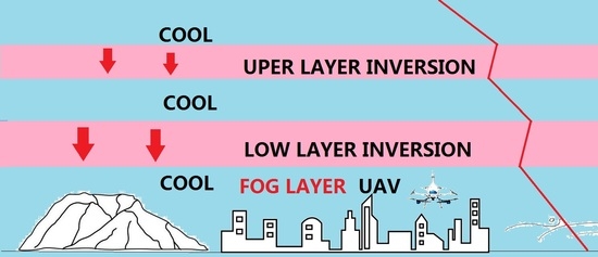
  • The double temperature inversion significantly affected the fog process, and the strengthening of the lower-level temperature inversion (from 1 to 2 °C per 100 m to 3–4 °C per 100 m) corresponded to the explosive growth of fog (the fog was quickly generated). The intensity variation in the upper-level temperature inversion affected the VIS change in the fog process. In the fog process, the bottom height of the upper-level temperature inversion layer continued to decrease, resulting in an increase in the thickness of the inversion layer. The fog process ended after the dissipation of the upper-level temperature inversion. Decreases in the VIS for the two fog processes corresponded to the strengthening of the near-surface temperature inversion, and the dissipation of fog corresponded to the weakening of the near-surface temperature inversion.
  • The thickness of the fog layer obviously affected the concentrations of air pollutants near the surface. The mass concentrations of particles decreased as the fog layer thickness increased and were maintained, while the mass concentrations of particles increased as the fog layer thickness decreased. The relationships between the changes in PM2.5 mass concentrations and the fog layer thickness were consistent for these two fog processes. The variation in PM10 mass concentrations was also related to the wind field in the boundary layer, and the downdraft had a great impact on the mass concentrations of coarse particles.
  • The thermal and dynamic conditions of the first fog process are relatively inadequate, and sufficient moisture is the main reason for the maintenance of the fog process. The boundary layer water vapor condition of the second fog process is relatively insufficient, but the deep inversion layer and weak dynamic disturbance make the fog process maintain for a long time. The maintenance of the near-surface temperature inversion with an intensity above 2 °C per 100 m contributed to the difference in the durations of the two fog processes.
By analyzing the changes in dynamic, thermal, and water vapor conditions in the atmospheric boundary layer and the mass concentration of particles in the life history of these two fog processes, it was found that the influence of meteorological conditions on different fog and haze processes was not always the same. Of course, thermal conditions were the primary conditions for the occurrence of fog processes, but water vapor conditions could determine whether or not to trigger the formation of fog. This is a conclusion that cannot be drawn only by analyzing the life history of a fog process [35,36].

Author Contributions

Conceptualization, R.L. (Ruolan Liu) and D.L.; methodology, software, D.L.; formal analysis, investigation, data curation, writing—original draft preparation, R.L. (Ruolan Liu); resources, F.Z., H.W. and R.L. (Ruixiang Liu); writing—review and editing, visualization, R.L. (Ruolan Liu), D.L. and S.Y.; validation, supervision, project administration, funding acquisition, D.L. and S.Y. All authors have read and agreed to the published version of the manuscript.

Funding

This work was jointly supported by the National Natural Science Foundation of China (42075063 and 42075066) and Natural Science Foundation of Sichuan Province (2021YJ0280), the open fund by Jiangsu Key Laboratory of Atmospheric Environment Monitoring and Pollution Control (KHK2005), and the 333 Project of Jiangsu Province, China.

Data Availability Statement

The data presented in this study are available on request from the corresponding author.

Conflicts of Interest

The authors declare no conflict of interest.

References

  1. Alizadeh-Choobari, O.; Bidokhti, A.A.; Ghafarian, P.; Najafi, M.S. Temporal and spatial variations of particulate matter and gaseous pollutants in the urban area of Tehran. Atmos. Environ. 2016, 141, 443–453. [Google Scholar] [CrossRef]
  2. Sabetghadam, S.; Alizadeh, O.; Khoshsima, M.; Pierleoni, A. Aerosol properties, trends and classification of key types over the Middle East from satellite-derived atmospheric optical data. Atmos. Environ. 2021, 246, 118100. [Google Scholar] [CrossRef]
  3. Hassan, E.M.; Alizadeh, O. Dust events in southwestern Iran: Estimation of PM10 concentration based on horizontal visibility during dust events. Int. J. Climatol. 2022, 42, 5159–5172. [Google Scholar] [CrossRef]
  4. Rangognio, J.; Tulet, P.; Bergot, T.; Gomes, L.; Thouron, O.; Leriche, M. Influence of aerosols on the formation and development of radiation fog. Atmos. Chem. Phys. Discuss. 2009, 9, 17963–18019. [Google Scholar]
  5. Zhu, Y.; Zhu, C.; Zu, F.; Wang, H.; Yuan, C.; Jiao, S.; Zhou, L. A Persistent Fog Event Involving Heavy Pollutants in Yancheng Area of Jiangsu Province. Adv. Meteorol. 2018, 2018, 2512138. [Google Scholar] [CrossRef]
  6. Yu, X.; Ma, J.; An, J.; Yuan, L.; Zhu, B.; Liu, D.; Wang, J.; Yang, Y.; Cui, H. Impacts of meteorological condition and aerosol chemical compositions on visibility impairment in Nanjing, China. J. Clean. Prod. 2016, 131, 112–120. [Google Scholar] [CrossRef]
  7. Ma, Y.; Ye, J.; Xin, J.; Zhang, W.; Vilà-Guerau de Arellano, J.; Wang, S.; Zhao, D.; Dai, L.; Ma, Y.; Wu, X.; et al. The stove, dome, and umbrella effects of atmospheric aerosol on the development of the planetary boundary layer in hazy regions. Geophys. Res. Lett. 2020, 47, e2020GL087373. [Google Scholar] [CrossRef]
  8. Ma, Y.; Xin, J.; Wang, Z.; Tian, Y.; Wu, L.; Tang, G.; Zhang, W.; Vilà-Guerau de Arellano, J.; Zhao, D.; Jia, D.; et al. How do aerosols above the residual layer affect the planetary boundary layer height? Sci. Total Environ. 2022, 814, 151953. [Google Scholar] [CrossRef]
  9. Zhao, D.; Xin, J.; Gong, C.; Quan, J.; Wang, Y.; Tang, G.; Ma, Y.; Dai, L.; Wu, X.; Liu, G.; et al. The impact threshold of the aerosol radiative forcing on the boundary layer structure in the pollution region. Atmos. Chem. Phys. 2021, 21, 5739–5753. [Google Scholar] [CrossRef]
  10. Ren, Z.H.; Yu, Y.; Han, R.; Feng, M.N. Analysis of Continuity of Fog, Light Fog and Haze Climate Series by Automatic Identification and Manual Observation. Plateau Meteorol. 2018, 37, 863–871. [Google Scholar]
  11. Wang, T.S.; Niu, S.J.; Lü, J.J.; Zhou, Y. Observational Study on the Supercooled Fog Droplet Spectrum Distribution and Icing Accumulation Mechanism in Lushan, Southeast China. Adv. Atmos. Sci. 2019, 36, 29–40. [Google Scholar] [CrossRef]
  12. Wang, H.B.; Wu, H.; Li, Y.; Xu, J.P.; Zu, F.; Zhang, Z.W. Validation of Rotorcraft UAV Boundary Layer Meteorological Observation Data and Its Application in a Heavy Fog Event in Yancheng. Meteor. Mon. 2020, 46, 89–97. [Google Scholar]
  13. Xu, W.H. Analysis of Visibility Model of PM; Pollution Based on Atmospheric Circulation. Environ. Sci. Manag. 2019, 44, 18–21. [Google Scholar]
  14. Wang, Y.; Wang, L.L.; Zhao, G.N.; Wang, Y.S.; An, J.L.; Liu, Z.R.; Tang, G.Q. Analysis of Different-Scales Circulation Patterns and Boundary Layer Structure of PM2.5 Heavy Pollutions in Beijing during Winter. Clim. Environ. Res. 2014, 19, 173–184. [Google Scholar]
  15. Chen, G.; Fang, C.H. Diagnostic analysis of a heavy fog event in November of 2009 in the south of Jiangsu province. J. Meteorol. Environ. 2011, 27, 54–57. [Google Scholar]
  16. Liu, D.Y.; Yan, W.L.; Kang, Z.M.; Liu, A.N.; Zhu, Y. Boundary-layer features and regional transport process of an extreme haze pollution event in Nanjing, China. Atmos. Pollut. Res. 2018, 9, 1088–1099. [Google Scholar] [CrossRef]
  17. Huang, H.J.; Liu, H.; Huang, J.; Mao, W.; Bi, X. Atmospheric boundary layer structure and turbulence during sea fog on the southern China coast. Mon. Weather. Rev. 2015, 143, 1907–1923. [Google Scholar] [CrossRef]
  18. Liu, D.; Yan, W.; Yang, J.; Pu, M.; Niu, S.; Li, Z. A Study of the Physical Processes of an Advection Fog Boundary Layer. Boundary-Layer. Meteorol. 2016, 158, 125–138. [Google Scholar] [CrossRef]
  19. Egli, S.; Maier, F.; Bendix, J.; Thies, B. Vertical distribution of microphysical properties in radiation fogs—A case study. Atmos. Res. 2015, 151, 130–145. [Google Scholar] [CrossRef]
  20. Li, L.; Yin, Y.; Gu, X.S.; Chen, K.; Tan, W.; Yang, L.; Yuan, L. Observational Study of Cloud Condensation Nuclei Properties at Various Altitudes of Huangshan Mountains. Chin. J. Atmos. Sci. 2014, 38, 410–420. [Google Scholar]
  21. Liu, D.; Liu, X.; Wang, H.; Li, Y.; Kang, Z.; Cao, L.; Yu, X.; Chen, H. A New Type of Haze? The December 2015 Purple (Magenta) Haze Event in Nanjing, China. Atmosphere 2017, 8, 76. [Google Scholar] [CrossRef]
  22. Xu, W.; Song, W.; Zhang, Y.; Liu, X.; Zhang, L.; Zhao, Y.; Liu, D.; Tang, A.; Yang, D.; Wang, D.; et al. Air quality improvement in a megacity: Implications from 2015 Beijing Parade Blue pollution control actions. Atmos. Chem. Phys. 2017, 17, 31–46. [Google Scholar] [CrossRef]
  23. Wu, B.G.; Zhang, H.S.; Zhang, C.C.; Zhu, H.; Wang, Z.Y.; Xie, Y.Y. Characteristics of Turbulent Transfer and Its Temporal Evolution during an Advection Fog Period in North China. Chin. J. Atmos. Sci. 2010, 34, 440–448. [Google Scholar]
  24. Zhang, E.H.; Zhu, B.; Cao, Y.C.; Wang, H.L. Analysis of the Visibility Change in the Yangtze River Delta Region in Recent 30 Years. Meteor. Mon. 2012, 38, 943–949. [Google Scholar]
  25. Zhou, Y.K.; Zhu, B.; Han, Z.W.; Pan, C.; Guo, T.; Wei, J.F.; Liu, D.Y. Analysis of visibility characteristics and connecting factors over the Yangtze River Delta Region during winter time. China Environ. Sci. 2016, 36, 660–669. [Google Scholar]
  26. Xiao, X.; Fan, S.J.; Su, R. Characteristics of a regional air pollution process over the Pearl River Delta during October 2011. Acta Sci. Circumst. 2014, 34, 290–296. [Google Scholar]
  27. Zhang, S.T.; Wang, M.J.; Liu, Y.M.; Chen, X.L.; Fan, Q. Numerical Simulation and Conceptual Model Establishment of Fogs over Pearl River Estuary, China. J. Trop. Meteorol. 2016, 32, 467–476. [Google Scholar]
  28. Zhu, Y.; Wu, Z.; Park, Y.; Fan, X.; Bai, D.; Zong, P.; Qin, B.; Cai, X.; Ahn, K.H. Measurements of atmospheric aerosol vertical distribution above North China Plain using hexacopter. Sci. Total Environ. 2019, 665, 1095–1102. [Google Scholar] [CrossRef]
  29. Shi, S.; Zhu, B.; Lu, W.; Yan, S.; Fang, C.; Liu, X.; Liu, D.; Liu, C. Estimation of radiative forcing and heating rate based on vertical observation of black carbon in Nanjing, China. Sci. Total Environ. 2021, 756, 144135. [Google Scholar] [CrossRef]
  30. Chen, Y.C.; Chang, C.C.; Chen, W.N.; Tsai, Y.J.; Chang, S.Y. Determination of the vertical profile of aerosol chemical species in the microscale urban environment. Environ. Pollut. 2018, 243, 1360–1367. [Google Scholar] [CrossRef]
  31. Liu, C.; Huang, J.; Tao, X.; Deng, L.; Fang, X.; Liu, Y.; Luo, L.; Zhang, Z.; Xiao, H.; Xiao, H. An observational study of the boundary-layer entrainment and impact of aerosol radiative effect under aerosol-polluted conditions. Atmos. Res. 2021, 250, 105348. [Google Scholar] [CrossRef]
  32. Shen, L.; Cheng, Y.; Bai, X.; Dai, H.S.; Wei, X.L.; Sun, L.S.; Yang, Y.X.; Zhang, J.S.; Feng, Y.; Li, Y.J.; et al. Vertical profile of aerosol number size distribution during a haze pollution episode in Hefei, China. Sci. Total Environ. 2022, 814, 152693. [Google Scholar] [CrossRef] [PubMed]
  33. Chen, S.; Liu, D.; Kang, Z.; Shi, Y.; Liu, M. Anomalous Atmospheric Circulation Associated with the Extremely Persistent Dense Fog Events over Eastern China in the Late Autumn of 2018. Atmosphere 2021, 12, 111. [Google Scholar] [CrossRef]
  34. Wang, B.N.; Pu, M.J.; Miao, Q. Analysis of the characteristics and variation of pollutant concentrations for a long-lasting fog and haze event in the Jiangsu area. Trans. Atmos. Sci. 2016, 39, 243–252. [Google Scholar]
  35. Sun, Y.; Zhuang, G.; Tang, A.A.; Wang, Y.; An, Z. Chemical characteristics of PM2.5 and PM10 in haze-fog episodes in Beijing. Environ. Sci. Technol. 2006, 40, 3148–3155. [Google Scholar] [CrossRef]
  36. Wu, S.; Tao, J.; Ma, N.; Kuang, Y.; Zhang, Y.; He, Y.; Sun, Y.; Xu, W.; Hong, J.; Xie, L.; et al. Particle number size distribution of PM1 and PM10 in fogs and implications on fog droplet evolutions. Atmos. Environ. 2022, 277, 119086. [Google Scholar] [CrossRef]
  37. Liu, D.Y.; Zhang, J.; Wu, X.P.; Yan, W.L.; Zhou, B.; Xie, Z.Z. Characteristics and sources of atmospheric pollutants during a fog-haze process in Huai’an. Trans. Atmos. Sci. 2014, 37, 484–492. [Google Scholar]
  38. Cui, L.K.; Song, X.Q.; Zhong, G.Q. Comparative Analysis of Three Methods for HYSPLIT Atmospheric Trajectories Clustering. Atmosphere 2021, 12, 698. [Google Scholar] [CrossRef]
  39. Shin, J.; Kim, D.; Noh, Y. Estimation of Aerosol Extinction Coefficient Using Camera Images and Application in Mass Extinction Efficiency Retrieval. Remote Sens. 2022, 14, 1224. [Google Scholar] [CrossRef]
  40. Zhang, Z.; Guo, H.; Kang, H.; Wang, J.; An, J.; Yu, X.; Lv, J.; Zhu, B. A new method for calculating average visibility from the relationship between extinction coefficient and visibility. Atmos. Meas. Tech. 2022, 15, 7259–7264. [Google Scholar] [CrossRef]
  41. GB 3095-2012; Ambient Air Quality Standards. China Environmental Science Press: Beijing, China, 2012.
  42. Qian, J.L.; Liu, D.Y.; Yan, S.Q.; Cheng, M.M.; Liao, R.W.; Niu, S.J.; Yan, W.L.; Zha, S.Y.; Wang, L.L.; Chen, X.X. Fog Scavenging of Particulate Matters in Air Pollution Events: Observation and Simulation in the Yangtze River Delta, China. Sci. Total Environ. 2023, 876, 162728. [Google Scholar] [CrossRef] [PubMed]
  43. Tian, R.Z.; Xu, J.; Zhang, Z.Z.; Tang, J.R.; Cheng, M.M. Characteristics of fog layer during heavy pollution in winter in Beijing. J. Environ. Eng. Technol. 2022, 12, 975–984. [Google Scholar]
  44. Wu, D.; Liao, B.T.; Wu, M.; Chen, H.Z.; Wang, Y.C.; Liao, X.N.; Gu, Y.; Zhang, X.L.; Zhao, X.J.; Quan, J.N.; et al. The long rerm trend of haze and fog days and the surface layer transport conditions under haze weather in North China. Acta Sci. Circumst. 2014, 34, 1–11. [Google Scholar]
Figure 1. The UAV (a) and location of UAV vertical fight operations over the city. (b) Location of province where the observation site is located; (c) Location of city where the observation site is located.
Remotesensing 15 04541 g001
Figure 2. The hourly changes in ground atmospheric horizontal visibility (unit: m), temperature (air temperature, dew point) (unit: °C), RH (%), wind direction (°), wind speed (m/s) and atmospheric particulate concentration (PM2.5, PM10) (unit: μg/m3) during the fog–haze process from 10 to 12 December 2020 in Donghai of Lianyungang, China.
Remotesensing 15 04541 g002
Figure 3. Scatter plot of RH (%) and PM concentration (unit: μg/m3) during the fog–haze process from 10 to 12 December 2020 in Donghai of Lianyungang, China.
Remotesensing 15 04541 g003
Figure 4. (a) RH (unit: %) and (b) Temperature (unit: °C) (observation by UAV) of the vertical structure evolution during the fog–haze process from 10 to 12 December 2020 in Donghai of Lianyungang, China.
Remotesensing 15 04541 g004
Figure 5. (a) The vertical structure of wind speed and (b) The temporal variation in the horizontal wind field (observation by UAV) during the fog–haze process from 10 to 12 December 2020 in Donghai of Lianyungang, China (unit: m/s). Black line: the height of the fog layer.
Remotesensing 15 04541 g005aRemotesensing 15 04541 g005b
Figure 6. The vertical profile of (a) RH (unit: %), (b) Air temperature (°C), (c) Wind speed (m/s) and (d) Wind direction (°) during the fog–haze process from 10 to 12 December 2020 in Donghai of Lianyungang, China.
Remotesensing 15 04541 g006
Figure 7. The evolutions of inversion layers and inversion intensity during the fog–haze process from 10 to 12 December 2020 in Donghai of Lianyungang, China. Bottom bar: Inversion bottom; top bar: inversion top; inversion intensity: °C/100 m. Black line: the height of the fog layer.
Remotesensing 15 04541 g007
Figure 8. The 72 h backward trajectories from 10 to 12 December in Donghai of Lianyungang, China. (a) 03:00 BJT 11 December; (b) 06:00 BJT 11 December; (c) 09:00 BJT 11 December; (d) 12:00 BJT 11 December; (e) 00:00 BJT 12 December; (f) 03:00 BJT 12 December; (g) 06:00 BJT 12 December; (h) 09:00 BJT 12 December. Red line: 10 m, Blue line: 50 m, Green line: 100 m, Cyan line: 300m, Magenta line: 500 m, Yellow line: 800 m. In the map, the horizontal ordinate is longitude, and the vertical ordinate is latitude. Asterisk is the study area.
Remotesensing 15 04541 g008
Table 1. Sensor parameters of UAV boundary layer meteorological comprehensive observation system [12]. (Type of the sensor: ZGUA-1B; company of the sensor: Nanjing Daqiao Machine Co., Ltd., Nanjing, China).
Observation ElementRange of ObservationResolutionMaximum Permissible Error
air temperature (°C)−40~400.1±0.2
RH (%)10~1001±3 (<80); ±5 (>80)
Wind speed (m/s)0.5~600.1±(0.5 + 0.03 V)
wind direction (°)0~3601±5
Table 2. The atmospheric horizontal visibility during the fog–haze event in December 2020 in Donghai.
Part NumberStarting and Ending TimeDurationFog–Haze EventThe Minimum VisibilityPM2.5 (μg/m3)PM10 (μg/m3)
(h) (m)Mean ValueRangeMean ValueRange
117:00 BJT 10–04:55 BJT 1111.9moderate haze, heavy haze1000131.5115–145172.4150–187
205:00–09:40 BJT 114.7fog4510897–128168150–209
309:41–23:45 BJT 1114.1moderate haze, heavy haze1000259.7205–206308.1253–359
423:48 BJT 11–10:30 BJT 1210.7fog42266.1196–306341.4306–390
510:31–12:00 BJT 121.5moderate haze, heavy haze1000254240–268277253–301
Disclaimer/Publisher’s Note: The statements, opinions and data contained in all publications are solely those of the individual author(s) and contributor(s) and not of MDPI and/or the editor(s). MDPI and/or the editor(s) disclaim responsibility for any injury to people or property resulting from any ideas, methods, instructions or products referred to in the content.

