Article

Spatial Downscaling of Soil Moisture Based on Fusion Methods in Complex Terrains

1
College of Atmospheric Sounding, Chengdu University of Information Technology, Chengdu 610225, China
2
Key Laboratory of Atmosphere Sounding, China Meteorological Administration, Chengdu 610225, China
3
College of Geophysics, Chengdu University of Technology, Chengdu 610059, China
4
Space Star Technology Co., Ltd., Chengdu 610199, China
5
China Satellite Network System Research Institute Co., Ltd., Beijing 100029, China
*
Author to whom correspondence should be addressed.
Remote Sens. 2023, 15(18), 4451; https://doi.org/10.3390/rs15184451
Submission received: 1 August 2023 / Revised: 1 September 2023 / Accepted: 7 September 2023 / Published: 10 September 2023
(This article belongs to the Special Issue Microwave Remote Sensing of Soil Moisture II)

Abstract

:
Large-area soil moisture (SM) data with high resolution and precision are the foundation for the research and application of hydrological and meteorological models, water resource evaluation, agricultural management, and warning of geological disasters. It is still challenging to downscale SM products in complex terrains that require fine spatial details. In this study, SM data from the Soil Moisture Active and Passive (SMAP) satellite were downscaled from 36 to 1 km in the summer and autumn of 2017 in Sichuan Province, China. Genetic-algorithm-optimized backpropagation (GABP) neural network, random forest, and convolutional neural network were applied. A fusion model between SM and longitude, latitude, elevation, slope, aspect, land-cover type, land surface temperature, normalized difference vegetation index, enhanced vegetation index, evapotranspiration, day sequence, and AM/PM was established. After downscaling, the in situ information was fused through a geographical analysis combined with a spatial interpolation to improve the quality of the downscaled SM. The comparative results show that in complex terrains, the GABP neural network better captures the soil moisture variations in both time and space domains. The GDA_Kriging method is able to merge in situ information in the downscaled SM while simultaneously maintaining the dynamic range and spatial details.

Graphical Abstract

1. Introduction

Soil moisture (SM) is a key parameter for global ecosystems [1]. It affects the energy exchange between land and atmosphere by changing conditions such as soil heat capacity, surface albedo, evapotranspiration, and vegetation [2]. SM is an essential component for delineating and forecasting agricultural droughts [3]. It can also reflect changes in mountain slopes due to heavy or long-term precipitation and predict landslides and debris flows. Accurate SM data are important in fields such as meteorology, hydrology, soil, ecology, agriculture, and environmental science.
In situ SM measurements can continuously monitor different depths of SM with a high precision and accuracy. However, the monitoring area is small with a poor spatial continuity, and the installation and maintenance are expensive. Therefore, there is no dense in situ network in many areas [4]. Nevertheless, large-area SM data are important for hydrological and meteorological modeling, agriculture, water resource management, etc. [5,6]. Remote sensing by satellites realizes the real-time observation of large-area SM, mainly by utilizing optical and microwave wavebands. Since most inversion algorithms of SM from optical wavebands are essentially empirical, the retrievals from microwave satellite systems are more reliable because of their direct measurement of energy [7]. The microwave inversion of SM mainly includes active methods based on radar or microwave scatterometers, and passive methods based on microwave radiometers [8]. Active microwave sensors have a resolution at the meter scale, but their data quantity is large and expensive with complex processing, which makes it difficult to apply. Their precision is also affected by the radar incident angle, wavelength, and polarization [9].
A passive microwave system is the main method to continuously monitor SM over extensive areas at present. Among them, the L-band is independent of solar illumination and can penetrate the atmosphere and sparse-to-medium vegetation layers to detect deeper soil signals from approximately the top 5 cm of soil layer [10]. However, passive microwave data have low spatial resolution of approximately 25–40 km due to the weak incoming energy [11]. Obtaining large-area, high-resolution, high-precision SM data by downscaling the passive microwave measurements has become a hot topic [12,13]. The downscaled results are usually interdependent in terms of the spatial distribution, detailed information, and data accuracy. According to the process mechanism and participating factors, the existing methods of passive microwave SM spatial downscaling can be divided into three different categories: the theoretical method, the spatial interpolation method, and the information fusion method. The theoretical method models the internal mechanism among physical quantities, including hydrological models [14], surface models [15] and spatial fractal models [16]. Restricted by the initial field, boundary conditions, and the complicated physical processes, it is mainly applied in small local areas. The spatial interpolation method aims to mine the spatial information connotation of coarse-scale homologous data to achieve fine-scale SM data. It performs well on simple terrains [17].
There are several factors that impact SM, and their influences are complex and nonlinear. Topography, for example, can affect the physical and chemical properties of soil, as well as the distribution of vegetation patterns on the slope [18], which leads to a spatial variation of SM. SM is negatively correlated with elevation and decreases with an increasing slope. Moreover, SM has different slopes with varying energy and duration of the receiving solar radiation. Therefore, slope and aspect directly affect material and energy distribution, soil development, vegetation types of the surface, and land-use mode, which significantly impact SM [19,20,21]. The changing topography and climate over complex terrains causes SM to shift with the evolution of the day. Furthermore, the temporal and spatial distributions of SM are influenced by various land surface environmental variables. Evapotranspiration is the main factor that affects deep soil [22]. Land surface temperature has an impact on soil evaporation, crop transpiration, and SM dynamics [23]. Vegetation canopy has the ability to intercept precipitation and decrease evapotranspiration. The understory layer can capture surface runoff and enhance surface infiltration. Vegetation roots can also form infiltration and drainage, thereby affecting water transport and SM [24]. The SM also varies with different types of land cover [25]. The information fusion method emerged as a response to these influencing variables. It is the process of combining knowledge extracted from different sensors/modalities, in order to obtain more useful or discriminant information for the purpose of regression or classification [26]. The modality is a source or form of information [27]. At present, passive microwave SM downscaling mainly fuses optical remote sensing information [28]. There are mature technologies that are easy to use, and many satellites with a high spatial resolution are available. Some researchers have used empirical polynomials to fit the downscaling relationships [29,30,31].
Some researchers have used ML methods to fuse multivariate information. Random forests [32,33,34], neural networks [13,35,36,37,38], and support vector machines [39,40] are the top three ML algorithms that have been frequently applied together with in situ SM measurements [41]. ML-based methods do not require continuous data and concurrent overpass by other satellites, but they are computationally intensive and require parameter optimization [42]. An intercomparison of different downscaling methods based on constructed synthetic datasets with a rich variability in temporal and spatial heterogeneities and patterns of SM will help to determine the applicability of each method for certain conditions [43].
There are still certain challenges regarding SM downscaling in complex terrains. The spatial and temporal heterogeneities of SM are significant due to high elevation differences, an undulating topography, messy aspects, and changing underlying surface conditions. These affect the accuracies of theoretical models [44], spatial interpolation methods [45], and empirical polynomial fittings [30]. According to the no-free-lunch theorem [46,47], different ML algorithms have different inductive preferences, which raises the question of which ML algorithm is superior for SM downscaling in complex terrains. ML models driven by data tend to move towards the sample average, weakening the extreme cases. To address these challenges, spatiotemporal information, terrain elements, land-surface environmental variables, and in situ measurements are fused to downscale SM through ML algorithms in complex terrains in this study. The genetic-algorithm-optimized backpropagation (GABP) neural network, convolutional neural network (CNN), and random forest (RF) algorithms are compared for SM downscaling in complex terrains. An in situ information fusion method based on GDA_Kriging is proposed to optimize the downscaled SM.

2. Study Area and Data

2.1. Study Area

The Tibetan Plateau, Sichuan Province of China (26.05–34.31°E, 97.35–108.54°N) is a typical “mountain-basin” area under the background of the large terrain of the Tibetan Plateau. It is located in the transition zone between the first level of the Tibetan Plateau and the second level of the Middle-Lower Yangtze plains, among the three major topographical steps of mainland China. As Figure 1 shows, there are three basic characteristics regarding the Sichuan topography: a high west and a low east undulating terrain, and complex and diverse landforms. The altitude difference between the east and west is greater than 7000 m. Plateaus, mountains, hills, plains, river valleys, rivers, and lakes are intertwined in this area, which is one of the most complex terrain areas worldwide. As shown in Figure 1a, the Hu Huanyong Line divides Sichuan into two topographical areas: the western alpine plateau and southwestern mountains, the eastern Sichuan Basin and the basin edge mountains.
The climate of Sichuan is greatly influenced by the adjacent Tibetan Plateau. Owing to the effects of atmospheric circulation, monsoon advance and retreat, and other factors, the climate of Sichuan is complex. The complex and diverse topography causes the water and heat conditions to vary greatly, resulting in large regional differences in the soil and vegetation [48]. As shown in Figure 1d, the spatial distribution of land-cover types (LCTs) in Sichuan and different climatic zones lead to changes in vegetation. The topographic features also make the landscape having a significant vertical variation [49]. Under the action of gravity and hydraulic gradients, the soil is prone to large-scale erosion. The stratigraphic lithology is complex, neotectonic movement is intense, and disasters such as earthquakes, collapses, landslides, and debris flows are frequent [50]. Heavy rains are frequent in summer, which can easily lead to meteorological and mountain geological disasters. Disasters such as droughts in autumn, heavy rain, floods, and debris flows in summer are the main environmental problems faced by Sichuan, and SM is an important limiting factor for vegetation restoration [51].

2.2. Data

In this study, the SM data included Soil Moisture Active and Passive (SMAP) satellite products for the downscaling and in situ SM data for the evaluation. Predictors were divided into land-surface environmental variables and spatiotemporal information. Land-surface environmental variables included the vegetation index (VI), land-surface temperature (LST), LCT, evapotranspiration (ET), slope, and aspect. Spatial information included longitude, latitude, and elevation, and time information referred to the day sequence and AM/PM. All the data files contained latitude, longitude, and time labels.

2.2.1. SMAP

SMAP is the first dedicated SM satellite launched by the National Aeronautics and Space Administration (NASA) that provides global maps of land-surface soil moisture and freeze–thaw state [52]. It operates in a near-polar sun-synchronous orbit of 685 km, rising at 6:00 and setting at 18:00 local solar time, covering the globe every 50 h. Its active radar failed on 7 July 2015. The passive microwave product SPL3SMP from the National Snow and Ice Data Center was used in this study. This dataset contains the L-band global 36 km EASE-Grid 2.0 surface SM, which represents the soil volumetric water content (cm3/cm3) from the top of the soil column to an average depth of approximately 5 cm [53]. Five predictors, SM, longitude, latitude, day sequence, and AM/PM, were extracted from this dataset.

2.2.2. In Situ SM

In situ observations came from the China Meteorological Administration (CMA). In situ SM in Sichuan was measured using DZN2 SM automatic observation instruments developed by China Electronics Technology Group Corporation. These instruments were developed based on the capacitive method using the principle of frequency-domain reflection. They monitor data every hour and upload data every day. Four SM elements in eight depths ranging from 0 to 100 cm underground are measured: soil volumetric water content, soil relative humidity, soil mass content, and soil water availability [54]. Soil volume water content data from 0 to 10 cm were used in this study. Sichuan Province includes 156 valid stations as marked in Figure 1b. The density of stations is sparser in the northwest, higher in the southeast, and highest in Chengdu Plain.

2.2.3. Downscaling Predictors

The elevation data in this study were obtained from the Advanced Spaceborne Thermal Emission and Reflection Radiometer GDEM V2 30 m TIFF digital elevation model (DEM) products downloaded from the Geospatial Data Cloud website of the Computer Network Information Center, Chinese Academy of Sciences. Their spatial resolution is up to 1 arcsecond horizontally and 20 m vertically [55]. Slope and aspect data were derived from the DEM.
The MODerate-resolution Imaging Spectroradiometer (MODIS) Version 6 products LST, ET, VI, and LCT were obtained from the Land Processes Distributed Active Archive Center of NASA. The LST products, MYD11A1, provided daily surface temperature and emissivity with a 1 km resolution. ET was from the evapotranspiration/latent heat flux product MOD16A2, synthesized from 8 days with a 500 m resolution. The VI product MOD13A2 was synthesized for 16 days with a 1 km resolution. The normalized difference vegetation index (NDVI) and enhanced vegetation index (EVI) were used. The LCT annual product, MCD12Q1, had a resolution of 500 m. The International Geosphere-Biosphere Programme was used in this study, including 17 types. The variable types, sources, spatiotemporal resolutions, and data units for this study are listed in Table 1.

3. Methodology

High-resolution features were first upscaled to 36 km to match with the 36 km SMAP in time and space. The unified 36 km source and target data composed the training and validation sets for model training. The downscaling of SM was achieved by feeding 1 km predictors to the models trained with the 36 km data [13,29]. A flowchart of this study is shown in Figure 2, including the data processing, downscaling fusion, and in situ SM fusion.
The data preprocessing procedure was used to generate a 36 km training and validation set and a 1 km test set through spatiotemporal matching. The two key steps in the preprocessing procedure were data structuring and spatiotemporal matching. Data structuring converted the data into csv files whose columns were longitude, latitude, and variable values through data stitching, unification of projection, coordinate system transformation, resampling, clipping, and sorting. Both time matching and space matching utilized the nearest neighbor method to match different variables. Time matching took SMAP as the benchmark after the time of all kinds of data were uniformed to Coordinated Universal Time. Since there was no SMAP in the test set, LST was taken as the benchmark. Space matching used the coarse scale variable as the benchmark. In this study, the summer and autumn of 2017 and Sichuan Province were used as the experimental time and space. After data preprocessing, 8670 samples on a coarse scale of 36 km were obtained. The validation set was randomly selected from 30% of these samples.
In the downscaling fusion, ML algorithms were used to train the samples. The GABP neural network optimized itself in two ways. First, it used the fitness function as the optimization index to find the optimal initial weights, thresholds, and number of hidden layer neurons through the genetic algorithm. Second, it optimized the weights of each layer through error backpropagation until the target accuracy was achieved. A CNN can extract abstract features and reduce complexity through weight-sharing (convolution) and downsampling (pooling) strategies. Its model parameters can be trained using the gradient descent method. Researchers have used CNN models to achieve the super-resolution reconstruction of remote sensing images [56,57]. An RF integrates multiple independent decision trees based on two different random processes: sample disturbance and feature disturbance. The RF regression model considers multiple independent variables as affecting the dependent variable.
After tuning the hyperparameters and learning curves, the optimal models for the GABP neural network, CNN, and RF methods were obtained. The optimal GABP neural network model consisted of a three-layer network. The tansig activation function was used in the hidden layer, and the purelin function was used in the output layer. Trainlm was chosen as the training function, which is suitable for small- and medium-sized networks and has a faster convergence. Additionally, multiple tests were conducted to determine other parameters. The initial population size was 100, the roulette method was used for the gene selection, the learning rate was set to 0.05, and the target accuracy was a mean square error (MSE) of 0.001 m3/m3. Genetic algorithms consist of three important parameters: chromosome structure, gene coding, and fitness function. In this study, the chromosome structure included the weight and threshold of each layer and the number of neurons in the hidden layer. Real number coding was used for gene coding because its data are the weights and thresholds themselves, which are suitable for continuous data. Arithmetic crossover was chosen because it is well-suited for real encoding. The nonuniform mutation method was selected after comparing it to multiple widely used methods. The crossover probability and mutation probability were adjusted based on the fitness value of individuals. The reciprocal of the sum of squared errors was used as the fitness function according to the problem addressed in this study. The population evolved for 4000 generations according to the fitness function curves of the genetic algorithm. However, maximum fitness was reached and stayed stable after 262 generations. Considering the network accuracy and efficiency, the 262nd-generation parameters were used as the optimal initial weight, threshold, and number of hidden layer neurons. The fitness of this model was 0.27, the R2 of the validation set was 0.76, and the average absolute error was 0.03 m3/m3.
The CNN was implemented using Python3.6 GPU Keras 2.4.3. According to the model complexity theory [58], the neural network’s best fitting was obtained when the errors of both the training set and validation set were very low. Through drawing the 1500-epoch training curves, the best fitting was at the 570th epoch. The validation set reached the minimum mean absolute error (MAE) (0.0355 m3/m3), and the MAE (0.0349 m3/m3) of the training set was also very low. In the optimal model, four groups of convolutional layers were designed to learn higher-level features, and each group included two one-dimensional convolutional layers, a maximum pooling layer, and a dropout layer. Adam and MSE were used as the optimization function and loss function, respectively. RF was modeled using RandomForestRegressor from Python’s Sklearn package. A grid search and 20-fold cross-validation were used for hyperparameter tuning. The optimal model parameters were obtained according to the MSE.
The 1 km test set was imported into the three models for prediction, and the 1 km downscaled results were obtained, which are hereafter referred to as “GABP”, “CNN”, and “RF”, respectively. SMAP SM and in situ SM were used to compare the three results from the statistical, temporal, and spatial distributions.
In the fusion step, the in situ SM and high-resolution SM (HRSM) data were preprocessed by eliminating systematic errors and spatiotemporal matching. The error was expanded from the point scale to the fine-grid scale by geospatial interpolation. The downscaled results and in situ information fusion were realized by a geographic analysis, which is a nonparametric data fusion method based on error. It is often used to calibrate satellite data from ground-measured data and usually includes a geographical difference analysis (GDA) and geographical ratio analysis (GRA) [59]. The neighboring in situ stations were used to correct the background field by determining the weight of the in situ points at the interpolation point to estimate the error field. Finally, the fusion field is the sum or product of the error and the background fields. Equations (1) and (2) describe the fusion process based on the addition and multiplication errors, respectively. The error estimate of position i, e ^ HRSM ( i ) or r ^ HRSM ( i ) , was the sum of the error weights of k neighboring stations FSitu. The weight Wj was obtained by the Kriging or inverse distance weight (IDW) spatial interpolation method [60], and its corresponding fusion field F ^ ( i ) was the sum or product of the error estimate and background field FHRSM.
F ( i ) ^ = F HRSM ( i ) + e ^ HRSM ( i ) e ^ HRSM ( i ) = j = 1 k W j F Situ ( j ) F HRSM ( j )
F ^ ( i ) = F HRSM ( i ) × r ^ HRSM ( i ) r ^ HRSM ( i ) = j = 1 k W j F Situ ( j ) / F HRSM ( j )
In the evaluation step, the root-mean-square error (RMSE), MAE, and Pearson correlation coefficient (CC) methods were used, as shown in Equations (3)–(5), where Xi refers to the evaluation data, and Yi refers to the estimated data.
R M S E = 1 n i = 1 n X i Y i 2
M A E = 1 n i = 1 n X i Y i .
C C = i = 1 n X i X ¯ Y i Y ¯ i = 1 n X i X ¯ 2 i = 1 n Y i Y ¯ 2

4. Results and Analysis

4.1. Correlation Analysis of Model Variables

To analyze the correlation between SM and its predictors in different seasons and areas, the training set was divided into summer and autumn seasons. It was also divided into northwest (NW) and southeast (SE) areas based on a 3000 m elevation threshold, as shown in Figure 1a. The sample sizes for Total, summer, autumn, NW, and SE were 8670, 3465, 5025, 4219, and 4451, respectively. Figure 3 displays bar (a) and stacked bar (b) plots for the CC analysis. The stacked bars ignore the positive and negative CCs, and CCs with p-values more than 0.05 are in black. Figure 3 shows the following: (1) in the total set as shown in Figure 3a, all CCs except for the slope passed the significance test with a 95% confidence interval. Elevation, slope, and day sequence had large negative correlations with SM. The remaining predictors were positively correlated with SM, and the CCs from high to low were longitude, LST, EVI, ET, LCT, latitude, AM/PM, and NDVI. Although some predictors had low CCs, they would also work in nonlinear models. (2) The largest contributing factors were slope, elevation, day sequence, and longitude. These factors had the top four CCs in the total set and the subset, indicating that terrain and spatiotemporal information had a significant impact. Day sequence, ET, latitude, LST, and EVI were more effective in autumn than in summer and in the NW area than in the SE area. (3) In autumn, all p-values were less than 0.05. In summer, the p-values of several variables exceeded 0.05. Except for the slope, elevation, and day sequence, the LCT, AM/PM, and aspect were influential in summer, while others had low CCs. (4) Regionally, most of the CCs were relatively high in the NW area. In the SE area, predictors had little or no influence except for the elevation, longitude, and slope. (5) The EVI was a better representation of vegetation effects than the NDVI. The EVI and NDVI were more influential in autumn than in summer. The aspect had a greater influence in the NW area than in the SE area. Figure 3c shows the importance of each predictor in the RF model from high to low. It can be seen that the predictors with the highest impact were elevation, day sequence, latitude, longitude, and slope, and the impact degrees of these five features were much higher than those of the others. Thus, the SM downscaling in complex terrains should include the spatiotemporal information and terrains as inputs.

4.2. Comparisons of the Downscaled Results

Ground evaluation is a key step before utilizing satellite inversion data. Boxplots (Figure 4a) and probability density function (PDF) curves (Figure 4b) were used to compare the statistical distribution of the five SM datasets of in situ SM, the original SMAP, GABP, RF, and CNN in Sichuan Province during the summer and autumn of 2017. The sample sizes of the first two were 45,364 and 8670, and those of the latter three were 15, 937, and 221. The in situ SM can be measured in all weather and every day with a larger range. The measurement depth is different between the satellite (5 cm) and in situ SM (10 cm). As shown in Figure 4a, the data range is reduced from left to right. GABP was more consistent with SMAP than with the RF and CNN. GABP maintained the dynamic range and mean level of SMAP, whereas the RF and CNN reduced the dynamic range. As shown in Figure 4b, GABP and SMAP had the best consistence among these curves. SMAP data showed an obvious normal distribution. The RF and CNN data distributions were more concentrated and showed two or more peaks, which were quite different from that of SMAP. The in situ SM had a wider distribution and higher average. The main reasons were as follows: Because of the gravity infiltration of soil water and the evaporation of surface water, in situ measurements (10 cm) contain more water than SMAP (5 cm); in situ measurements contain data during cloud and rain weather; the stations are denser in the southeast and sparser in northwest Sichuan. Moreover, the southeast area has a stronger water-holding capacity because the terrain is low-lying and the vegetation is dominated by woody savannas, savannas, cropland/natural vegetation mosaics, evergreen broadleaf forests, and deciduous broadleaf forests.
In the following section, the results from the three ML methods are compared in the time and space domains. After time and space matching, the sample numbers of SMAP were 3092, 1247, and 1845 in total, summer, and autumn, respectively, and those of GABP (RF or CNN) were 4904, 1911, and 2933. In situ SM and the four datasets both excluded cloud and rain areas, invalid value areas, unscanned areas, and low-precision SMAP areas such as ice, snow, water bodies, and bare ground. MAEs were used to analyze the differences in the time domain. Figure 5 shows the bars of monthly, seasonal, and total MAEs of the SMAP, GABP, RF, and CNN SM relative to the in situ SM. It can be seen that the MAE of the downscaled results was generally better than that of SMAP, in which GABP had the lowest and the CNN had the highest MAE. The MAE was significantly higher for the CNN in autumn and slightly higher for the RF in summer. The four datasets were more accurate in autumn than in summer, with August having the highest MAE and GABP and RF having the lowest MAE in September. This may be attributed to the abrupt changes of SM with heavy precipitation during the summer. In summer, the MAEs of GABP were much lower than those of the RF and CNN, indicating that GABP was better able to capture abrupt variations in the time domain.
Figure 6 shows the spatial distributions of the mean SM of the in situ SM (a), GABP (b), RF (c), CNN (d), and SMAP (e) data in Sichuan during the summer and autumn of 2017. The downscaled results of the GABP network, RF, and CNN in the red-box region of Figure 6e are enlarged in Figure 6f–h, respectively. As can be seen from Figure 6, the five distributions were all wet in the southeast and dry in the northwest. However, the northwest boundary areas became wet. The in situ data were wetter, but the spatial variation trend was consistent with the others. The three downscaled results showed the spatial heterogeneity of SM, which was absent in the original 36 km SMAP data because of their coarse spatial resolution.
As shown in Figure 6b, among the three downscaled SM datasets, GABP has a wider dynamic range, which can more accurately depict the spatial distribution of the SMAP and provide a finer spatial variability. The texture features presented by the GABP SM clearly show topographic changes, such as mountain elevation and slope. In the low-lying and flat Sichuan Basin, all three models can represent the spatial distribution of SMAP. In the Western Sichuan Plateau and the transition zone with large topographic fluctuations, GABP shows clear advantages in terms of data consistency and detail representation, which can better retain the spatial distribution and quality of SMAP. In Figure 6c, the distribution of the RF is also consistent with SMAP, but it shows abrupt changes at some longitudes and latitudes. By analyzing the importance values of the RF model (Figure 2b), the large influence of the longitude and latitude makes the regression trees show obvious differences in inductive preferences on both sides of some longitude and latitude lines, because the longitude and latitude values show an isometric monotonic increase in space. In Figure 6d, the CNN also has a similar spatial variation to SMAP, but both are too smooth, and the heterogeneous information is far less than that of GABP and the RF. The CNN algorithm fuses the neighborhood information through spatial convolution, but the training set at a scale of 36 km has less effective correlation information, which smooths the local features. Therefore, the CNN model has limitations when applied to spatial downscaling. As shown in Figure 6f–h, the transitional zone from the Sichuan Basin to the Western Sichuan Plateau increases sharply. The downscaled results of the GABP neural network shown in Figure 6f can more accurately represent the fluctuation of SM with topography and mountain texture, and it can overcome the sudden changes in the longitude and latitude of the RF in Figure 6g and the spatial smoothness of the CNN in Figure 6h.
In conclusion, the GABP neural network method shows a more accurate feature expression in SM downscaling in complex terrains in this study. This is because most of the CCs of predictors are relatively high in the NW area, and predictors have little or no influence except for elevation, longitude, and slope in the SE area as Figure 3b shows. The GABP neural network can self-adjust parameters, self-evolve, and self-adapt, making it more accurate in describing complex relationships. This study is a regression problem, and the basis of a neural network is a multisource nonlinear regression. RFs, on the other hand, are essentially decision trees that are more suitable for classification scenarios. For regression problems, they are based on the average of multiple decision trees. A CNN captures spatial relationships in the adjacent area. However, since the training set is 36 km in space, it is too coarse to transfer this relationship to 1 km.

4.3. In Situ SM Fusion Results

To improve the data quality, high-precision but sparse ground measures were incorporated into the downscaled results. The spatial distribution of in situ SM is shown in Figure 6a. In this experiment, the 1 km GABP-downscaled results were used as the calibration object (the HRSM). Thirty percent of the in situ data were randomly selected for verification, which were not involved in the fusion process. The RMSE and MAE were used as the verification scores. As Table 2 shows, the results of the in situ SM fusion were all better than those of the prefusion HRSM. The IDW interpolation had a smaller RMSE and MAE than the Kriging interpolation. For the same interpolation, the GDA was better than the GRA, with a smaller RMSE and MAE.
In the following, the two datasets before fusion (HRSM and in situ SM) and the four fusion results, GDA_Kriging, GRA_Kriging, GDA_IDW and GRA_IDW, were compared using boxplots (Figure 7a) and PDFs (Figure 7b). The in situ data shown here only include those that had undergone spatiotemporal matching.The boxplots and PDFs show that the in situ data had the highest mean score. In terms of the dynamic range, the in situ data were the widest, the two IDW results were narrower, and the two Kriging results and HRSM were similar. The PDF curves for the two Kriging results resembled HRSM more closely. When using the same interpolation method, the GRA result was slightly higher than that of the GDA. In general, the Kriging method could better preserve the dynamic range and statistical characteristics of the HRSM during fusion.
Although the result of the GDA was slightly better than that of the GRA, the following only compares GDA_Kring and GDA_IDW because the GDA was unable to compute the ratio (X/0). Figure 8 shows the daily average sequence curves for in situ SM, HRSM, GDA_Kriging, and GDA_IDW. As can be seen from Figure 8, relative to HRSM, the fusion data have a greater variation, and the change trend coincides with the in situ data, especially in summer. This indicates that the fusion results contain in situ information and tend toward the in situ information. This method can realize data fusion and correction at the same time and improve the dynamic ranges of spatial averages.
To compare and analyze the spatial distribution of the data before and after fusion, the spatial distributions of the mean SMs for HRSM, GDA_Kriging, and GDA_IDW are shown in Figure 9. As shown in Figure 9, the Kriging method retains the spatial variation details of HRSM and simultaneously fuses the in situ information, but there are point mutations at the station locations. The IDW method smooths the mutations at stations, but also smooths the spatial variations of HRSM, loses some extreme values, and narrows the data range. Therefore, the Kriging method can retain the spatial variation details of the HRSM and dynamic range of the site better than the IDW method.

5. Discussion and Conclusions

Obtaining large-area data with a high resolution and precision is a bottleneck in SM remote sensing. In complex terrains, SM is more spatially heterogeneous and fine-scale SM data are required. This study explored the SM spatial downscaling and information fusion methods suitable for complex terrains. Three ML algorithms, a GABP neural network, an RF, and a CNN, were compared by fusing multiple factors, and in situ SM data were fused into the downscaled results by way of a GDA combined with a spatial interpolation. The main conclusions are as follows:
(1)
Themost correlated predictors were slope, elevation, day sequence, and longitude. The day sequence, ET, latitude, LST, and EVI were more effective in autumn than in summer and in the NW area than in the SE area. Most of the CCs were relatively high in the NW area. The EVI was a more effective indicator of vegetation than the NDVI. The aspect was more effective in the NW area than in the SE area. The elevation, day sequence, latitude, longitude, and slope had a much higher importance than the other predictors in the RF model. It is important to include spatiotemporal information and terrain as inputs in downscaling SM over complex terrains.
(2)
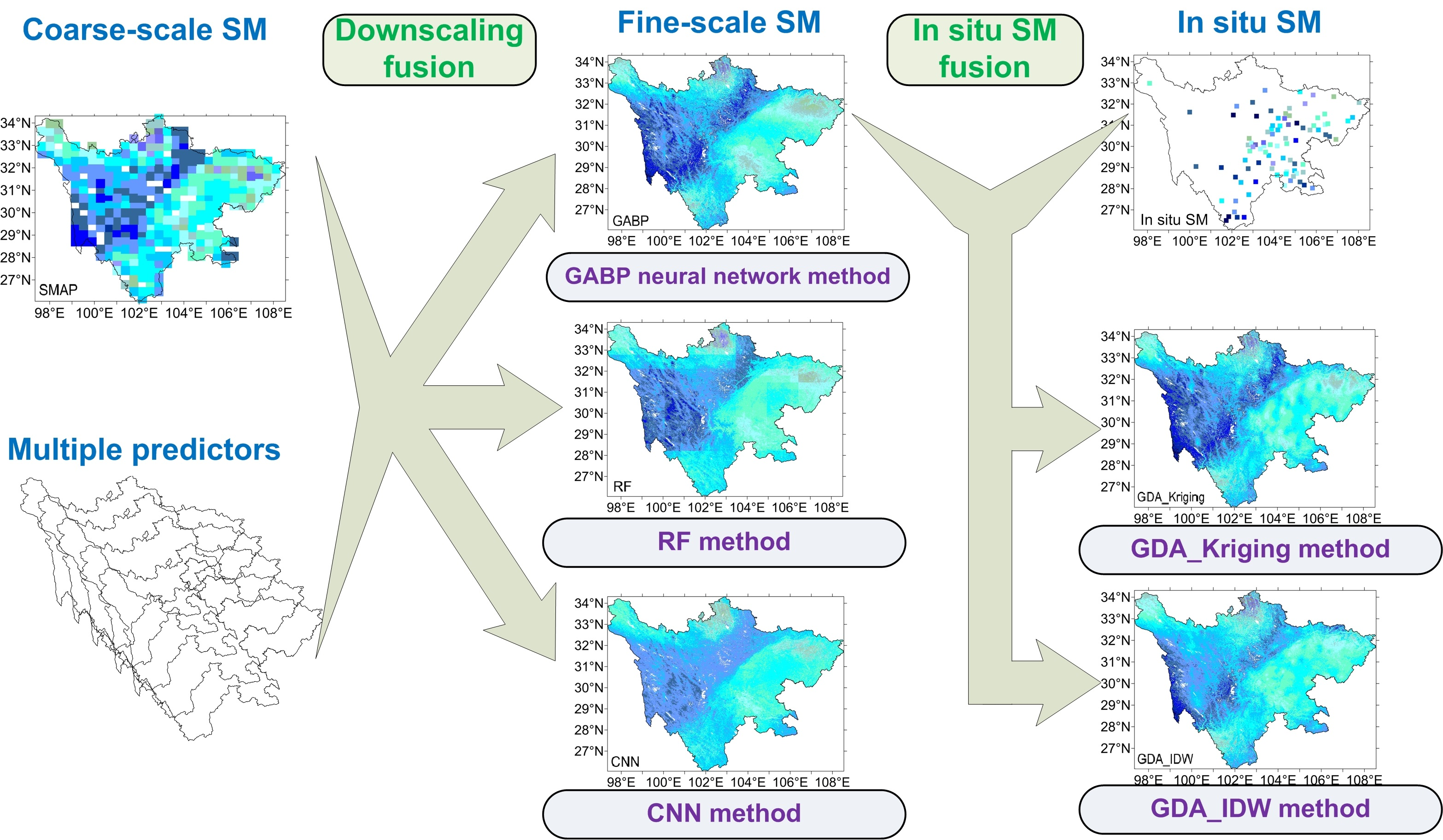
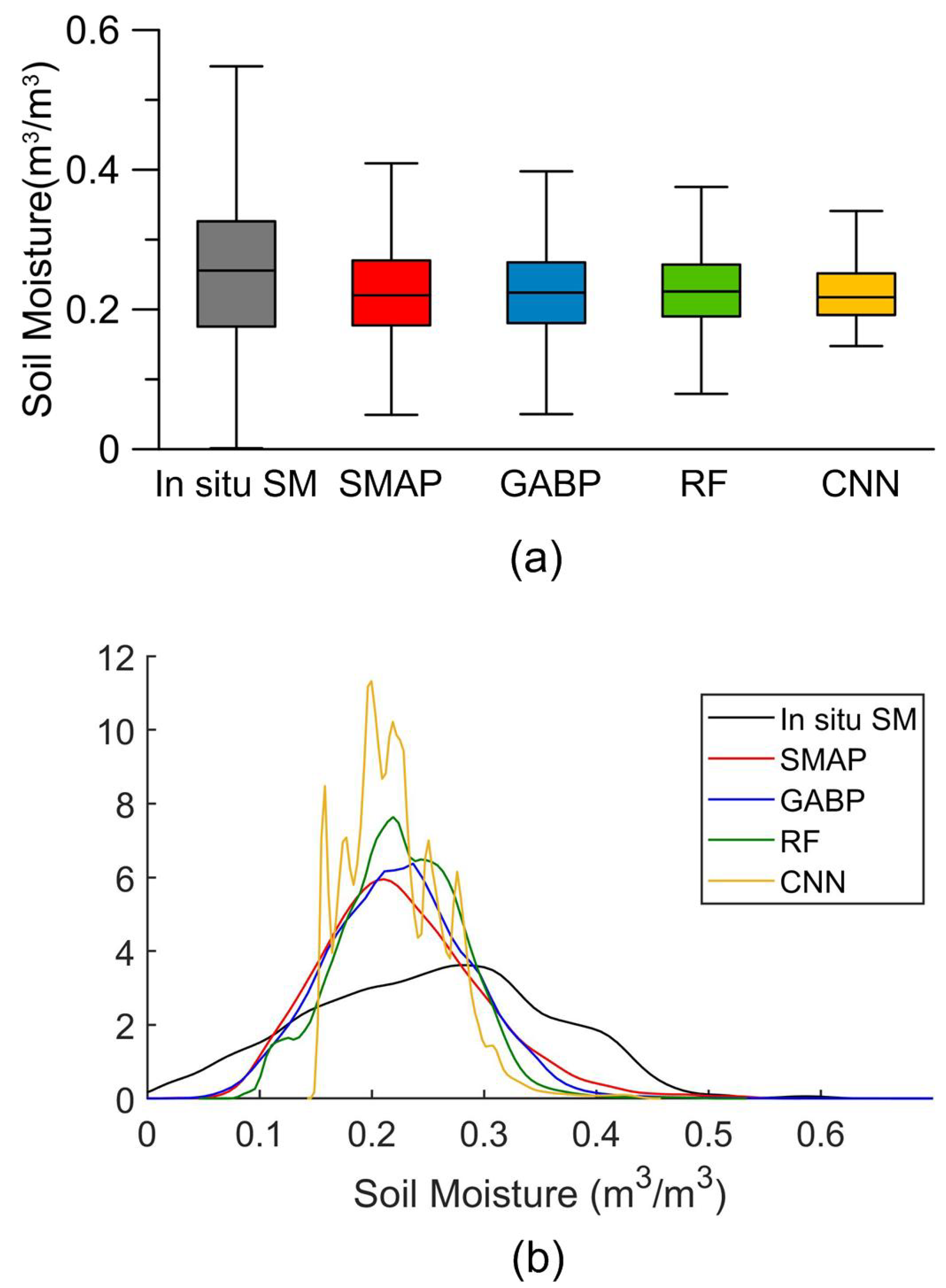
The GABP neural network showed advantages in data accuracy and spatial and temporal fineness when compared to the RF and CNN. The GABP neural network results maintained the dynamic range and mean level of the original SMAP with statistical consistency, whereas the RF and CNN reduced the dynamic range. These three methods could reduce the error of SMAP, and the data were more accurate in autumn than in summer. The GABP neural network had the smallest error among the three, especially in summer. RF was prone to abrupt warp and weft changes in space, and the CNN had a spatial smoothness. The GABP neural network model can better capture the mean states and details of variation in time and space, and it has advantages in high-elevation areas and large undulating terrains over the RF and CNN.
(3)
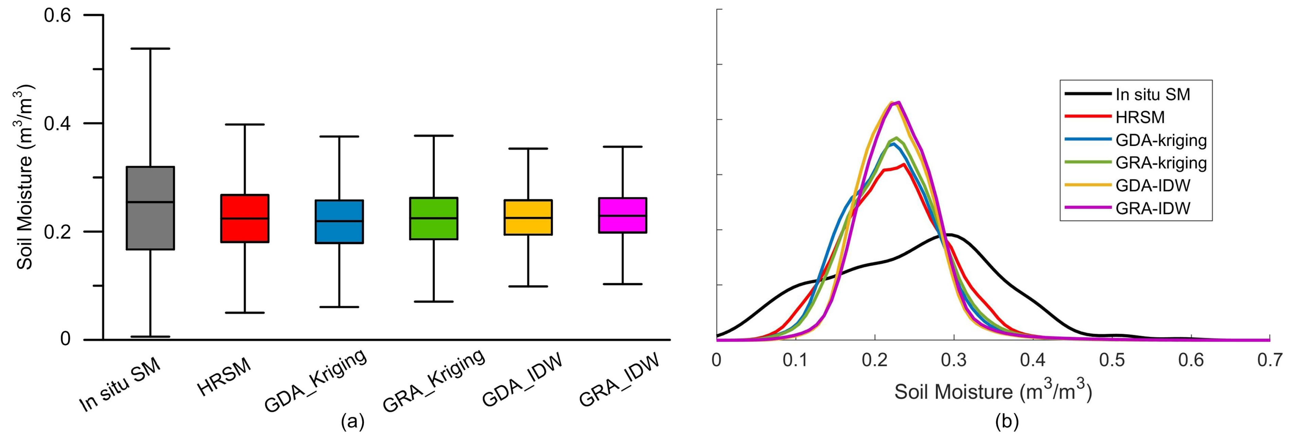
In the in situ SM fusion, the GDA had a lower RMSE and MAE than the GRA when applying the same interpolation method. The GDA_Kriging interpolation method could better preserve the dynamic range, statistical characteristics, and spatial details of the HRSM data than the GDA_IDW method. The fusion results improved the dynamic range of the HRSM and was closer to the in situ SM. The GDA_IDW method tended to smooth the spatial variations.
Despite the aforementioned contributions, this study still has the following limitations: (1) ML is often considered a black box that is difficult to explain and verify in terms of physical mechanisms. In future studies, physical models can be combined with ML models. Physics can be used to design loss functions [41,61], initialize auxiliary models, structure design models, model residual errors, and create hybrid models [62]. Incorporating physical constraints and partial prior knowledge into the optimization direction and network structure can better utilize limited data resources, leading to improved model accuracy and design effectiveness [63]. (2) The LST data in this study were obtained from MODIS’s thermal infrared remote sensing, which has a high spatial and temporal resolution and inversion accuracy. However, because of the influence of clouds, this method is only applicable to cloud-free areas. (3) The training set did not include cloud areas, and the SMAP products exhibit a “dry bias” in high, cold mountainous areas [4]. Therefore, the downscaled results were lower than the in situ SM, and the model is more suitable for low SM situations. (4) When the SM is downscaled to the same fine spatial resolution, there will be more redundant information in flat areas. In future studies, the spatial scale should be adjusted adaptively according to terrain complexity. The change degree of elevation, slope, aspect, and LCT can be used as an index to adaptively adjust the spatial resolution of the inversion data. (5) This study was based on the assumption that the scale of the model relationship was constant, and spatial information difference was used to reduce the impact of spatial heterogeneity. The downscaling methods presented in this study have potential applications for other elements that have downscaling requirements in complex terrains, such as precipitation, temperature, radiation, and wind speed.

Author Contributions

Conceptualization, Q.C., X.T. and F.M.; methodology, Q.C. and X.T.; software, B.L. and G.S.; validation, Q.C., B.L. and Z.T.; formal analysis, H.W. and Q.Z.; investigation, G.S.; resources, Z.T. and L.Y.; data curation, H.W. and Q.Z.; writing—original draft preparation, Q.C.; writing—review and editing, Q.C. and X.T.; visualization, Q.C.; supervision, F.M.; project administration, Q.C.; funding acquisition, L.Y., H.W. and Q.Z. All authors have read and agreed to the published version of the manuscript.

Funding

This research was funded by the Project of the Sichuan Department of Science and Technology (2022NSFSC0216).

Data Availability Statement

Publicly available datasets were used in this study. This data can be found here: (1) DEM dataset can be obtained at http://www.gscloud.cn/ (accessed on 1 November 2021). (2) SMAP dataset can be obtained at https://nsidc.org/data/SPL3SMP/versions/5 (accessed on 1 November 2021). (3) MODIS dataset can be obtained at https://e4ftl01.cr.usgs.gov/MOLA/ (accessed on 1 November 2021). In situ SM are provided by the China Meteorological Administration and belong to non-public data. Regarding the datasets generated during and/or analyzed during the current study are available from the corresponding author on reasonable request.

Acknowledgments

We would like to express our sincere thanks to the China Meteorological Administration, Geospatial Data Cloud Platform of Computer Network Information Center of Chinese Academy of Sciences, National Snow and Ice Data Center, and Land Processes Distributed Active Archive Center for supplying the data and the reviewers for their constructive comments and editorial suggestions that helped improve the quality of the manuscript.

Conflicts of Interest

The authors declare no conflict of interest.

References

  1. Islam, S.; Engman, T. Why bother for 0.0001% of Earth’s water? Challenges for soil moisture research. Eos Trans. Am. Geophys. Union 1996, 77, 420. [Google Scholar] [CrossRef]
  2. Gao, C.; Li, G.; Xu, B.; Li, X. Effect of spring soil moisture over the Indo-China Peninsula on the following summer extreme precipitation events over the Yangtze River basin. Clim. Dyn. 2020, 54, 3845–3861. [Google Scholar] [CrossRef]
  3. Chatterjee, S.; Desai, A.R.; Zhu, J.; Townsend, P.A.; Huang, J. Soil moisture as an essential component for delineating and forecasting agricultural rather than meteorological drought. Remote Sens. Environ. 2022, 269, 112833. [Google Scholar] [CrossRef]
  4. Zhang, L.; He, C.; Zhang, M.; Zhu, Y. Evaluation of the SMOS and SMAP soil moisture products under different vegetation types against two sparse in situ networks over arid mountainous watersheds, Northwest China. Sci. China Earth Sci. 2019, 62, 703–718. [Google Scholar] [CrossRef]
  5. Wakigar, S.A.; Leconte, R. Exploring the utility of the downscaled SMAP soil moisture products in improving streamflow simulation. J. Hydrol. Reg. Stud. 2023, 477, 101391. [Google Scholar] [CrossRef]
  6. Fang, B.; Kansara, P.; Dandridge, C.; Lakshmi, V. Drought monitoring using high spatial resolution soil moisture data over Australia in 2015–2019. J. Hydrol. 2021, 594, 125960. [Google Scholar] [CrossRef]
  7. Schmugge, T. Remote Sensing of Surface Soil Moisture. J. Appl. Meteorol. 1978, 17, 1549–1557. [Google Scholar] [CrossRef]
  8. Draper, C.S.; Reichle, R.H.; De Lannoy, G.J.M.; Liu, Q. Assimilation of passive and active microwave soil moisture retrievals. Geophys. Res. Lett. 2012, 39, 194. [Google Scholar] [CrossRef]
  9. Toride, T.; Sawada, Y.; Aida, K.; Koike, T. Toward High-Resolution Soil Moisture Monitoring by Combining Active-Passive Microwave and Optical Vegetation Remote Sensing Products with Land Surface Model. Sensors 2019, 19, 3924. [Google Scholar] [CrossRef] [PubMed]
  10. Entekhabi, D.; Njoku, E.G.; O’Neill, P.E.; Kellogg, K.H.; Crow, W.T.; Edelstein, W.N.; Entin, J.K.; Goodman, S.D.; Jackson, T.J.; Johnson, J.; et al. The Soil Moisture Active Passive (SMAP) mission. Proc. IEEE 2010, 98, 704–716. [Google Scholar] [CrossRef]
  11. Ma, H.; Zeng, J.; Chen, N.; Zhang, X.; Cosh, M.H.; Wang, W. Satellite surface soil moisture from SMAP, SMOS, AMSR2 and ESA CCI: A comprehensive assessment using global ground-based observations. Remote Sens. Environ. 2019, 231, 111215. [Google Scholar] [CrossRef]
  12. Zhang, X.; Dong, J.; Huang, S.; Nam, W.; Niyogi, D.; Xu, L.; Chen, N.; Fu, P.; Gu, X.; Rab, G. A novel fusion method for generating surface soil moisture data with high accuracy, high spatial resolution, and high spatio-temporal continuity. Water Resour. Res. 2022, 58, e2021WR030827. [Google Scholar] [CrossRef]
  13. Lv, A.; Zhang, Z.; Zhu, H. A Neural-Network Based Spatial Resolution Downscaling Method for Soil Moisture: Case Study of Qinghai Province. Remote Sens. 2021, 13, 1583. [Google Scholar] [CrossRef]
  14. Yang, H.; Xiong, L.; Liu, D.; Cheng, L.; Chen, J. High spatial resolution simulation of profile soil moisture by assimilating multi-source remote-sensed information into a distributed hydrological model. J. Hydrol. 2021, 597, 126311. [Google Scholar] [CrossRef]
  15. Rouf, T.; Maggioni, V.; Mei, Y.; Houser, P. Towards hyper-resolution land-surface modeling of surface and root zone soil moisture. J. Hydrol. 2021, 594, 125945. [Google Scholar] [CrossRef]
  16. Kwon, M.; Kwon, H.-H.; Han, D. A Spatial Downscaling of Soil Moisture from Rainfall, Temperature, and AMSR2 Using a Gaussian-Mixture Nonstationary Hidden Markov Model. J. Hydrol. 2018, 13, 1583. [Google Scholar] [CrossRef]
  17. Chan, S.K.; Bindlish, R.; O’Neill, P.; Jackson, T.; Njoku, E.; Dunbar, S.; Chaubell, J.; Piepmeier, J.; Yueh, S.; Entekhabi, D.; et al. Development and assessment of the SMAP enhanced passive soil moisture product. Remote Sens. Environ. 2017, 204, 931–941. [Google Scholar] [CrossRef] [PubMed]
  18. Vinnikov, K.Y.; Robock, A.; Speranskaya, N.A.; Schlosser, C.A. Scales of temporal and spatial variability of midlatitude soil moisture. J. Geophys. Res. 1996, 101, 7163–7174. [Google Scholar] [CrossRef]
  19. Qiu, Y.; Fu, B.; Wang, J.; Chen, L. Soil moisture variation in relation to topography and land use in a hillslope catchment of the Loess Plateau, China. J. Hydrol. 2001, 240, 243–263. [Google Scholar] [CrossRef]
  20. Lei, F.; Wade, C.; Shen, H.; Robert, P.; Thomas, H. The Impact of Local Acquisition Time on the Accuracy of Microwave Surface Soil Moisture Retrievals over the Contiguous United States. Remote Sens. 2015, 7, 13448–13465. [Google Scholar] [CrossRef]
  21. Parinussa, R.M.; Holmes, T.; Crow, W.T. The impact of land surface temperature on soil moisture anomaly detection from passive microwave observations. Hydrol. Earth Syst. Sci. Discuss. 2011, 8, 3135–3151. [Google Scholar] [CrossRef]
  22. Teuling, A.J.; Seneviratne, S.I.; Williams, C.; Troch, P.A. Observed timescales of evapotranspiration response to soil moisture. Geophys. Res. Lett. 2006, 33, L23403. [Google Scholar] [CrossRef]
  23. Zhao, S.; Yang, Y.; Qiu, G.; Qin, Q.; Yao, Y.; Xiong, Y.; Li, C. Remote detection of bare soil moisture using a surface-temperature-based soil evaporation transfer coefficient. Int. J. Appl. Earth Obs. Geoinf. 2010, 12, 351–358. [Google Scholar] [CrossRef]
  24. Liu, S.; Liu, S.; Fu, Z.; Sun, L. A nonlinear coupled soil moisture-vegetation model. Adv. Atmos. Sci. 2005, 22, 337–342. [Google Scholar] [CrossRef]
  25. Francis, C.F.; Thornes, J.B.; Romero Diaz, A.; Lopez Bermudez, F.; Fisher, G.C. Topographic control of soil moisture, vegetation cover and land degradation in a moisture stressed mediterranean environment. Catena 1986, 13, 211–225. [Google Scholar] [CrossRef]
  26. Guan, L.; Gao, L.; Din, E.N.; Liang, C. Statistical Machine Learning vs Deep Learning in Information Fusion: Competition or Collaboration? In Proceedings of the 2018 IEEE Conference on Multimedia Information Processing and Retrieval (MIPR), Miami, FL, USA, 10–12 April 2018; pp. 251–256. [Google Scholar] [CrossRef]
  27. Sun, X.; Tian, Y.; Lu, W.; Wang, P.; Niu, R.; Yu, H.; Fu, K. From single- to multi-modal remote sensing imagery interpretation: A survey and taxonomy. Sci. China Inf. Sci. 2023, 66, 140301. [Google Scholar] [CrossRef]
  28. Song, P.; Zhang, Y.; Tian, J. Improving surface soil moisture estimates in humid regions by an enhanced remote sensing technique. Geophys. Res. Lett. 2021, 48, e2020GL091459. [Google Scholar] [CrossRef]
  29. Zhao, W.; Wen, F.; Wang, Q.; Sanchez, N.; Piles, M. Seamless downscaling of the ESA CCI soil moisture data at the daily scale with MODIS land products. J. Hydrol. 2021, 603, 126930. [Google Scholar] [CrossRef]
  30. Chen, Q.; Miao, F.; Xu, Z.-X.; Wang, H.; Yang, L.; Tang, Z. Downscaling of Remote Sensing Soil Moisture Products Based on TVDI in Complex Terrain Areas. In Proceedings of the International Conference on Meteorology Observations (ICMO), Chengdu, China, 28–31 December 2019. [Google Scholar] [CrossRef]
  31. Ojha, N.; Merlin, O.; Molero, B.; Suere, C.; Olivera-Guerra, L.; Hssaine, A.B.; Amazirh, A.; Bitar, A.A.; Escorihuela, J.M.; Er-Raki, S. Stepwise Disaggregation of SMAP Soil Moisture at 100 m Resolution Using Landsat-7/8 Data and a Varying Intermediate Resolution. Remote Sens. 2019, 11, 1863. [Google Scholar] [CrossRef]
  32. Nadeem, A.A.; Zha, Y.; Shi, L.; Ali, S.; Wang, X.; Zafar, Z.; Afzal, Z.; Tariq, M.A.U.R. Spatial Downscaling and Gap-Filling of SMAP Soil Moisture to High Resolution Using MODIS Surface Variables and Machine Learning Approaches over ShanDian River Basin, China. Remote Sens. 2023, 15, 812. [Google Scholar] [CrossRef]
  33. Chen, Q.; Miao, F.; Wang, H.; Xu, Z.-X.; Tang, Z.; Yang, L.; Qi, S. Downscaling of satellite remote sensing soil moisture products over the Tibetan plateau based on the random forest algorithm: Preliminary results. Earth Spat. Sci. 2020, 7, e2020EA001265. [Google Scholar] [CrossRef]
  34. Hu, F.; Wei, Z.; Zhang, W.; Dorjee, D.; Meng, L. A spatial downscaling method for SMAP soil moisture through visible and shortwave-infrared remote sensing data. J. Hydrol. 2020, 590, 125360. [Google Scholar] [CrossRef]
  35. Zhao, H.; Li, J.; Yuan, Q.; Lin, L.; Yue, L.; Xu, H. Downscaling of soil moisture products using deep learning: Comparison and analysis on Tibetan Plateau. J. Hydrol. 2022, 607, 127570. [Google Scholar] [CrossRef]
  36. Cai, Y.; Fan, P.; Lang, S.; Li, M.; Muhammad, Y.; Liu, A. Downscaling of SMAP Soil Moisture Data by Using a Deep Belief Network. Remote Sens. 2022, 14, 5681. [Google Scholar] [CrossRef]
  37. Yan, Q.; Jin, S.; Huang, W.; Jia, Y.; Wei, S. Retrievals of soil moisture and vegetation optical depth using CyGNSS data. J. Nanjing Univ. Inf. Sci. Technol. 2021, 13, 194–203. (In Chinese) [Google Scholar]
  38. Vlachas, P.R.; Pathak, J.; Hunt, B.R.; Sapsis, T.P.; Koumoutsakos, P. Backpropagation algorithms and reservoir computing in recurrent neural networks for the forecasting of complex spatiotemporal dynamics. Neural Netw. 2020, 126, 191–217. [Google Scholar] [CrossRef]
  39. Kuter, S. Completing the machine learning saga in fractional snow cover estimation from MODIS Terra reflectance data: Random forests versus support vector regression. Remote Sens. Environ. Interdiscip. J. 2021, 255, 112294. [Google Scholar] [CrossRef]
  40. Malik, A.; Tikhamarine, Y.; Souag-Gamane, D.; Rai, P.; Sammen, S.S.; Kisi, O. Support vector regression integrated with novel meta-heuristic algorithms for meteorological drought prediction. Meteorol. Atmos. Phys. 2021, 133, 891–909. [Google Scholar] [CrossRef]
  41. Singh, A.; Gaurav, K. Sonkar, G.K.; Cheng, C.L. Strategies to Measure Soil Moisture Using Traditional Methods, Automated Sensors, Remote Sensing, and Machine Learning Techniques: Review, Bibliometric Analysis, Applications, Research Findings, and Future Directions. IEEE Access 2023, 11, 13605–13635. [Google Scholar] [CrossRef]
  42. Sabaghy, S.; Walker, J.P.; Renzullo, L.J.; Jackson, T.J. Spatially enhanced passive microwave derived soil moisture: Capabilities and opportunities. Remote Sens. Environ. 2018, 209, 551–580. [Google Scholar] [CrossRef]
  43. Peng, J.; Loew, A.; Merlin, O.; Verhoest, N.E.C. A review of spatial downscaling of satellite remotely sensed soil moisture. Rev. Geophys. 2017, 55, 341–366. [Google Scholar] [CrossRef]
  44. Sun, Q.L.; Feng, X.F.; Ge, Y.; Li, B.L. Topographical effects of climate data and their impacts on the estimation of net primary productivity in complex terrain: A case study in Wuling mountainous area, China. Ecol. Inform. 2015, 27, 44–54. [Google Scholar] [CrossRef]
  45. Yao, X.; Fu, B.; Lv, Y.; Sun, F.; Wang, S.; Liu, M. Comparison of Four Spatial Interpolation Methods for Estimating Soil Moisture in a Complex Terrain Catchment. PLoS ONE 2013, 8, e54660. [Google Scholar] [CrossRef] [PubMed]
  46. Moniz, N.; Monteiro, H. No Free Lunch in imbalanced learning. Knowl.-Based Syst. 2021, 227, 107222. [Google Scholar] [CrossRef]
  47. Wolpert, D.H. The Lack of a Priori Distinctions between Learning Algorithms. Neural Comput. 1996, 8, 1341–1390. [Google Scholar] [CrossRef]
  48. Weng, Q.; Yuan, D.; Zhang, C.; Song, Y.; Fu, H.; Chen, J.; Li, Q.; Wang, C. Spatial Distribution Characteristics of Soil Moisture Regimes in Sichuan Province. Soils 2017, 49, 1254–1261. (In Chinese) [Google Scholar] [CrossRef]
  49. Li, X.; He, B.; Quan, X.; Yin, C.; Liao, Z.; Qiu, S.; Bai, X. Recent change of vegetation growth trend and its relations with climate factors in Sichuan, China. In Proceedings of the 2015 IEEE International Geoscience and Remote Sensing Symposium (IGARSS), Milan, Italy, 26–31 July 2015; pp. 342–345. [Google Scholar] [CrossRef]
  50. He, J.; Zhang, K.; Liu, X.; Liu, G.; Zhao, X.; Xie, Z.; Lu, H. Vegetation Restoration Monitoring in Yingxiu Landslide Area after the 2008 Wenchuan Earthquake. Earthq. Res. China 2020, 34, 157–166. [Google Scholar] [CrossRef]
  51. Liu, K.; Cao, C.K.; Wang, S.Q.; Zhu, Z.Z.; Wang, B. The Afforestation Type Division and Vegetation Restoration Technique in Arid and Semi-arid Areas of Sichuan Province. J. Sichuan For. Sci. Technol. 2015, 36, 59–64. (In Chinese) [Google Scholar] [CrossRef]
  52. Entekhabi, D.; Njoku, E.; O’Neill, P. The Soil Moisture Active and Passive Mission (SMAP): Science and applications. In Proceedings of the 2009 IEEE Radar Conference, Pasadena, CA, USA, 4–8 May 2009; pp. 1–3. [Google Scholar] [CrossRef]
  53. O’Neill, P.; Entekhabi, D.; Njoku, E.; Kellogg, K. The NASA soil moisture active passive (SMAP) mission: Overview. In Proceedings of the 2010 IEEE International Geoscience and Remote Sensing Symposium, Honolulu, HI, USA, 25–30 July 2010; pp. 3236–3239. [Google Scholar] [CrossRef]
  54. He, C.; Shi, P.; Zhang, X. Fault Characteristics, Installation and Maintenance of DZN2 Automatic Soil Moisture Detector in Sichuan Province. Mod. Agric. Sci. Technol. 2021, 149–152. (In Chinese) [Google Scholar]
  55. Rexer, M.; Hirt, C. Comparison of free high resolution digital elevation data sets (ASTER GDEM2, SRTM v2.1/v4.1) and validation against accurate heights from the Australian National Gravity Database. Aust. J. Earth Sci. 2014, 61, 213–226. [Google Scholar] [CrossRef]
  56. Wei, Z.; Liu, Y. Construction of super-resolution model of remote sensing image based on deep convolutional neural network. Comput. Commun. 2021, 178, 191–200. [Google Scholar] [CrossRef]
  57. Ducournau, A.; Fablet, R. Deep Learning for Ocean Remote Sensing: An Application of Convolutional Neural Networks for Super-Resolution on Satellite-Derived SST Data. In Proceedings of the 9th IAPR Workshop on Pattern Recogniton in Remote Sensing (PRRS), Cancun, Mexico, 4 December 2016. [Google Scholar] [CrossRef]
  58. Kynigakis, I.; Panopoulou, E.; Pesaran, M.H. Does model complexity add value to asset allocation? Evidence from machine learning forecasting models. J. Appl. Econom. 2022, 37, 603–639. [Google Scholar] [CrossRef]
  59. Duan, Z.; Bastiaanssen, W.G.M. First results from Version 7 TRMM 3B43 precipitation product in combination with a new downscaling–calibration procedure. Remote Sens. Environ. 2013, 131, 1–13. [Google Scholar] [CrossRef]
  60. Lu, G.Y.; Wong, D.W. An adaptive inverse-distance weighting spatial interpolation technique. Comput. Geosci. 2008, 34, 1044–1055. [Google Scholar] [CrossRef]
  61. Karniadakis, G.E.; Kevrekidis, I.G.; Lu, L.; Perdikaris, P.; Wang, S.; Yang, L. Physics-informed machine learning. Nat. Rev. Phys. 2021, 3, 422–440. [Google Scholar] [CrossRef]
  62. Irrgang, C.; Boers, N.; Sonnewald, M.; Barnes, E.A.; Saynisch-Wagner, J. Towards neural Earth system modelling by integrating artificial intelligence in Earth system science. Nat. Mach. Intell. 2021, 3, 667–674. [Google Scholar] [CrossRef]
  63. Liao, T.W.; Li, G. Metaheuristic-based inverse design of materials—A survey. J. Mater. 2020, 6, 414–430. [Google Scholar] [CrossRef]
Figure 1. Spatial distributions of (a) elevation, (b) slope, (c) aspect, and (d) land-cover type (LCT) in Sichuan. Black dots represent the locations of in situ soil moisture (SM).
Remotesensing 15 04451 g001
Figure 2. Flowchart of the fusion procedure in this study.
Remotesensing 15 04451 g002
Figure 3. Bar (a) and stacked bar (b) plots for Pearson correlation coefficients (CCs) between SM and predictors, and bar plot for the importance values (c) of predictors in the RF model.
Remotesensing 15 04451 g003
Figure 4. Boxplots (a) and PDF curves (b) of in situ SM, SMAP, GABP, RF, and CNN SM data in Sichuan during summer and autumn 2017.
Remotesensing 15 04451 g004
Figure 5. Monthly, seasonal, and total MAEs of SMAP, GABP, RF, and CNN SM relative to in situ SM in Sichuan during summer and autumn of 2017.
Remotesensing 15 04451 g005
Figure 6. Spatial distributions of the mean SMs for (a) in situ SM, (b) GABP, (c) RF, (d) CNN, and (e) SMAP in Sichuan during summer and autumn of 2017. The local amplifications corresponding to (c), (d), and (e) in the red box area are (f) GABP, (g) RF, and (h) CNN.
Remotesensing 15 04451 g006
Figure 7. Boxplots (a) and PDF curves (b) of the in situ SM, HRSM, GDA_Kriging, GRA_Kriging, GDA_IDW, and GRA_IDW SM in Sichuan during summer and autumn of 2017.
Remotesensing 15 04451 g007
Figure 8. Daily average sequence curves of the in situ SM, HRSM, GDA_Kriging, and GDA_IDW SM in Sichuan from 10 June to 30 November 2017.
Remotesensing 15 04451 g008
Figure 9. Spatial distributions of the mean SM during summer and autumn of 2017 for HRSM, GDA_Kriging, and GDA_IDW in Sichuan.
Remotesensing 15 04451 g009
Table 1. Overview of the data used in this study.
Variable TypesVariablesTemporal ResolutionsSpatial ResolutionsUnits
SMSMAP SM50 h~36 kmm3/m3
In situ SM1 h
Space informationElevation~30 mm
Longitude0.001°°
Latitude
Time informationDay sequence
AM/PM
Land-surface environment variablesLST1 day~1 kmK
ET8 days~500 mkg/m2
LCT1 year~500m
NDVI16 days~1 km
EVI
Slope~30 m°
Aspect
LST: land-surface temperature, ET: evapotranspiration, NDVI: normalized difference vegetation index, EVI: enhanced vegetation index.
Table 2. Evaluation indices from the in situ SM evaluation set.
HRSMGDA_IDWGRA_IDWGDA_KrigingGRA_Kriging
RMSE (m3/m3)0.09800.09440.09460.09500.0960
MAE (m3/m3)0.07840.07570.07580.07610.0769
HRSM: high-resolution SM.
Disclaimer/Publisher’s Note: The statements, opinions and data contained in all publications are solely those of the individual author(s) and contributor(s) and not of MDPI and/or the editor(s). MDPI and/or the editor(s) disclaim responsibility for any injury to people or property resulting from any ideas, methods, instructions or products referred to in the content.

