Validation of Surface Waves Investigation and Monitoring Data against Simulation by Simulating Waves Nearshore and Wave Retrieval from Gaofen-3 Synthetic Aperture Radar Image

Abstract

The Chinese-French Oceanography SATellite (CFOSAT) jointly developed by the Chinese National Space Agency (CNSA) and the Centre National d’Etudes Spatiales (CNES) of France carries a wave spectrometer (Surface Waves Investigation and Monitoring, SWIM). SWIM has one nadir and five off-nadir beams to measure ocean surface waves. These near-nadir beams range from 0° to 10° at an interval of 2°. In this work, we investigated the performance of wave parameters derived from wave spectra measured by SWIM at off-nadir beams during the period 2020 to December 2022, e.g., incidence angles of 6°, 8° and 10°, which were collocated with the wave simulated by Simulating Waves Nearshore (SWAN). The validation of SWAN-simulated significant wave heights (SWHs) against National Data Buoy Center (NDBC) buoys of National Oceanic and Atmospheric Administration (NOAA) exhibited a 0.42 m root mean square error (RMSE) in the SWH. Our results revealed a RMSE of 1.02 m for the SWIM-measured SWH in the East Pacific Ocean compared with the SWH simulated by SWAN, as well as a 0.79 correlation coefficient (Cor) and a 1.17 squared error (Err) for the wave spectrum at an incidence angle of 10°, which are better than those (i.e., the RMSEs were > 1.1 m with Cors < 0.76 and Errs > 1.2) achieved at other incidence angles of SWH up to 14 m. This analysis indicates that the SWIM product is a relevant resource for wave monitoring over global seas. The collocated wave retrievals for more than 300 cases from Gaofen-3 (GF-3) synthetic aperture radar (SAR) images in China Seas were also used to verify the accuracy of SWIM-measured wave spectra. The energy of the SWIM-measured wave spectra represented by SWH was found to decrease with an increasing incidence angle in a case study. Moreover, the SWIM-measured wave spectra were most consistent with the SAR-derived wave spectra at an incidence angle of 10°, yielding a 0.77 Cor and 1.98 Err between SAR-derived and SWIM wave spectra under regular sea state conditions (SWH < 2 m). The error analysis indicates that the difference in SWH between SWIM at an incidence angle of 10° and SWAN has an increasing tendency with the growth in sea surface wind and sea state and it stabilizes to be 0.6 m at SWH > 4 m; however, the current and sea level have less influence on the uncertainties of the SWIM product.

1. Introduction

Waves play an important role in the sea surface layer of the ocean and determine the energy transport in the marine–atmosphere interface. In recent years, satellite altimeters and synthetic aperture radar (SAR) have been the active sensors operating at the microwave frequency and feature the ability to detect the sea surface all day. Generally, altimeter products are available following the footprint of the satellite orbit (~10 km spatial coverage at latitude and longitude directions), e.g., Topex/Poseidon, Jason-2 and China’s HaiYang-2A (HY-2A) [1]. Although SAR with a fine spatial resolution is a promising technique for hurricane observations [2], it rarely operates over the global seas at all times because of the swath size problem and recording issues. The Chinese-French Oceanography SATellite (CFOSAT), which was jointly developed by the Chinese National Space Agency (CNSA) and the Centre National d’Etudes Spatiales (CNES) of France and launched on 28 October 2018, is a recent advanced technological device designed to overcome those limitations, e.g., the two-dimensional wave spectrum over global seas, even in tropical cyclones.

CFOSAT contains a novel combination of instruments for global ocean wind and wave measurement with a 13-day period and a 99% coverage of the Earth’s surface (e.g., [3,4], carrying a rotating fan-beam scatterometer (RFSCAT) [5,6] and Surface Wave Investigation and Monitoring (SWIM) instruments [7], which provide a simultaneous observation of wind and waves [8]. In particular, the SWIM device is a real-aperture radar at the Ku band and is specifically designed for wave directional spectrum observation using six rotating fan-beams at near-nadir incidence angles ranging from 0° to 10° at a 2° bin with 360° azimuth scanning [9]. Compared with the single-beam scatterometer, backscattering from the RFSCAT provides more detailed information on sea surface winds [10,11] and combines the advantages of the fixed fan-beam scatterometer, e.g., the National Aeronautics and Space Administration (NASA)-scatterometer (NSCAT) [12,13] and the Advanced Scatterometer (ASCAT) [14], with the rotating pencil-beam scatterometer, e.g., the Quick Scatterometer (QuikSCAT) [15] and HY-2B [16]. The pre-launch analysis yields that wind retrieval from RFSCAT performs well due to its multiple look numbers [17,18], as well as other scatterometers.

It is well known that SAR is an available microwave sensor with a pixel resolution of 1 m and a large swath coverage as wide as 500 km, and is a powerful technique for measuring the information on the sea surface waves directional ocean wave spectrum [19,20]. Traditionally, two methods are used to invert waves from an SAR intensity image: theoretically based algorithms and empirical models. The methodology of the theoretically based algorithm is exploited through the SAR wave mapping mechanism [21], e.g., the Max-Planck-Institut (MPI) algorithm [22], the semi-parametric retrieval algorithm (SPRA) [23], the partition rescaling and shift algorithm (PARSA) [24], the parameterized first-guess spectrum method (PFSM) (e.g., [25,26]) and the quad-polarized technique [27]. In order to deal with the complex modulation transfer function (MTF) of the SAR mapping mechanism, empirical models have also been developed, e.g., CWAVE_ERS for ERS-1/2 [28], CWAVE_ENVI for ENVISAT-ASAR [29], CWAVE_S1 for S-1 [30,31] and CSAR_WAVE for GF-3 [32]. These models describe an empirical relationship between wave parameters and SAR-measured variables using the multiple-regression method, e.g., the NRCS, variance of the normalized SAR images and a set of orthogonal functions derived from the two-dimensional SAR intensity spectrum. Collectively, the PFSM algorithm features a good performance for inverting the wave spectra from GF-3 SAR images [33], producing a 0.57 m root mean square error (RMSE) in the significant wave height.

The information on short waves with a wavelength less than 100 m in the SAR-derived wave spectrum is missed due to the azimuthal cutoff caused by the nonlinear velocity bunching mechanism in SAR [34]. SWIM on board CFOSAT is an alternative technique based on real aperture radar (RAR) used to obtain wave spectra even at short wavelengths (<100 m), since the modulation spectrum is linearly related to the wave spectrum [35,36]. Since June 2019, the CNES and CNSA have been initially releasing wind data from RFSCAT and wave data from SWIM. These products are stored as three levels, i.e., Level-1A, which includes the modulation spectrum; Level-1B; and Level-2, which primarily includes the wave spectrum and atmospheric marine parameters, e.g., wind speed and significant wave height. It is necessary to figure out that SWIM continuously provides the products of wave parameters at near-nadir beams as for any other altimeter missions, and the validation of SWIM products at near-nadir beams is implemented in recent work [37,38]. The wave directional spectra are measured by SWIM at several off-nadir beams, such as 6°, 8° and 10° of the radar incidence angle; therefore, the integrated parameters derived from the SWIM-measured wave spectrum is worth being studied, especially in tropical cyclones.

In this work, we investigated the performance of the wave-parameters-derived SWIM-measured wave spectrum, e.g., significant wave height, peak wave length, peak wave period and peak wave direction, as validated against the simulations from a numerical wave model, known as the Simulating Waves Nearshore (SWAN) [39] in the East Pacific Ocean. The WW3-simulated results are compared with the measurements from the National Data Buoy Center (NDBC) buoys. In particular, the SWIM-measured wave spectra were compared with the SWAN-simulated wave spectra and the SAR-derived wave spectra from GF-3 SAR images using the existing PFSM algorithm in China seas. The remainder of this manuscript is organized as follows. A brief description of the datasets, including the CFOSAT wave product, GF-3 SAR images, SWAN model settings and wave measurements from the NDBC buoys of the National Oceanic and Atmospheric Administration (NOAA), are briefly presented in Section 2. Section 3 describes the PFSM algorithm for SAR wave retrieval and the analysis of the comparisons is described in Section 4. The conclusions of this study are summarized in Section 5.

2. Datasets

In this section, the available dataset is introduced, and is grouped into three parts, i.e., wave measured from SWIM, simulation by SWAN model with the observations from NDBC buoys, and GF-3 images.

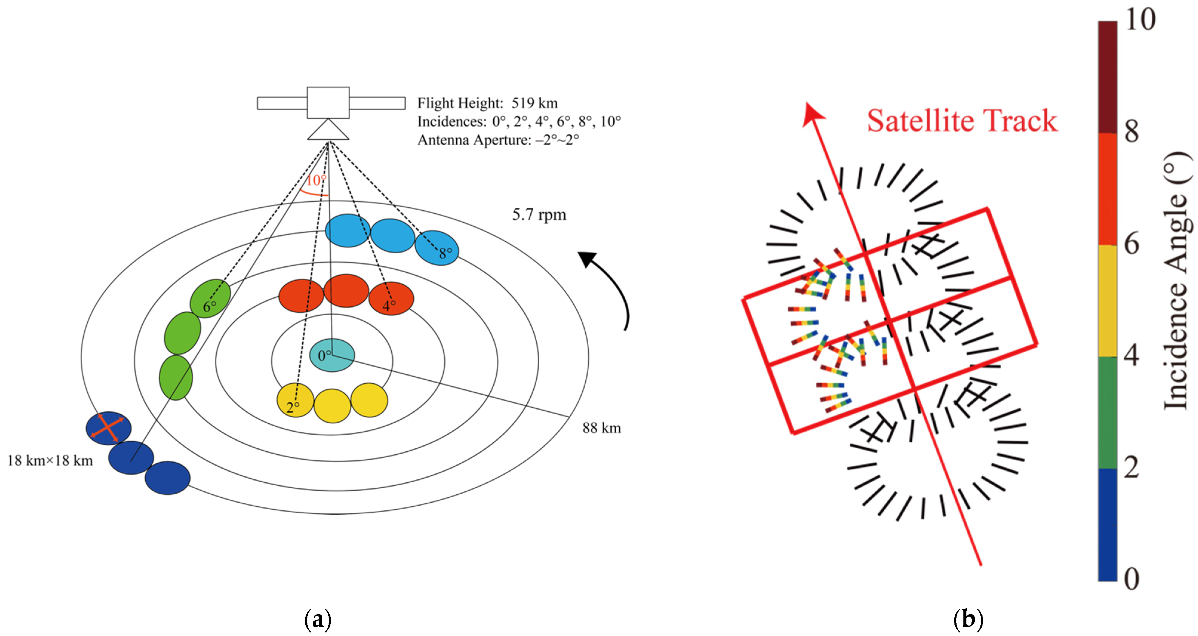
2.1. SWIM Data Onboard CFOSAT

In this study, we collected the CFOSAT data from January 2020 to December 2022. Significant wave heights from the SWIM were compared with simulations from the SWAN model in the East Pacific Ocean, and the SWIM-measured wave spectra were validated against the SAR-derived wave spectra from GF-3 SAR images located in China seas. These data were processed to be Level-2 (L-2) products, mainly including winds measured by the RFSCAT and waves from the SWIM instrument, which have been released since July 2019. Figure 1a illustrates the principal SWIM at incidence angles from 0° to 10°, showing that the CFOSAT footprint has a spatial coverage of 18 × 18 km in a spiral direction of 360°. The SWIM-measured wave spectrum was provided at incidence angles of 6°, 8° and 10° following each footprint in order to obtain reliable wave data. The top view of the SWIM imaging mode is illustrated in Figure 1b, in which the radar beams at six incidence angles are scanning the sea at the same time. It is important to note that the products derived from SWIM are the average values of two boxes at the left side or right side.

2.2. Model Settings of SWAN and NDBC Buoys

Because SWIM data rarely match up with moored buoys and altimeters, the third-generation SWAN numerical wave model (version 4.12) developed by the Delft University of Technology was used to simulate the sea surface wave fields in coastal waters [40]. As referred to in the conclusion of Stopa and Cheung (2014) [41], European Centre for Medium-Range Weather Forecasts (ECMWF) reanalysis interim winds are reliable at a regular sea state, based on 30 years of data collection. The forcing winds employed the global gridded atmospheric marine reanalysis data with a spatial resolution of 0.25° grid and an interval of 1 h, which were provided by the ECMWF reanalysis system (ERA-5). Topography data were provided by the General Bathymetric Chart of the Oceans (GEBCO) from the British Oceanographic Data Centre (BODC). The simulation regions were selected from longitude 165°W to 79°W and latitude 9°N to 44°N in the East Pacific Ocean. The SWAN simulation required the following switch settings:

• The two-dimensional wave spectrum was resolved into 24 regular azimuthal directions with a 15° step;
• The frequency bins ranged logarithmically from 0 to 1, at an interval of Δf/f = 0.903;
• The spatial resolution of the simulated wave fields was a 0.1° grid with a 60 min temporal resolution;
• The input/dissipation terms were selected, referred to as nonlinear saturation-based white-capping combined with wind input (WESTH);
• The various physical processes included white-capping (WCAPping), nonlinear quadruplet wave interactions (QUADrupl), depth-induced wave breaking in shallow waters (BREaking), bottom friction (FRICtion) and triad wave–wave interactions (TRIad).

As an example, the map of significant wave height from the SWAN model on 25 August 2020 at 18:00 UTC is presented in Figure 2, in which the colored footprints represent the SWIM-measured significant wave heights at the nadir incidence angle. It is clear that the SWAN-simulated significant wave height pattern is roughly consistent with the SWIM-measured significant wave heights. We think the deviation at the coastal water is probably caused by the time difference between them and complicate oceanic dynamics, i.e., tide, front and eddy.

At present, the NDBC buoys from NOAA are available for any investigators performing scientific research [42]. In order to validate the SWAN-simulated results, we also collected the wave measurements from NDBC buoys in the East Pacific Ocean. The geographic locations of the NDBC buoys in the East Pacific Ocean overlaid by the water depth are depicted as the black rectangles in Figure 3. The following metric parameters are used to evaluate the error of the SWAN-simulated wave:

$$\mathrm{Bias} = \frac{1}{n}{{\displaystyle \sum }}_{i=1}^n(X_i-Y_i),$$

(1)

$$\mathrm{RMSE} = \sqrt{\frac{1}{n}{{\displaystyle \sum }}_{i=1}^n{\left(X_i-Y_i\right)}^2 },$$

(2)

in which X_i and Y_i represents the significant wave height values of two sources. The comparison of more than 2000 matchups between SWAN-simulated significant wave heights and measurements from NDBC buoys on June–September 2020 is presented in Figure 4, revealing a 0.42 m RMSE in the significant wave height and −0.09 bias. In this sense, it is believed that the SWAN-simulated waves are reliable for this study.

2.3. GF-3 Images

Since August 2016, the GF-3 satellite has operationally released SAR images to the China Center for Resource Satellite Data and Applications (CRESDA) and the National Ocean Satellite Application Center (NSOAS). GF-3 SAR has 12 imaging modes, e.g., spotlight (SL), fine strip (FS), quad-polarization strip (QPS) and wave mode (WAV). In this study, the footprints of CFOSAT passed more than 300 GF-3 SAR images, which were acquired in QPS mode. These VV-polarization images were taken in China seas and have a pixel size of 10 m in both the azimuth and range directions, with a 100 km swath coverage. Note that the time difference between the GF-3 SAR images and the CFOSAT data was < 1 h. Figure 5a shows a calibrated GF-3 image acquired on 15 February 2022 at 21:51 UTC. The red circles present the geographic locations from the SWIM wave product with a spatial coverage of about 18 × 18 km, which were used for analyzing the wave spectra between GF-3 and CFOSAT. The two-dimensional wave spectrum from SWIM at an incidence angle of 10° corresponding to the red circle is presented in Figure 5b. It is observed that the true wave direction is difficult to obtain due to the 180° ambiguity of the SWIM-measured wave spectrum.

3. Methodology

The PFSM algorithm is a theoretically based method used to retrieve waves from SAR images based on the SAR wave mapping mechanism. In particular, the key to the PFSM algorithm is that an SAR intensity spectrum is decomposed into a nonlinearly mapped portion induced by the wind–sea interactions and a linear portion induced by wind-induced waves at relative long wavelength and swells. The separation wave number k_s calculated by Equation (3) was used to obtain the 2 corresponding portions from an SAR-measured spectrum:

$$k_s={\left[\frac{2.87g{V}^2}{R^2{U}_{10}^4{\cos }^2\phi \left({\sin }^2{\phi \sin }^2{\theta +\cos }^2\mathsf{\phi }\right)}\right]}^{0.33},$$

(3)

where g is the gravitational acceleration of 9.8 m/s²; V is the satellite flight velocity, assumed to be 7600 m/s for the GF-3 SAR; R is the satellite slant range in m; U₁₀ is the SAR-derived sea surface wind speed at a height of 10 m in m/s; θ is the radar incidence angle in degrees; and φ is the angle of the wave propagation direction relative to the radar look direction in degrees. It should be noted that U₁₀ was retrieved using the geophysical model function (GMF) CSARMOD-GF specially designed for re-calibrated images [43], which describes an empirical relationship between a wind vector and a co-polarized SAR backscattering signal expressed as a normalized radar cross-section united in linear ${\sigma }_0$:

$${\sigma }_0{=B}_0{(1+B}_1{\cos \Psi +B}_2\cos 2\Psi ),$$

(4)

in which matrix B consists of the U₁₀ and θ functions, and $\Psi$ is the angle of the wave propagation direction relative to the radar look direction. In this study, we directly applied the prior information to the wave propagation direction.

The portion of the SAR spectrum at wave numbers < k_s represents the linear mapping component induced by wind-induced waves at relative long wavelength and swells; in contrast, the left portion at wave numbers > k_s is mapped by the non-linear wind–sea mapping component. The wave numbers in the GF-3 spectrum here range from 0.0015 rad/s to 0.1058 rad/s. As for wind–sea retrieval in the PFSM algorithm, a best-fit “first-guess” wave spectrum was constructed using the well-known JONSWAP parametric model [44], utilizing the SAR-derived U₁₀ when searching for the 2 best-fit parameters, e.g., wave speed at peak c_p and wave propagation direction at peak ϕ. This method requires 3 steps: (1) the c_p and ϕ are directly obtained from the SAR intensity spectrum and treated as the first-guess values; (2) the value of c_p is searched in the range of 0.4 to 1.6 times the first-guess value at an interval of 0.2 m/s, and the value of ϕ is searched in the range of 0.8 to 1.2 at an interval of 2°; and (3) the SPRA scheme is employed in order to determine the best-fit values of the c_p and ϕ using a minimization procedure. The wind–sea spectrum is continuously inverted by minimizing a cost function J, similar to the MPI scheme. Simultaneously, the swell spectrum is linearly obtained by solving the SAR intensity spectrum at wave numbers smaller than k_s without considering the velocity bunching; that is, the tilt and hydrodynamic modulations are only included in the inversion scheme. Ultimately, the wave spectrum is composed of two retrieval portions.

$$J =\int {\left[I_k-{\overline{I}}_k\right]}^{2}dk+\mu \int {\left\{\frac{\left[E_k-{\overline{E}}_k\right]}{\left[B+{\overline{E}}_k\right]}\right\}}^{2}dk,$$

(5)

in which Ī_k is the first-guess wind–sea spectrum in term of k, I_k is the retrieved two-dimensional wave spectrum, Ē_k is the simulated SAR spectrum, E_k is the SAR spectrum, μ is the weight coefficient and the small positive number B is assumed to be 0.001 to ensure the inversion convergence. At present, algorithm PFSM has been implemented for GF-3 [45] and TerraSAR-X wave retrieval [46].

Using Equation (6), the significant wave height H_s is calculated from an inverted one-dimensional wave spectrum S_k at wave number k:

$$H_s=4 \times \sqrt{\int S_{k}dk},$$

(6)

The RMSE and bias exhibited in Equations (1) and (2) are used for the analyzing the metric error of wave parameters, e.g., significant wave height, peak wave length and peak wave period. In addition, two variables, the correlation coefficient (Cor) and the squared error (Err), are employed to describe the similarity of wave spectrum.

$$Cor=\frac{\int P_k{Q}_{k}dk}{\sqrt{\int P_k^{2}dk\int Q_k^{2}dk}},$$

(7)

$$Err =\frac{\int {\left[P_k-Q_k\right]}^{2}dk}{ \sqrt{\int P_k^{2}dk\int Q_k^{2}dk}}$$

(8)

in which P_k and Q_k represent the SWIM-derived wave spectrum and referred spectrum from SAR or SWAN. Note that the wave spectra of two sources are close as Cor approaches 1 and becomes smaller than that of Err.

4. Results

In this section, we present the comparisons between SWIM measurements and hindcasting waves by SWAN and the retrievals from GF-3 images. At last, the error analysis considering the background dynamics, i.e., wind, wave, current and sea level, is conducted.

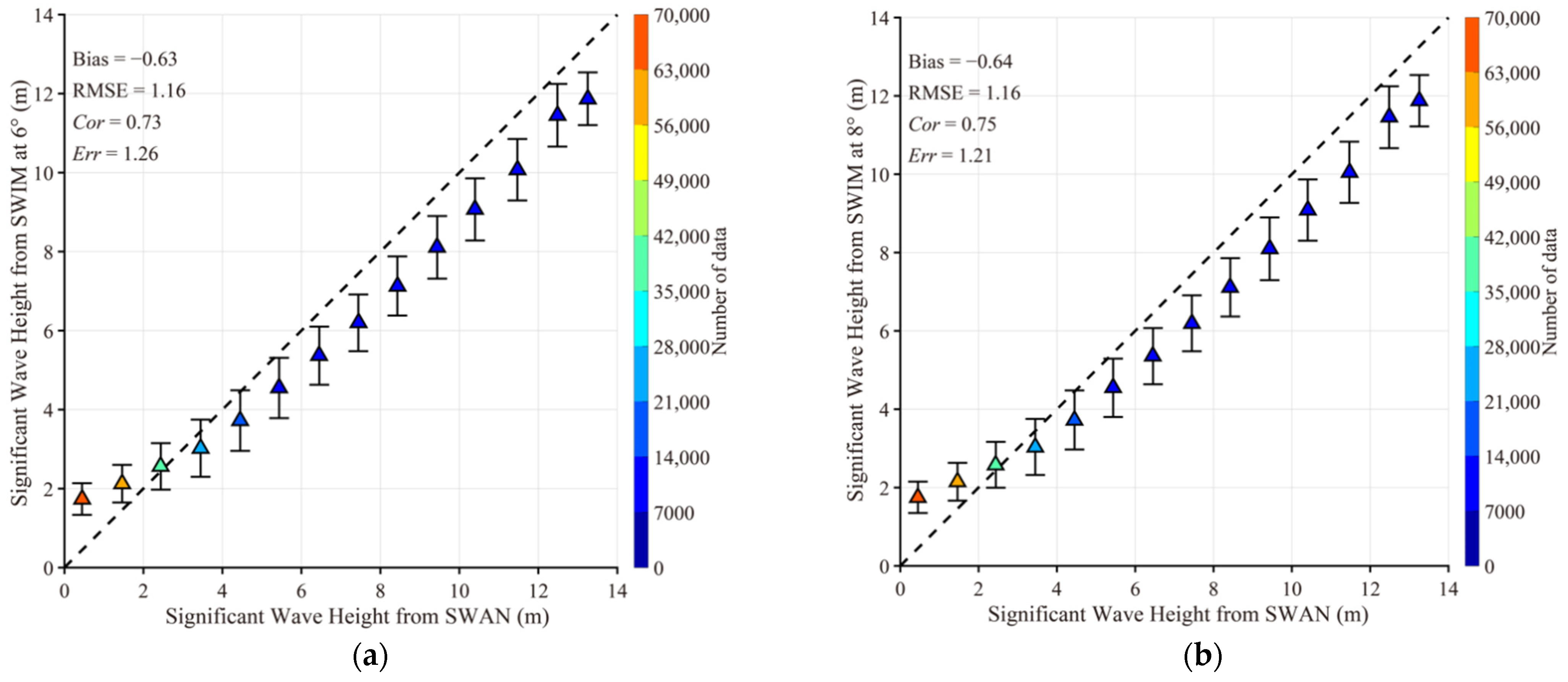
4.1. Comparison between SWIM Waves with SWAN-Simulated Results

Figure 6 provides a visual comparison of the SWIM-measured significant wave heights and the SWAN-simulated results at incidence angles of 6° (Figure 6a), 8° (Figure 6b), 10° (Figure 6c) and the average of the three incidence angles (Figure 6d). The comparison of significant wave height was processed at a 0.5 m bin up to 14 m. It was discovered that the analysis at an incidence angle of 10° performed well, as indicated by a 1.02 m RMSE with a 0.79 Cor and 1.17 Err, which exceeded the results at other incidence angles. Moreover, the SWIM-measured significant wave heights were overestimated at a particular sea state and then underestimated with an increasing significant wave height. Similarly, the comparisons of peak wave length and peak wave period were processed at a 20 m bin and 1 s bin, respectively. It is also found in Figure 7e,f that the SWIM products at an incidence angle of 10° have a better performance, e.g., a 35.52 m RMSE for peak wave length and a 0.82 s RMSE for peak wave period, which are lower than the statistical results at incidence angles of 6° (Figure 7a,b) and 8° (Figure 7c,d). However, there is likely to be a systematic negative difference between SWIM and SWAN values through the combination at incidence angles of 6°, 8° and 10°, e.g., a bias of ~−0.5 m at a significant wave height greater than 3 m (Figure 6d), bias of ~−30 m at a peak wave length greater than 220 m (Figure 7g) and bias of ~−1.0 s at a peak wave period greater than 12 s (Figure 7h). The parameter, called the frequency width, relates with the shape of the wave spectrum. The finding in [47] concludes that the SWIM directional spread at the peak is the smallest for swell. In this sense, we think that the difference between SWIM and SWAN values at a high sea state could be caused by a narrow frequency distribution of the SWIM spectrum at swell and mature conditions.

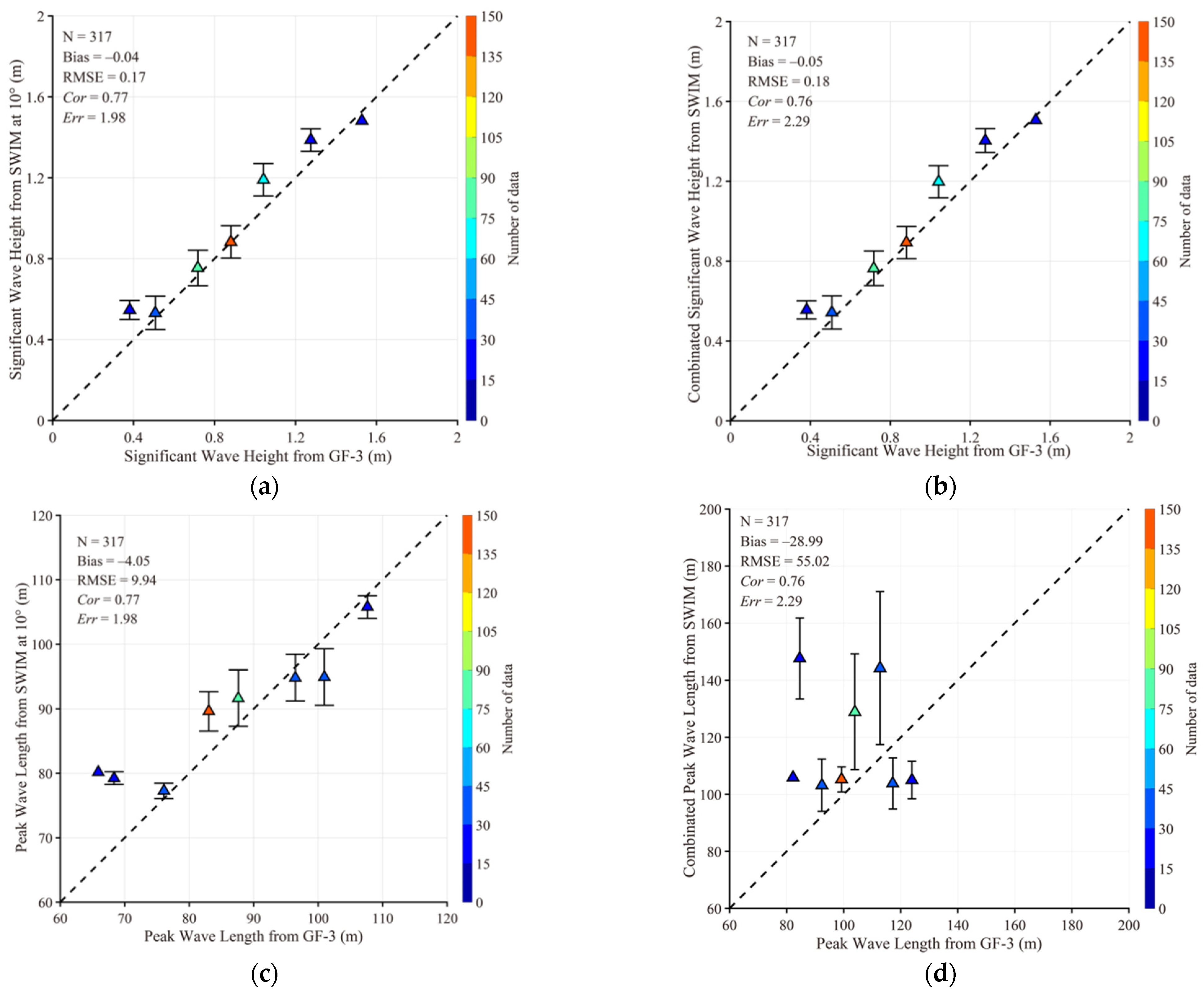
4.2. Comparison between SWIM Waves with GF-3 Retrievals

Here, the performance of SWIM wave spectra derived at three incidence angles is investigated. We analyzed more than 500 GF-3 SAR images covering the CFOSAT footprints, in which the time difference was <1 h. The sub-scenes extracted from the GF-3 SAR images in Figure 5 using a 1024 × 1024 pixel box (a spatial coverage of ~10 km), in which wave streaks were apparently observed, are presented in Figure 8a. Specifically, the inhomogeneous sub-scenes are excluded due to the poor quality of the sub-scenes, where the ratio of the image variance and squared image mean is greater than 1.05 [48]. Figure 8b shows the two-dimensional SAR spectra of the extracted sub-scenes, where the corresponding point coordinates are [27.2750°N, 122.4122°E], which is the closest point between the GF-3 sub image and the red point in Figure 5a, in which it can be seen that the structures of the SAR spectra are symmetrical. The PFSM algorithm was then applied to these sub-scenes in order to retrieve the wave spectra for the above cases.

The GF-3 SAR-derived wave spectra were compared with the SWIM-measured wave spectra, as shown in Figure 9. It was found that the general energy of the SWIM-measured wave spectra, which is calculated by the total area covered by the colored curves relative to the wave number and is represented by significant wave height, decreased with an increasing incidence angle. Moreover, in terms of the approximate spectrum shape and dominant wave propagation velocity, the GF-3 SAR-derived wave spectra were most consistent with the SWIM-measured wave spectra at an incidence angle of 10°. Due to velocity bunching, the short waves with wave numbers > 0.1 rad/m (i.e., wavelengths < 60 m) were undetectable in the SAR-derived wave spectra, indicating an apparent cutoff at such conditions. The wavelengths of the SWIM-measured wave spectra, however, were up to 30 m, with an about 0.2 rad/m wave number. Significant wave height represents the integral over frequencies and directions of the two-dimensional wave spectrum from the model or the specific sensor with a high-frequency cutoff; however, the cutoff wave numbers are different for SAR and SWIM.

Figure 10 shows the comparisons from all available matchups (>300 samples) at a regular sea state (significant wave heights < 2 m) between SWIM products at two incidence angles of 6° and 8° and retrievals from GF-3 SAR in 2020–2022, i.e., significant wave heights (Figure 10a,b), peak wave length (Figure 11c,d) and peak wave period (Figure 10e,f). Figure 11 shows the comparisons between SWIM products at an incidence angle of 10° and retrievals from GF-3 SAR. It is observed that the statistical results (i.e., a 0.77 Cor and 1.98 Err for the wave spectrum, 0.17 m RMSE for significant wave height, 9.94 m RMSE in peak wave length and 0.44 s RMSE in peak wave period) at an incidence angle of 10° (Figure 11a–c) are better than those (i.e., a 0.76 Cor and a 0.29 Err for wave spectrum, a 0.18 m RMSE in significant wave height, a 78.11 m RMSE in peak wave length and a 1.90 s RMSE in peak wave period) achieved from the combination at three incidence angles of 6°, 8° and 10° (Figure 11d–f). There seem to be large errors in peak wave period and peak wave length calculated from SWIM-measured wave spectra at two incidence angles of 6° and 8°. The different cutoff wavelength of the SWIM wave is smaller than that on GF-3, as exhibited in Figure 9, leading to the dominant wave energy of the SAR-derived wave spectrum mostly shifting toward a low frequency. This behavior is anticipated to be further studied through more GF-3 images collocated with SWIM measurements. Collectively, we believe that the SWIM wave data are a valuable source, especially for global wave analysis, although a 180° ambiguity in the wave direction needs to be resolved for SWIM observations. However, this work is a study that compares the GF-3 SAR-derived and SWIM-measured wave spectra, and a more collocated dataset needs to be collected for further validation at an extreme sea state, especially in tropical cyclones.

4.3. Discussions

As a matter of fact, the dynamics have an influence on the uncertainties of the SWIM product. Here, the difference in significant wave height between SWIM at an incidence angle of 10° and SWAN with respect to SWIM-measured wind speed, simulated significant wave height from SWAN and sea surface current and sea level from the 0.08° gridded Hybrid Coordinate Ocean Model (HYCOM) dataset at intervals of 3 h is investigated between January and July 2020, as exhibited in Figure 12. It is observed that the bias (SWIM minus SWAN) grows at a wind speed ranging from 0 to 5 m/s and that this behavior is also found at a wind speed greater than 10 m/s. With the growth in sea state (i.e., significant wave height > 4 m), the bias remains at −0.6 between the simulated significant wave height from SWAN and SWIM, indicating that the SWIM product can still be used for research on extreme waves. However, the bias has no significant correlation with current and sea level. It is reasonable that the wave is mainly determined by wind stress [49].

5. Conclusions

At present, wave monitoring is a topic of interest in the ocean remote sensing community. Since August 2019, CFOSAT has been successfully functioning and has operationally released wind and wave data from the CNES and CNSA. The SWIM instrument on board the CFOSAT is an advanced RAR technology designed to detect wave spectra over global seas, and follows the satellite orbit and has five off-nadir footprints of 18 × 18 km. Meanwhile, the Chinese GF-3 and its successor SAR also provide valuable information on related marine and atmospheric science applications [50]. The main purpose of our work was to make a preliminary attempt to analyze the wave parameters calculated from the wave spectrum measured by SWIM, which were compared with GF-3 SAR and SWAN simulations. This result is not only an evaluation of the SWIM spectral data, but also an important reference for oceanography research utilizing the SWIM spectral data.

Sea surface wind and wave data from SWIM available for this study were collected during the mission period from January 2020 to December 2022. The third-generation numeric model, denoted as SWAN, was employed to simulate waves in the Eastern Pacific Ocean and the China seas. Significant wave heights simulated by SWAN were validated against the measurements from NDBC buoys, yielding that the RMSE is 0.42 m and the bias is −0.09 m; therefore, the SWAN-simulated results were reliable for this study. The statistical analysis revealed that the RMSE in the SWIM-measured and SWAN-simulated significant wave heights at an incidence angle of 10° was 1.02 m with a 0.79 Cor and 1.17 Err up to 14 m, while the RMSEs were >1.1 m with Cors < 0.76 and Errs > 1.2 at the other incidence angles. Also, other SWIM-measured wave parameters at an incidence angle of 10° are reliable, e.g., a 35.52 m RMSE for peak wave length and a 0.82 s RMSE for peak wave period. We also extracted the wave spectra from a few sub-scenes of more than 300 GF-3 SAR images using the PFSM algorithm. We found that the general energy of the SWIM-measured wave spectra decreased with an increasing incidence angle, and the results of the 10° incidence angle were closest to the GF-3 SAR-derived wave spectra. The advantage of the SWIM-measured waves is that short waves, i.e., wavelengths < 60 m in our study, are detectable, which benefits the discovery of small-scale air–sea interactions. Available matchups (>300 samples) between SWIM at an incidence angle of 10° and GF-3 retrievals indicate a 0.17 m RMSE in significant wave heights with a 0.77 Cor and 1.98 Err, a 9.94 m RMSE in peak wave length and a 0.44 s RMSE in peak wave period, which is better than those achieved at other incidence angles. In addition, there are large errors in the peak wave period and peak wave length calculated from SWIM-measured wave spectra at two incidence angles of 6° and 8°, which are probably caused by the different cutoff wavelength between SWIM and GF-3. The statistical analysis of significant wave height between SWIM at an incidence angle of 10° and SWAN shows that bias (SWIM minus SWAN) remains at −0.6 at significant wave heights greater than 4 m, indicating the applicability of the SWIM product at an extreme sea state. Collectively, it is concluded that the SWIM-measured wave spectrum at an incidence angle of 10° is recommended for use in the oceanography research.

In the future, more data are expected that can be used to study the accuracy of SWIM-measured products, especially their performance at an extreme sea state, i.e., tropical cyclones and the Arctic Ocean [51]. In particular, the influence of precipitation and wave breaking on the SWIM products is anticipated to be studied. Additionally, we will promote this research campaign and attempt to evaluate the applicability of wave observations using CFOSAT, GF-3 SAR [52] and HY-2B in typhoons crossing the Western Pacific Ocean, which could prompt the development of typhoon dynamics research.

References

1. Liu, Q.X.; Alexander, V.B.; Stefan, Z.; Young, L.R.; Guan, C.L. Wind and wave climate in the Arctic Ocean as observed by Altimeters. J. Climate 2016, 29, 7957–7975. [Google Scholar] [CrossRef]
2. Gao, Y.; Guan, C.L.; Sun, J.; Xie, L. Tropical cyclone wind speed retrieval from dual-polarization Sentinel-1 EW mode products. J. Atmos. Ocean. Technol. 2020, 3, 1713–1724. [Google Scholar] [CrossRef]
3. Hauser, D.; Tison, C.; Amiot, T.; Delaye, L.; Corcoral, N.; Castillan, P. SWIM: The first spaceborne wave scatterometer. IEEE Trans. Geosci. Remote Sens. 2017, 55, 3000–3014. [Google Scholar] [CrossRef]
4. Shao, W.Z.; Jiang, T.; Zhang, Y.; Shi, J.; Wang, W. Cyclonic wave simulations based on WAVEWATCH-III using a sea surface drag coefficient derived from CFOSAT SWIM data. Atmosphere 2021, 12, 1610. [Google Scholar] [CrossRef]
5. Zhu, J.T.; Dong, X.L.; Lin, W.M.; Zhu, D. A preliminary study of the calibration for the rotating fan-beam scatterometer on CFOSAT. IEEE J. Sel. Topics Appl. Earth Observ. Remote Sens. 2015, 8, 460–470. [Google Scholar] [CrossRef]
6. Wang, L.L.; Ding, Z.Y.; Zhang, L.; Yan, C. CFOSAT-1 realizes first joint observation of sea wind and waves. Chin. J. Aeronaut. 2019, 20, 22–29. [Google Scholar]
7. Wang, J.K.; Aouf, L.; Dalphinet, A.; Zhang, Y.G.; Xu, Y.; Hauser, D.; Liu, J.Q. The wide swath significant wave height: An innovative reconstruction of significant wave heights from CFOSAT SWIM and scatterometer using deep learning. Geophys. Res. Lett. 2021, 48, e2020GL091276. [Google Scholar] [CrossRef]
8. Xu, Y.; Liu, J.Q.; Xie, L.L.; Sun, C.R.; Liu, J.P.; Li, J.Y. China-France Oceanography Satellite (CFOSAT) simultaneously observes the typhoon-induced wind and wave fields. Acta Oceanol. Sin. 2019, 38, 158–161. [Google Scholar] [CrossRef]
9. Grigorieva, V.G.; Badulin, S.I.; Gulev, S.K. Global validation of SWIM/CFOSAT wind waves against voluntary observing ship data. Earth Space Sci. 2022, 9, e2021EA002008. [Google Scholar] [CrossRef]
10. Lin, C.C.; Rommen, B.; Wilson, J.; Impagnatiello, F.; Park, P.S. An analysis of a rotating, range-gated, fanbeam spaceborne scatterometer concept. IEEE Trans. Geosci. Remote Sens. 2000, 38, 2114–2121. [Google Scholar]
11. Liu, J.Q.; Lin, W.M.; Dong, X.L.; Lang, S.Y.; Yun, R.S.; Zhu, D.; Zhang, K.; Sun, C.R.; Mu, B.; Ma, J.Y.; et al. First results from the rotating fan beam scatterometer onboard CFOSAT. IEEE Trans. Geosci. Remote Sens. 2020, 58, 8793–8806. [Google Scholar] [CrossRef]
12. Ebuchi, N. Evaluation of NSCAT-2 wind vectors by using statistical distributions of wind speeds and directions. J. Oceanogr. 2000, 56, 161–172. [Google Scholar] [CrossRef]
13. Tsai, W.; Graf, J.E.; Winn, C.; Huddleston, J.N.; Dunbar, S.; Freilich, M.H.; Wentz, F.J.; Long, D.G.; Jones, W.L. Postlaunch sensor verification and calibration of the NASA scatterometer. IEEE Trans. Geosci. Remote Sens. 1999, 37, 1517–1542. [Google Scholar] [CrossRef]
14. Figa-Saldana, J.; Wilson, J.J.; Attema, E.; Gelsthorpe, R.; Drinkwater, M.R.; Stoffelen, A. The advanced scatterometer (ASCAT) on the meteorological operational (MetOp) platform: A follow on for European wind scatterometers. Can. J. Remote Sens. 2002, 28, 404–412. [Google Scholar] [CrossRef]
15. Spencer, M.W.; Wu, C.; Long, D.G. Improved resolution backscatter measurements with the SeaWinds pencil-beam scatterometer. IEEE Trans. Geosci. Remote Sens. 2000, 38, 89–104. [Google Scholar] [CrossRef]
16. Shao, W.Z.; Jiang, T.; Jiang, X.W.; Zhang, Y.G.; Zhou, W. Evaluation of sea surface winds and waves retrieved from the Chinese HY-2B data. IEEE J. Sel. Topics Appl. Earth Observ. Remote Sens. 2021, 14, 9624–9635. [Google Scholar] [CrossRef]
17. He, J.N.; Guo, W.; Zhu, D.; Zhao, F. Analysis on calibration for flight experiments of CFOSAT scatterometer by return signal simulator. Remote Sens. Technol. App. 2015, 30, 731–736. [Google Scholar]
18. Dong, X.L.; Zhu, D.; Lin, W.M.; Liu, H.G.; Jiang, J.S. Status and recent progresses of development of the scatterometer of CFOSAT. In Proceedings of the 2011 IEEE International Geoscience and Remote Sensing Symposium, Vancouver, BC, Canada, 24–29 July 2011; pp. 961–964. [Google Scholar]
19. Alpers, R.; Bruening, C. On the relative importance of motion-related contributions to the SAR Imaging mechanism of ocean surface waves. IEEE Trans. Geosci. Remote Sens. 1986, GE-24, 873–885. [Google Scholar] [CrossRef]
20. Ning, J.; Sun, L.N.; Cui, H.J.; Lu, K.X.; Wang, J. Study on characteristics of internal solitary waves in the Malacca Strait based on Sentinel-1 and GF-3 satellite SAR data. Acta Oceanol. Sin. 2020, 39, 151–156. [Google Scholar] [CrossRef]
21. Alpers, R.; Ross, B.; Rufenach, L. On the detectability of ocean surface waves by real and synthetic aperture radar. J. Geophys. Res. Ocean. 1981, 86, 6481. [Google Scholar] [CrossRef]
22. Hasselmann, K.; Hasselmann, S. On the nonlinear mapping of an ocean wave spectrum into a synthetic aperture radar image spectrum and its inversion. J. Geophys. Res. Ocean. 1991, 96, 10713. [Google Scholar] [CrossRef]
23. Mastenbroek, C.; Valk, C. A semiparametric algorithm to retrieve ocean wave spectra from synthetic aperture radar. J. Geophys. Res. Ocean. 2000, 105, 3497–3516. [Google Scholar] [CrossRef]
24. Schulz-Stellenfleth, J.; Lehner, S.; Hoja, D. A parametric scheme for the retrieval of two-dimensional ocean wave spectra from synthetic aperture radar look cross spectra. J. Geophys. Res. Ocean. 2005, 110, C05004. [Google Scholar] [CrossRef]
25. Sun, J.; Guan, C.L. Parameterized first-guess spectrum method for retrieving directional spectrum of swell-dominated waves and huge waves from SAR images. Chin. J. Oceanol. Limn. 2006, 24, 12–20. [Google Scholar]
26. Jiang, T.; Shao, W.Z.; Hu, Y.Y.; Zheng, G.; Shen, W. L-band analysis of the effects of oil slicks on sea wave characteristics. J. Ocean Univ. China 2023, 22, 9–20. [Google Scholar] [CrossRef]
27. Shao, W.Z.; Hu, Y.Y.; Jiang, X.W.; Zhang, Y.G. Wave retrieval from quad-polarized Chinese Gaofen-3 SAR image using an improved tilt modulation transfer function. Geo-Spat. Inf. Sci. 2023. [Google Scholar] [CrossRef]
28. Schulz-Stellenfleth, J.; Konig, T.; Lehner, S. An empirical approach for the retrieval of integral ocean wave parameters from synthetic aperture radar data. J. Geophys. Res. Ocean. 2007, 42, 10182–10190. [Google Scholar] [CrossRef]
29. Li, X.M.; Konig, T.; Schulz-Stellenfleth, J.; Lehner, S. Validation and intercomparison of ocean wave spectra inversion schemes using ASAR wave mode data. Int. J. Remote Sens. 2010, 31, 4969–4993. [Google Scholar] [CrossRef]
30. Stopa, E.; Mouche, A. Significant wave heights from Sentinel-1 SAR: Validation and applications. J. Geophys. Res. Oceans 2017, 122, 1827–1848. [Google Scholar] [CrossRef]
31. Pleskachevsky, A.; Jacobsen, S.; Tings, B.; Schwarz, E. Estimation of sea state from Sentinel-1 synthetic aperture radar imagery for maritime situation awareness. Int. J. Remote Sens. 2019, 40, 4104–4142. [Google Scholar] [CrossRef]
32. Sheng, Y.X.; Shao, W.Z.; Zhu, S.; Sun, J.; Yuan, X.Z.; Li, S.Q.; Shi, J.; Zuo, J.C. Validation of significant wave height retrieval from co-polarization Chinese Gaofen-3 SAR imagery using an improved algorithm. Acta Oceanol. Sin. 2018, 37, 1–10. [Google Scholar] [CrossRef]
33. Zhu, S.; Shao, W.Z.; Armando, M.; Shi, J.; Sun, J.; Yuan, X.Z.; Hu, J.C.; Yang, D.K.; Zuo, J.C. Evaluation of Chinese quad-polarization Gaofen-3 SAR wave mode data for significant wave height retrieval. Can. J. Remote Sens. 2019, 44, 588–600. [Google Scholar] [CrossRef]
34. Hao, M.Y.; Shao, W.Z.; Yao, R.; Zhang, Y.G.; Jiang, X.W. Improvement of quad-polarized velocity bunching modulation transfer function by C-band Gaofen-3 SAR. Remote Sens. Lett. 2023, 14, 968–978. [Google Scholar] [CrossRef]
35. Hauser, D.; Soussi, E.; Thouvenot, E.; Rey, L. SWIMSAT: A real-aperture radar to measure directional spectra of ocean waves from space–main characteristics and performance simulation. J. Atmos. Ocean. Technol. 2001, 18, 421–437. [Google Scholar] [CrossRef]
36. Hauser, D.; Tourain, C.; Hermozo, L.; Alraddawi, D.; Aouf, L.; Chapron, B.; Dalphinet, A.; Delaye, L.; Dalila, M.; Dormy, E.; et al. New observations from the SWIM radar on-board CFOSAT: Instrument validation and ocean wave measurement assessment. IEEE Trans. Geosci. Remote 2021, 59, 5–26. [Google Scholar] [CrossRef]
37. Ye, H.; Li, J.; Li, B.; Liu, J.; Tang, D.; Chen, W.; Yang, H.; Zhou, F.; Zhang, R.; Wang, S.; et al. Evaluation of CFOSAT scatterometer wind data in global oceans. Remote Sens. 2021, 13, 1926. [Google Scholar] [CrossRef]
38. Tang, S.L.; Chu, X.Q.; Jia, Y.J.; Li, J.M.; Liu, Y.T.; Chen, Q.; Li, B.; Liu, J.L.; Chen, W.Y. An appraisal of CFOSAT wave spectrometer products in the South China Sea. Earth Space Sci. 2022, 9, e2021EA002055. [Google Scholar] [CrossRef]
39. Zheng, K.W.; Osinowo, A.; Sun, J.; Hu, W. Long term characterization of sea conditions in the East China Sea using significant wave height and wind speed. J. Ocean. Univ. China 2018, 17, 733–743. [Google Scholar] [CrossRef]
40. Holthuijsen, L. The continued development of the third-generation shallow water wave model ‘SWAN’. Tu Delft Dep. Hydraul. Eng. 2001, 32, 185–186. [Google Scholar]
41. Stopa, J.E.; Cheung, K.F. Intercomparison of wind and wave data from the ECMWF Reanalysis Interim and the NCEP Climate Forecast System Reanalysis. Ocean Model. 2014, 75, 65–83. [Google Scholar] [CrossRef]
42. Teng, C.C. Ocean observation from NOAA national data buoy center’s platforms. In Proceedings of the SPIE—The International Society for Optical Engineering, Orlando, FL, USA, 5–9 April 2010; Volume 7678, pp. 13–17. [Google Scholar]
43. Shao, W.Z.; Nunziata, F.; Zhang, Y.G.; Corcione, V.; Migliaccio, M. Wind speed retrieval from the Gaofen-3 synthetic aperture radar for VV- and HH-polarization using a re-tuned algorithm. Eur. J. Remote Sens. 2021, 54, 318–337. [Google Scholar] [CrossRef]
44. Hasselmann, K.; Barnett, T.P.; Bouws, E.; Carlson, H.; Cartwright, D.E.; Enke, K.; Ewing, J.A.; Gienapp, H.; Hasselmann, D.E.; Kruseman, P.; et al. Measurements of Wind-Wave Growth and Swell Decay during the Joint North Sea Wave Project (JONSWAP); UDC 551.466.31; Deutches Hydrographisches Institut: Hamburg, Germany, 1973. [Google Scholar]
45. Shao, W.Z.; Jiang, X.W.; Sun, Z.F.; Hu, Y.Y.; Marino, A.; Zhang, Y.G. Evaluation of wave retrieval for Chinese Gaofen-3 synthetic aperture radar. Geo-Spat. Inf. Sci. 2022, 25, 229–243. [Google Scholar] [CrossRef]
46. Shao, W.Z.; Li, X.F.; Sun, J. Ocean wave parameters retrieval from TerraSAR-X images validated against buoy measurements and model results. Remote Sens. 2015, 7, 12815–12828. [Google Scholar] [CrossRef]
47. Merle, E.; Hauser, D.; Peureux, C.; Aouf, L.; Schippers, P.; Dufour, C.; Dalphinet, A. Directional and frequency spread of surface ocean waves from SWIM measurements. J. Geophys. Res. Oceans 2021, 126, e2021JC017220. [Google Scholar] [CrossRef]
48. Li, X.M.; Lehner, S.; Bruns, T. Ocean wave integral parameter measurements using Envisat ASAR wave mode data. IEEE Trans. Geosci. Remote Sens. 2011, 49, 155–174. [Google Scholar] [CrossRef]
49. Yao, R.; Shao, W.Z.; Hao, M.Y.; Zuo, J.C.; Hu, S. The Respondence of wave on sea surface temperature in the context of global change. Remote Sens. 2023, 15, 1948. [Google Scholar] [CrossRef]
50. Zhong, R.Z.; Shao, W.Z.; Zhao, C.; Jiang, X.W.; Zuo, J.C. Analysis of wave breaking on Gaofen-3 and TerraSAR-X SAR image and its effect on wave retrieval. Remote Sen. 2023, 15, 574. [Google Scholar] [CrossRef]
51. Liu, M.; Yan, R.; Zhang, J.; Xu, Y.; Chen, P.; Shi, L.; Wang, J.; Zhong, S.; Zhang, X. Arctic sea ice classification based on CFOSAT SWIM data at multiple small incidence angles. Remote Sens. 2022, 14, 91. [Google Scholar] [CrossRef]
52. Hu, Y.Y.; Shao, W.Z.; Jiang, X.W.; Zhou, W.; Zuo, J.C. Improvement of VV-polarization tilt MTF for Gaofen-3 SAR data of a tropical cyclone. Remote Sens. Lett. 2023, 14, 461–468. [Google Scholar] [CrossRef]
Figure 1. (a) Principal Surface Waves Investigation and Monitoring (SWIM) at incidence angles from 0° to 10° in a counterclockwise direction, in which the CFOSAT footprint has a spatial coverage of 18 × 18 km. (b) The top view following the satellite track, in which the products derived from SWIM are the average values of two boxes at the left side or right side.
Remotesensing 15 04402 g001
Figure 2. Map of significant wave heights from the Simulating Waves Nearshore (SWAN) model on 25 August 2020 at 18:00 UTC, in which the colored footprints represent the SWIM-measured significant wave heights at nadir incidence angle.
Remotesensing 15 04402 g002
Figure 3. Region from latitude 9°N to 44°N and longitude 70°W to 165°W used to simulate the wave fields by SWAN overlaying the water depth from the General Bathymetric Chart of the Oceans (GEBCO). The 2 black rectangles are the geographic locations of the National Data Buoy Center (NDBC) buoys selected for validating the simulations.
Remotesensing 15 04402 g003
Figure 4. Simulated significant wave heights from the SWAN model versus the co-located measurements from NDBC buoys from June to September 2020.
Remotesensing 15 04402 g004
Figure 5. (a) Calibrated GF-3 synthetic aperture radar (SAR) image acquired on 15 February 2022 at 21:51 UTC, in which the red circle is the geographic location of CFOSAT wave products at [27.29°N, 122.41°E]. (b) The two-dimensional wave spectrum from SWIM at incidence angle of 10° corresponding to the red circle.
Remotesensing 15 04402 g005
Figure 6. SWIM-measured significant wave height versus co-located measurements from the SWAN model for a 0.5 bin of significant wave height: (a) at incidence angle of 6°, (b) at incidence angle of 8°, (c) at incidence angle of 10° and (d) combination at incidence angles of 6°, 8° and 10°. The comparison of significant wave height was processed at a 0.5 m bin up to 14 m.
Remotesensing 15 04402 g006aRemotesensing 15 04402 g006b
Figure 7. SWIM-measured wave parameters, e.g., peak wave length and peak wave period, versus co-located measurements from the SWAN model: (a,b) at incidence angle of 6°; (c,d) at incidence angle of 8°; (e,f) at incidence angle of 10°; and (g,h) the combination at incidence angles of 6°, 8° and 10°. The comparisons of peak wave length and peak wave period were processed at a 20 m bin and 1 s bin, respectively.
Remotesensing 15 04402 g007aRemotesensing 15 04402 g007b
Figure 8. (a) Sub-scene corresponding to red point extracted from the GF-3 image acquired on 15 February 2022 at 21:51 UTC. (b) Two-dimensional SAR spectrum at the wave number corresponding to the sub-scene.
Remotesensing 15 04402 g008
Figure 9. Retrieval results for the one-dimensional SWIM-measured wave spectrum at various incidence angles and the GF-3 SAR-derived wave spectrum.
Remotesensing 15 04402 g009
Figure 10. SWIM-measured wave parameters versus co-located retrievals from the GF-3 images: (a) significant wave height at an incidence angle of 6° and (b) significant wave height at an incidence angle of 8°; (c) peak wave length at an incidence angle of 6° and (d) peak wave length at an incidence angle of 8°; (e) peak wave period at an incidence angle of 6° and (f) peak wave period at an incidence angle of 8°.
Remotesensing 15 04402 g010aRemotesensing 15 04402 g010b
Figure 11. SWIM-measured wave parameters at an incidence angle of 10° versus co-located retrievals from the GF-3 images: (a) significant wave height, (b) peak wave length and (c) peak wave period. SWIM-measured wave parameters from the combination at three incidence angles of 6°, 8° and 10° versus co-located retrievals from the GF-3 images: (d) significant wave height, (e) peak wave length and (f) peak wave period.
Remotesensing 15 04402 g011aRemotesensing 15 04402 g011b
Figure 12. Difference in significant wave height between SWIM at an incidence angle of 10° and SWAN with respect to (a) SWIM-measured wind speed, (b) simulated significant wave height from SWAN, (c) 0.08° gridded average sea surface current and (d) sea level from Hybrid Coordinate Ocean Model (HYCOM) dataset at intervals of 3-h.
Remotesensing 15 04402 g012aRemotesensing 15 04402 g012b
Disclaimer/Publisher’s Note: The statements, opinions and data contained in all publications are solely those of the individual author(s) and contributor(s) and not of MDPI and/or the editor(s). MDPI and/or the editor(s) disclaim responsibility for any injury to people or property resulting from any ideas, methods, instructions or products referred to in the content.