Article

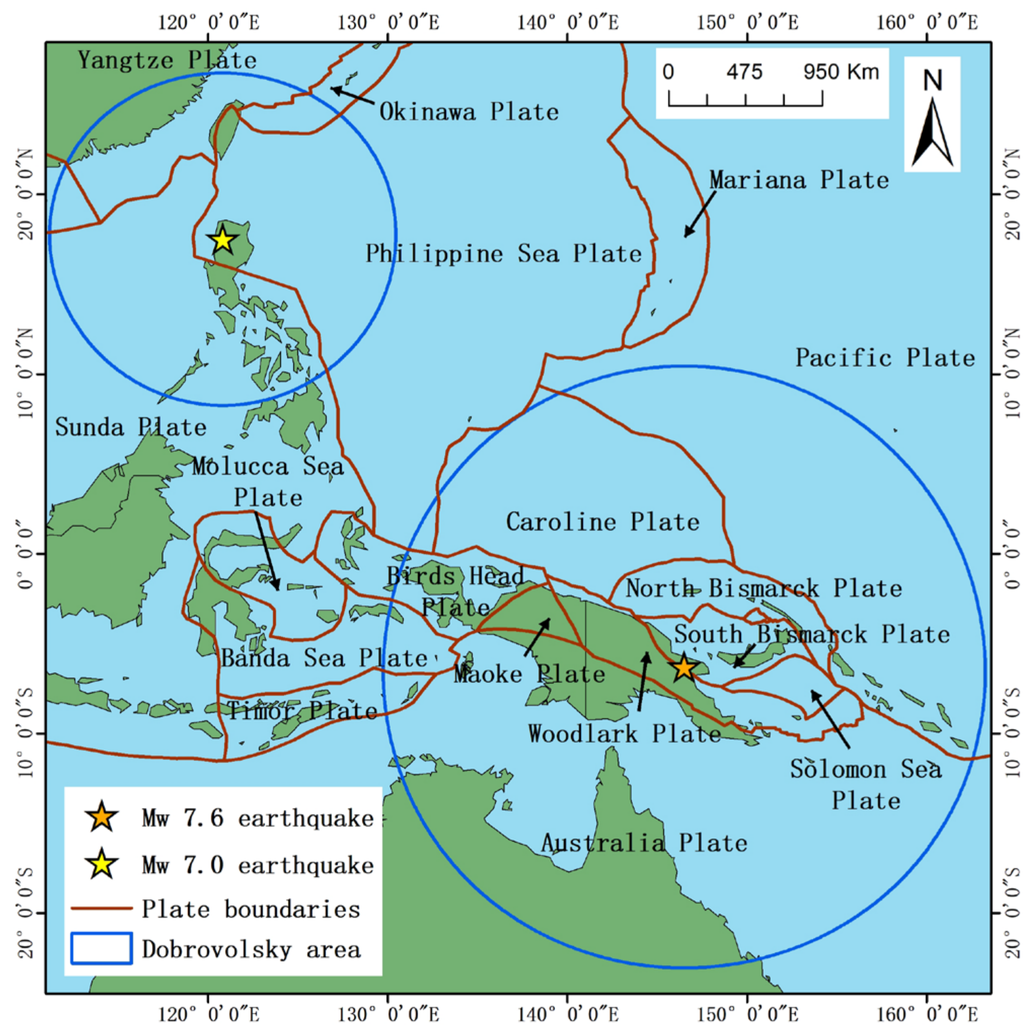
Analysis of Ocean–Lithosphere–Atmosphere–Ionosphere Coupling Related to Two Strong Earthquakes Occurring in June–September 2022 on the Sea Coast of Philippines and Papua New Guinea

1
College of Geo-Exploration Science and Technology, Jilin University, Changchun 130026, China
2
British Geological Survey, Keyworth, Nottingham NG12 5GG, UK
*
Author to whom correspondence should be addressed.
Remote Sens. 2023, 15(18), 4392; https://doi.org/10.3390/rs15184392
Submission received: 9 August 2023 / Revised: 30 August 2023 / Accepted: 5 September 2023 / Published: 6 September 2023

Abstract

:
Scientific progress in the context of seismic precursors reveals a systematic mechanism, namely lithosphere–atmosphere–ionosphere coupling (LAIC), to elaborate the underlying physical processes related to earthquake preparation phases. In this study, a comprehensive analysis was conducted for two earthquakes that occurred on the sea coast through tidal force fluctuation to investigate ocean–lithosphere–atmosphere–ionosphere coupling (OLAIC), based on oceanic parameters (i.e., sea potential temperature and seawater salinity), air temperature and electron density profiles. The interrupted enhancement and diffusion process of thermal anomalies indicate that the intensity of seismic anomalies in the atmosphere is affected by the extent of land near the epicenter. By observing the evolution of the ocean interior, we found that the deep water was lifted and formed upwelling, which then diffused along the direction of plate boundaries with an “intensification-peak-weakening” trend under the action of the accelerated subduction of tectonic plates. Furthermore, the analysis shows that the seismic anomalies have two propagation paths: (i) along active faults, with the surface temperature rising as the initial performance, then the air pressure gradient being generated, and finally the ionosphere being disturbed; (ii) along plate boundaries, upwelling, which is the initial manifestation, leading to changes in the parameters of the upper ocean. The results presented in this study can contribute to understanding the intrinsic characteristics of OLAIC.

1. Introduction

The issue of pronounced changes in different geospheres possibly correlated with seismic activity has been a consistent focal point for numerous researchers [1,2,3,4,5,6,7]. Many studies have furnished scientific evidence to elucidate diverse forms of pre-seismic and post-seismic comprehensive perturbations as manifestations of lithosphere–atmosphere–ionosphere coupling (LAIC) [8,9,10,11]. Until now, several theories have emerged to clarify the origin of seismic anomalies and the formation of coupling relationships [12,13,14,15], but this topic still requires further exploration. At present, few studies have correlated seismic anomalies in the ocean with LAIC. The evolution of seawater can facilitate a deeper comprehension of the transmission of subsurface anomalies and their association with higher-level anomalies. Therefore, it is expected that ocean–lithosphere–atmosphere–ionosphere coupling (OLAIC) will be developed for the enhancement of its theoretical basis.
A thermal anomalous signal is commonly regarded as the direct manifestation of earthquake precursor processes, and a variety of methods and data have found extensive utility in examining thermal anomalies linked to seismic events [3,16,17,18,19]. The elevated level of attention directed toward thermal anomalies is attributed to their association with tectonic movements and their potential to trigger other precursor phenomena [20]. To understand the temporal and spatial variation, as well as the transfer process of thermal anomalies, the tidal force fluctuation analysis (TFFA) was developed and then employed to identify atmospheric thermal anomalies linked to seismic activity [16,21,22,23,24]. This approach capitalizes on the distinctive traits of tidal force, that is, the indicator function in the seismic time domain [25]. Previously, TFFA was confined to detecting atmospheric anomalies, while the transmission of anomalies from the lithosphere to the ionosphere implies that tidal force fluctuations could potentially identify seismic anomalies across multiple layers and with a broader range of parameters [24]. Applying TFFA across the ocean, lithosphere, atmosphere and ionosphere could yield more significant observations.
Ionospheric perturbations have been highlighted as potential seismic precursors in numerous studies [2,8,9,10,26,27,28]. Researchers have focused on the different distributions of ionospheric anomaly, including temporal, horizontal and vertical spatial scales. Throughout earthquake preparation phases, the propagation of the resulting disturbance is a continuous process [10], and thus changes in the ionospheric vertical structure over time within a certain distance from the epicenter are indicative. Utilizing observations encompassing both land and sea areas proximate to the epicenter is essential. Applying the radio occultation technique, which can detect ionospheric structures around the world, the FORMOSAT-7/COSMIC-2 (F7/C2) mission provides sufficient soundings to compensate for the absence of terrestrial instruments extending over oceanic expanses.
Anomalies linked to earthquakes occurring on the sea coast have been previously documented to occasionally exhibit greater prominence [29,30] and have a temporal and spatial correlation with terrestrial and atmospheric anomalies [31,32]. The mobility of seawater and possible solid Earth–seafloor interactions related to earthquakes may lead to the wide diffusion and high intensity of seismic disturbances in the ocean. To verify the interactions, multi-parameter fluctuation on the sea surface needs to be explained by the evolution process of the ocean interior. Some studies have attributed seismic anomalies on the sea surface to the upwelling of cold water induced by tectonic activity [30,33,34]. However, the detection and analysis of seismic anomalies covering the large-scale horizontal and vertical space of ocean interior evolution are still vacant in the continuous time interval. In addition, some studies have undertaken the comparison of parameter fluctuations within the ocean near the occurrence of earthquakes with those observed in other geospheres. Comparative analysis reveals a discernible synchronicity between anomalies in sea surface temperature and land surface temperature [35]. Spatial-temporal analysis involving multiple parameters indicates a correlation between sea surface salinity concentration and atmospheric disturbances [36]. Evidence has also been provided by recent research regarding the potential link between seismicity-induced upwelling and surface atmospheric temperature [33]. Past studies have gradually established the embryonic framework of OLAIC. To further enhance the comprehensiveness of OLAIC, an investigation into the anomalous overall propagation process is imperative.
In the current work, we conducted a complementary analysis by integrating parameters of two earthquakes that occurred on the sea coast to understand the mechanisms of seismic anomalies in the ocean, lithosphere, atmosphere and ionosphere. In the pursuit of creating a comprehensive anomaly detection approach, the anomalies across multiple layers and their subsequent transmission processes were discerned using TFFA. The electron density (Ne) profiles covering land and sea from the F7/2C mission were used to report the vertical variation in the ionospheric structure resulting from earthquakes. The possible solid Earth–seafloor interactions related to earthquakes were analyzed using large-scale ocean interior evolution. This study aims to investigate OLAIC and to expose its manifestation and action mode on the spatiotemporal scale.

2. Materials and Methods

2.1. Seismic Data

As the largest island in the Philippine archipelago, Luzon is subjected to more pronounced fault activity owing to the relative movement between the Sunda plate and the Philippine Sea plate. In the southern sector of Luzon Island, the Philippine Sea Plate subducts westward beneath the Sunda Plate. In northern Luzon, particularly where the Mw = 7.0 earthquake occurred on 27 July 2022, the Sunda Plate subducts eastward beneath the Philippine Sea Plate. In contrast to the Mw = 7.0 earthquake, the plate motion in the vicinity of the Mw = 7.6 earthquake on 10 September 2022 was characterized by a greater degree of complexity. The earthquake was connected with the extensive converging movement of the Australia plate and the Pacific plate and with the interactions of other microplates, including the North Bismarck plate, the South Bismarck plate, the Solomon Sea plate and the Woodlark plate. The earthquakes studied here include the Mw = 7.0 and the Mw = 7.6 earthquakes, which arose from oblique reverse faulting and dipping fault mechanisms, respectively, and the location is shown in Figure 1.
Additionally, the coupling anomalies in multi-layers pertaining to the two earthquakes that occurred on the sea coast were examined. The earthquake data are sourced from the United States Geological Survey (https://earthquake.usgs.gov/earthquakes, accessed on 7 August 2023), as shown in Table 1.

2.2. Oceanic Data

In this study, sea potential temperature (SPT) and seawater salinity (SWS) are used to reflect anomalous changes in the ocean around the occurrence time of earthquakes. The oceanic data were acquired from Copernicus Marine Environmental Monitoring Service (CNEMS), which provides global ocean analysis and forecasts. We used daily updated data from the Global Ocean Physical Analysis and Forecasting Product (https://data.marine.copernicus.eu/products, accessed on 29 August 2023). Data with a horizontal resolution of 1/12° × 1/12° (approx. 8 km × 8 km) at 50 vertical levels (range from 0 to 5500 m with logarithmic space) assimilated temperature and salinity profiles. The mean error of SPT and SWS across 50 vertical levels, in comparison to on-site observations, scarcely surpassed 0.5 K and 0.01 PSU, respectively [37].

2.3. Air Temperature

The air temperature data were gathered from National Center for Environmental Prediction (NCEP) reanalysis data, which are collated by the National Center for Atmospheric Research (NCAR) and NCEP [38]. The reanalysis data with 1° × 1° horizontal resolution and 6 h temporal resolution included the ground surface and 26 isobaric levels [39]. We selected the ground surface and five isobaric levels. Specifically, the isobaric levels at 950 hPa, 925 hPa, 900 hPa, 850 hPa and 800 hPa were used to detect anomalies for the Mw = 7.0 earthquake, and the isobaric levels at 925 hPa, 900 hPa, 850 hPa, 800 hPa and 750 hPa were used to detect anomalies for the Mw = 7.6 earthquake.

2.4. Electron Density

As a low-orbit cluster of six low-Earth-orbit (LEO) satellites, F7/C2 was launched on 25 June 2019 with an inclination of 24° and the ability to provide over 4000 ionospheric soundings per day at low latitudes. The six LEO satellites, namely Flight Models 1 through 6 (FM1-FM6), collaboratively furnish holistic understanding regarding the vertical electron density profile encompassing the ionosphere. Each LEO satellite in this constellation is equipped with advanced GPS radio occultation receivers. The Ne profiles are retrieved by utilizing variations in a radio signal transmitted by the GNSS satellite while passing through the ionosphere.
Due to the intrinsic properties of the ionosphere, the diurnal and nocturnal Ne profiles exhibit significant disparities. The photochemical process dominates the characteristics of the ionosphere at E and F1 layers in the daytime, and thus Ne profiles drop dramatically to vanishing at night because of the high loss rate [40]. The loss rate in the F2 layer (mainly higher than 200 km altitude) and above decreases with rising altitude, which reduces the weakening amplitude of Ne profiles at night [41]. Typically, Ne profiles in the daytime are significantly enhanced overall compared to at night [40,42]. Therefore, in this study, we separated diurnal and nocturnal Ne. The time range from 15:00 UT to 23:00 UT was used to select nocturnal Ne profiles for the Mw = 7.0 earthquake, and the time range from 13:00 UT to 21:00 UT was used to select nocturnal Ne profiles for the Mw = 7.6 earthquake. Figure 2 shows the radio occultation soundings around two earthquakes on 22 August 2022 and 6 October 2022.

2.5. Tidal Force and Anomaly Detection

In our pursuit of understanding the transmission chain of seismic disturbances, we examined the amalgamation of processes through which anomalies traverse from the ocean to the ground surface, propagate through the atmosphere and subsequently influence the ionosphere. The ocean, atmosphere and ionosphere are subject to various disturbances, which produce a large number of subtle and messy fluctuations in each variable. Hence, there is a need to formulate a consistent method that can extract the abnormal evolution process with temporal and spatial rules. Tidal force plays an important role in this process, pushing the rocks to a state of criticality [43]. Researchers have established the basis for detecting thermal anomalies through tidal force variation [16,21,22,23,24]. Tidal Force Fluctuant Analysis (TFFA) is an approach used to identify thermal anomalies in the atmosphere. The method for computing tidal force potential has been detailed and described in references [16,21]. The initial TFFA is constrained by the requirement to establish the correlation between the timing of earthquakes and the tidal force potential. Given this problem, Xu et al. modified the TFFA method [24], which is the basis of anomaly detection through tidal force variation in this study.
We first applied the TFFA to detect atmospheric thermal anomalies. After calculating tidal force potential, the peak was taken as the first day of the next period, and the day before the next peak was taken as the last day of the period. The mean value of the whole period was set as the background at each pixel. The difference between the air temperature and the corresponding background value was used for the next analysis. The specific criteria [24] for detecting thermal anomalies related to earthquakes are as follows:
  • Thermal anomalies emerge from the bottom. As the altitude increases, thermal anomalies tend to diminish.
  • The distribution of thermal anomalies at each level coincides with the fault pattern.
  • Thermal anomalies spread on the time scale, and therefore thermal anomalies should last two consecutive days at least.
Similarly, we performed background value removal on SPT and SWS on the basis of TFFA. Within a tidal force period, the mean values of SPT and SWS for each pixel were established as background values. The corresponding difference between the original value and the background was obtained. From this foundation, daily variations in SPT anomalies and SWS anomalies were generated for the analysis of the upwelling formation.
Then, we conducted anomaly identification for Ne based on tidal force periods. The radio occultation soundings within ±5° latitude and longitude away from the epicenter were extracted, with a spatial range consistent with the study of air temperature, SPT and SWS. Note that such a study area was located within the Dobrovolsky radius [44] of both earthquakes. As described in Section 2.4, the daily data were divided into two groups, daytime and nighttime, due to significant differences in Ne profiles. The mean values of Ne profiles, separated by daytime and nighttime were calculated for each day, denoted as N e d a y and N e n i g h t , and N e d i f was obtained using N e d a y N e n i g h t . Based on the same tidal force periods as above, the mean profiles of each period were calculated as the background. The difference between N e d i f and background was defined as Δ Ne . The confidence bounds were computed through the mean value and interquartile range of Δ Ne , as shown in Equation (1).
U B = μ + 2 × I Q R L B = μ 2 × I Q R
where U B represents the upper bound, L B represents the lower bound, μ is the mean value of Δ Ne and I Q R is the interquartile range of Δ Ne .

3. Results

We examined various anomalies across multiple layers during six distinct periods of each earthquake, uncovering a spatiotemporal coupling phenomenon aligned with the propagation patterns of seismic anomalies. The investigated time spans for the two earthquakes that occurred on the sea coast encompassed 88 days and 89 days, as illustrated in Figure 3.

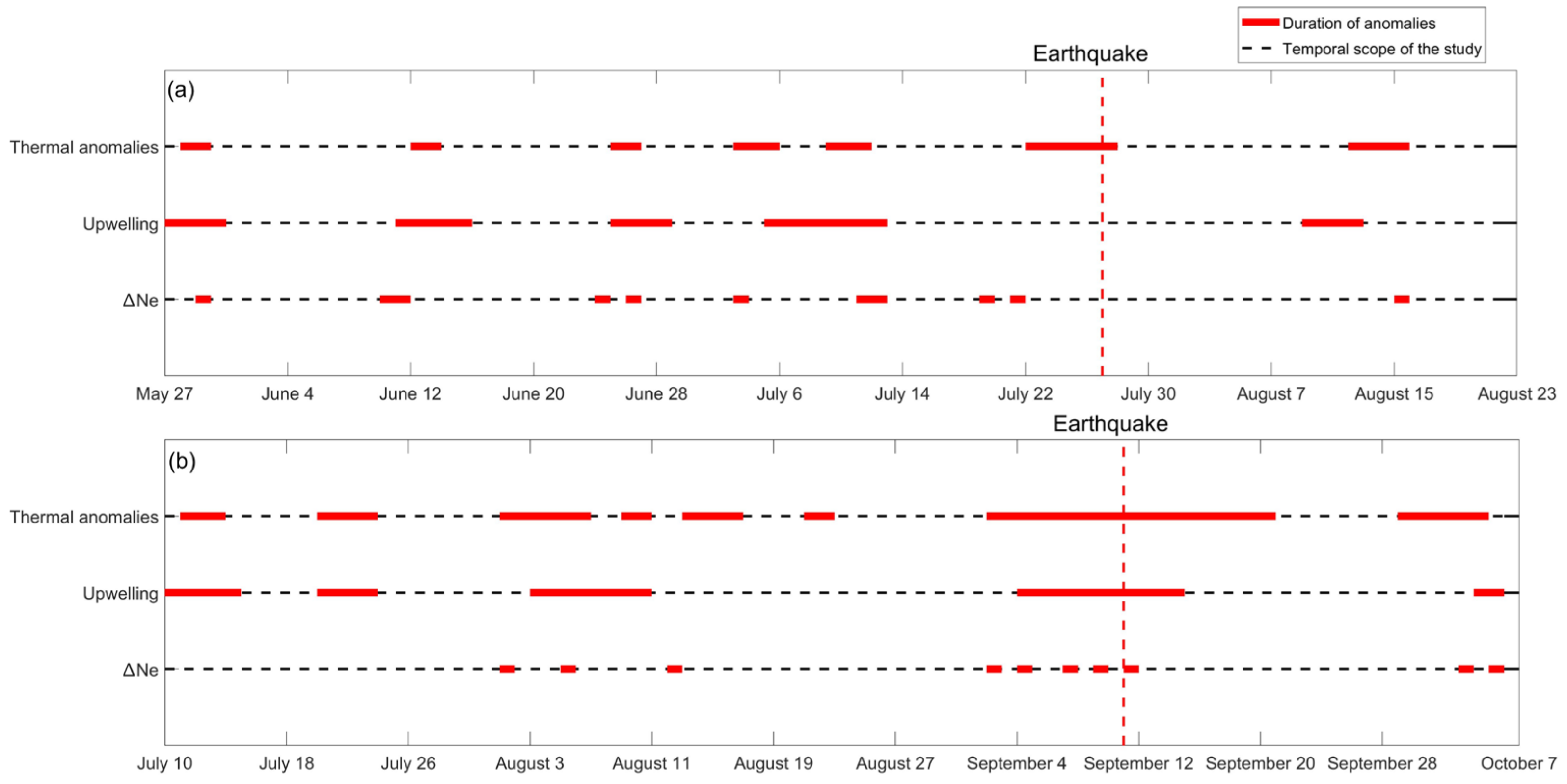
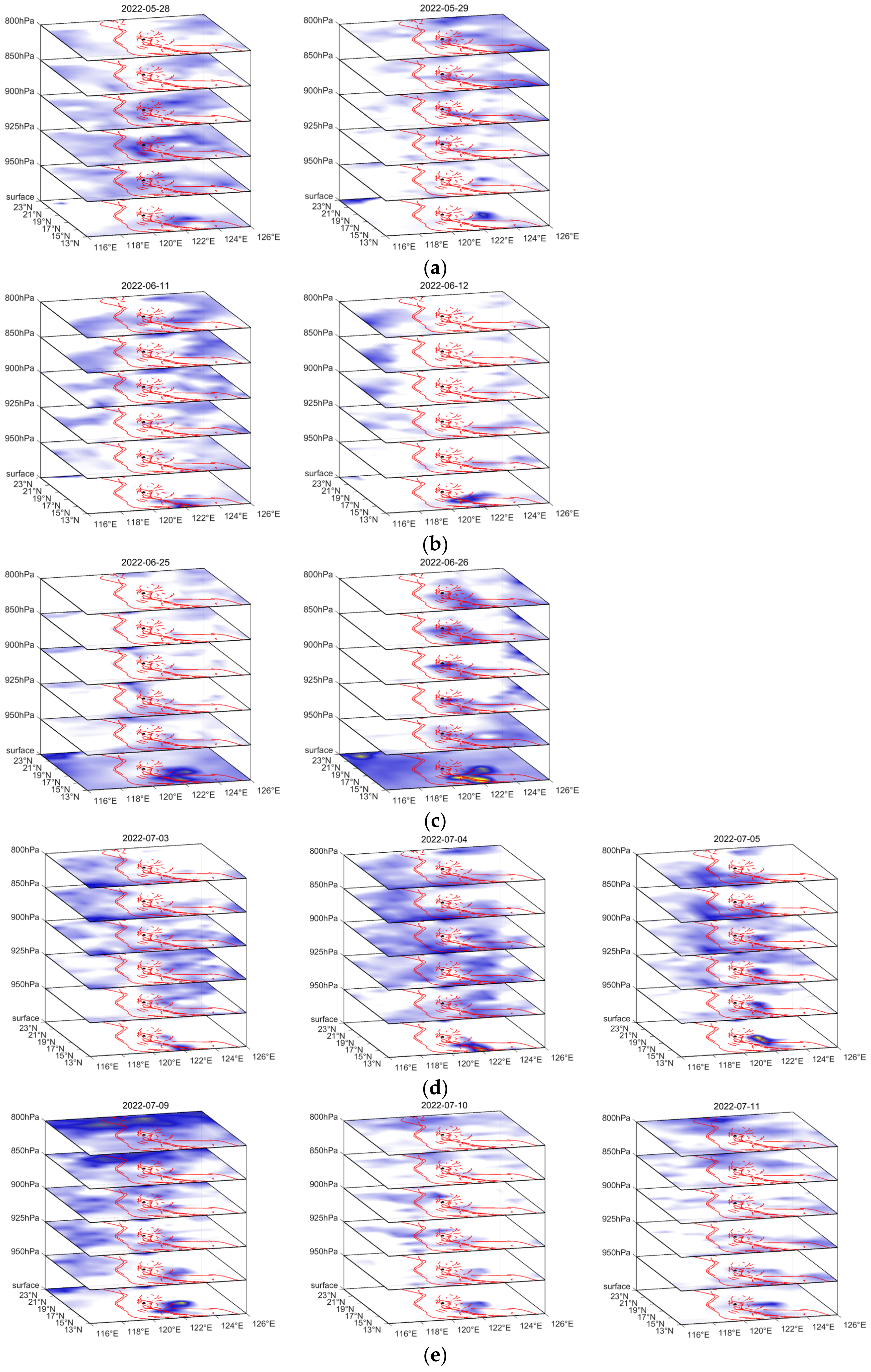
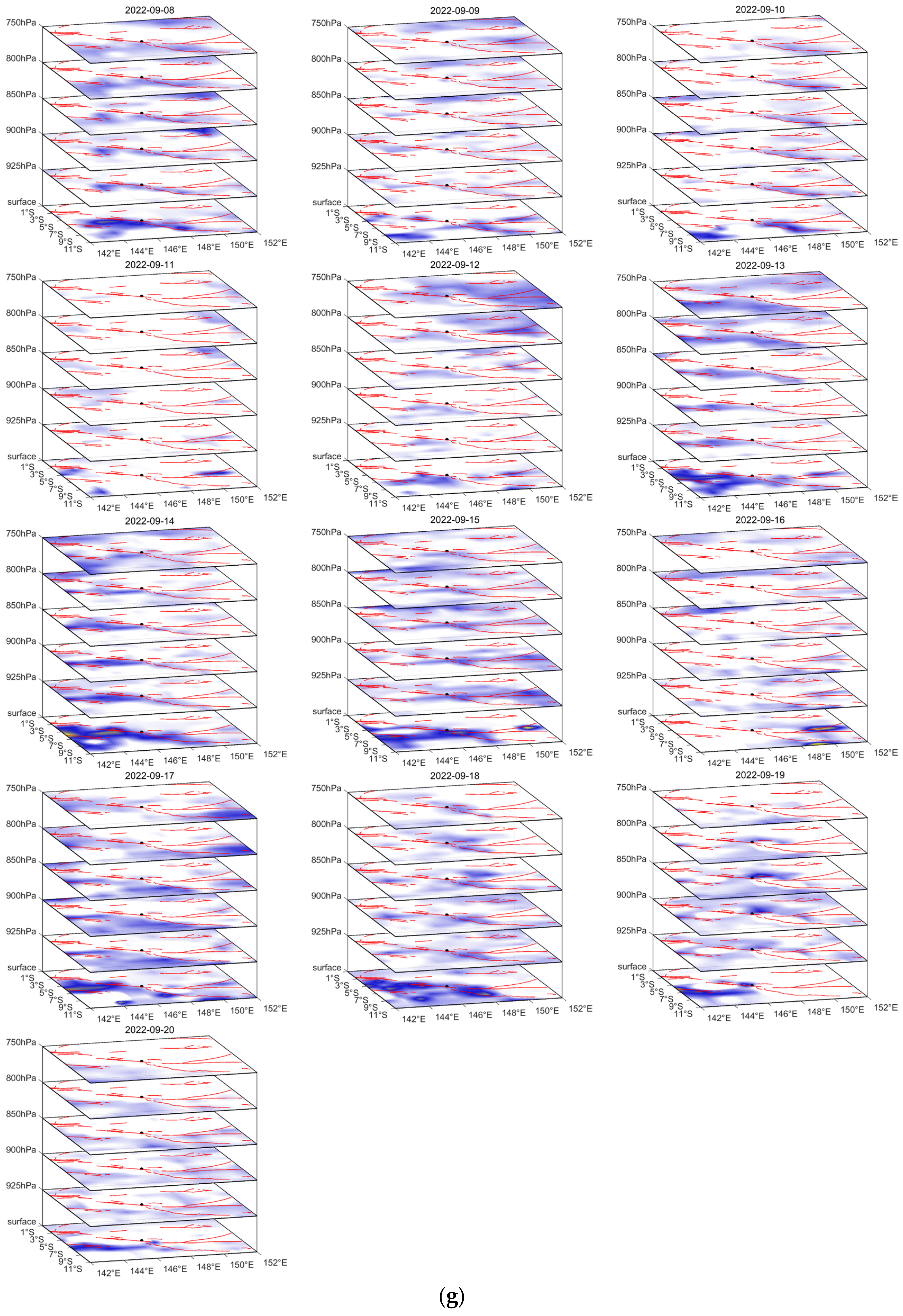
3.1. Seismic Thermal Anomalies

The temperature fluctuations at different isobaric levels throughout the analyzed time frames are depicted in the Supplementary Materials (Figures S1 and S2). Figure A1 and Figure A2 demonstrate the identified thermal anomalies related to the two earthquakes. We identified a total of seven seismic thermal anomalies spanning from 3 days to 6 days for the Mw = 7.0 earthquake, and eight seismic thermal anomalies ranging from 2 days to 19 days for the Mw = 7.6 earthquake, as listed in Table 2. It can be seen that the seismic thermal anomalies adhered to the sequential pattern of “initial rise-intensification-attenuation”, which correlates with the thermal infrared radiation process associated with rock fracturing under stress loading [45]. Other disorganized anomalies might arise from intricate meteorological activity and can be readily differentiated from seismic thermal anomalies based on their distinct patterns of variation and distribution [24]. The anomalies associated with the two earthquakes exhibited substantial variations in duration. The earthquakes (Mw = 7.0) with a smaller land area near the epicenter produced thermal anomalies that were temporally more dispersed compared to the earthquake (Mw = 7.6) with a larger land area near the epicenter. Similarly, the earthquake with an Mw = 7.6 magnitude generated broader and more intense anomalies on a spatial scale compared to the earthquake with an Mw = 7.0 magnitude. Additionally, the spatial evolution process demonstrated an intriguing tendency, wherein seismic thermal anomalies propagated from land towards the surrounding oceans.

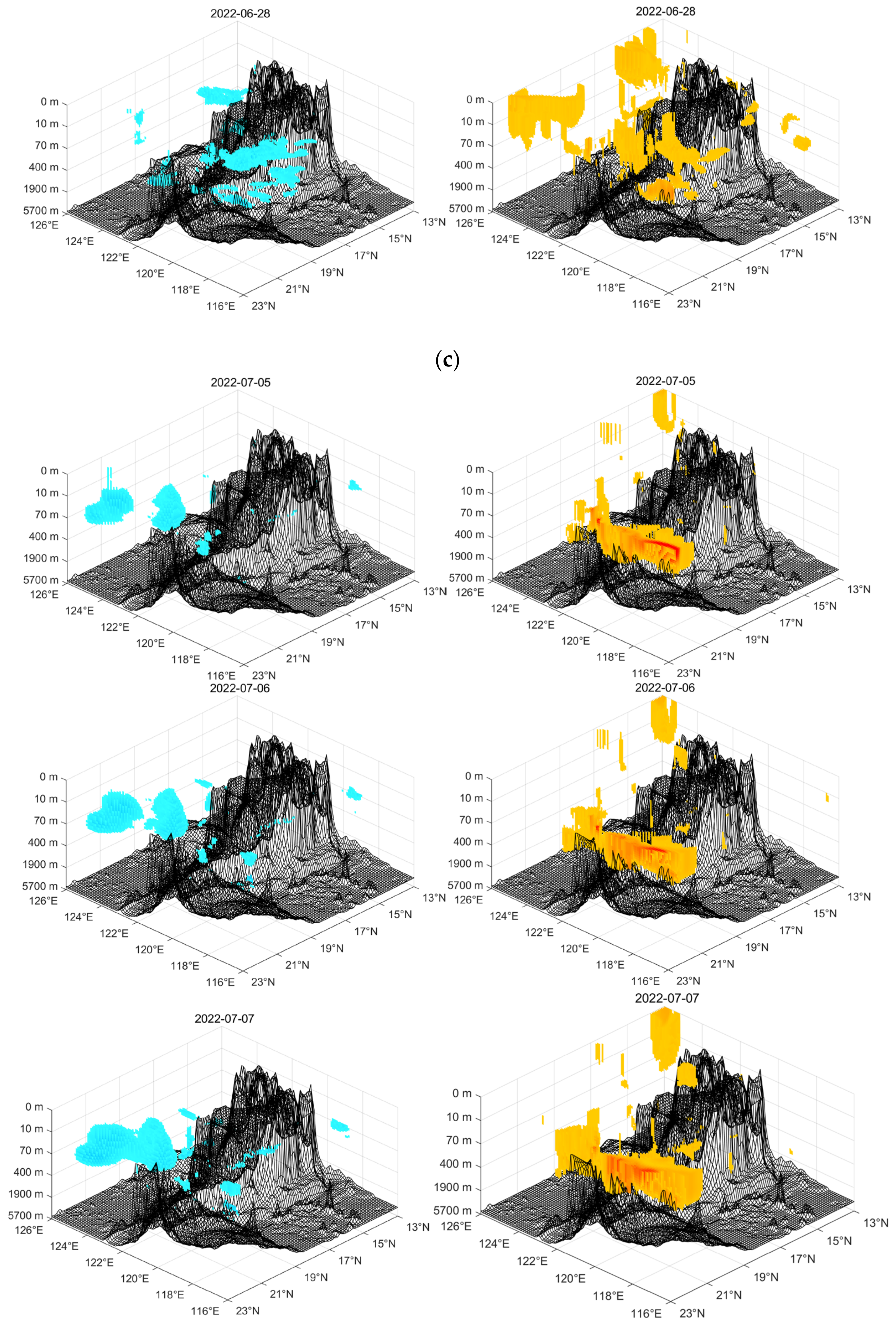
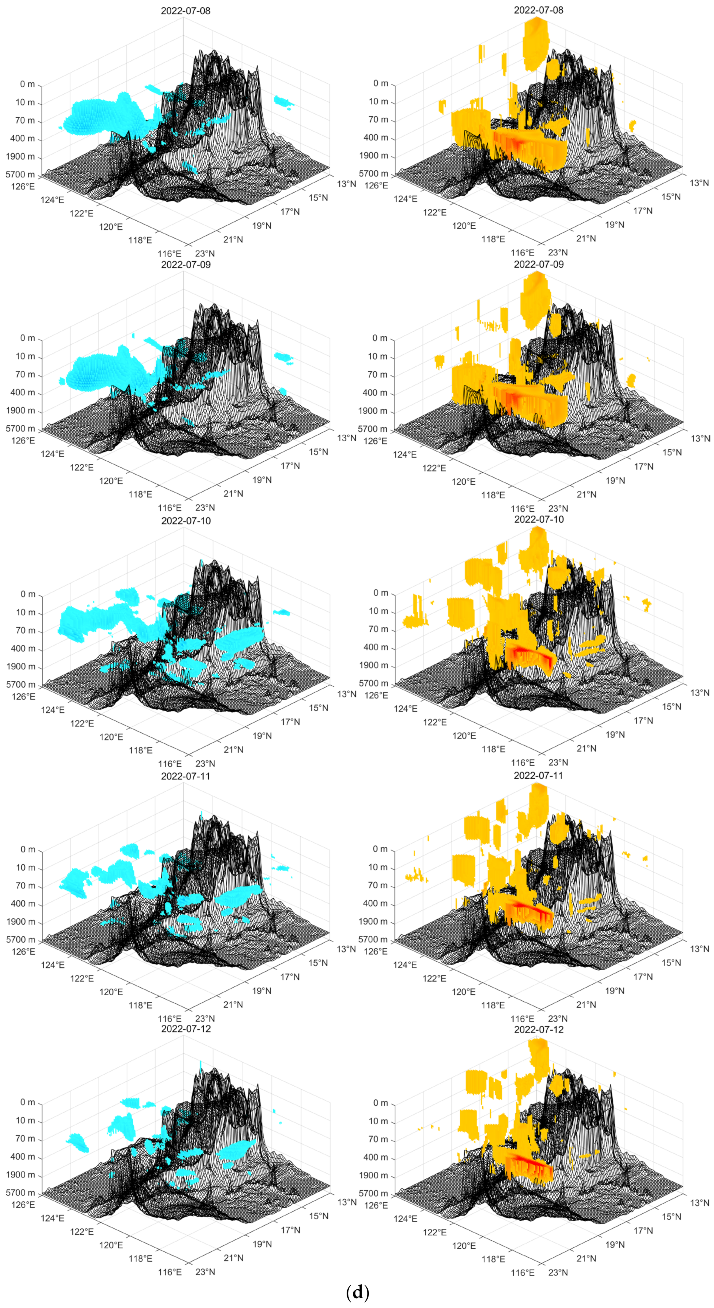
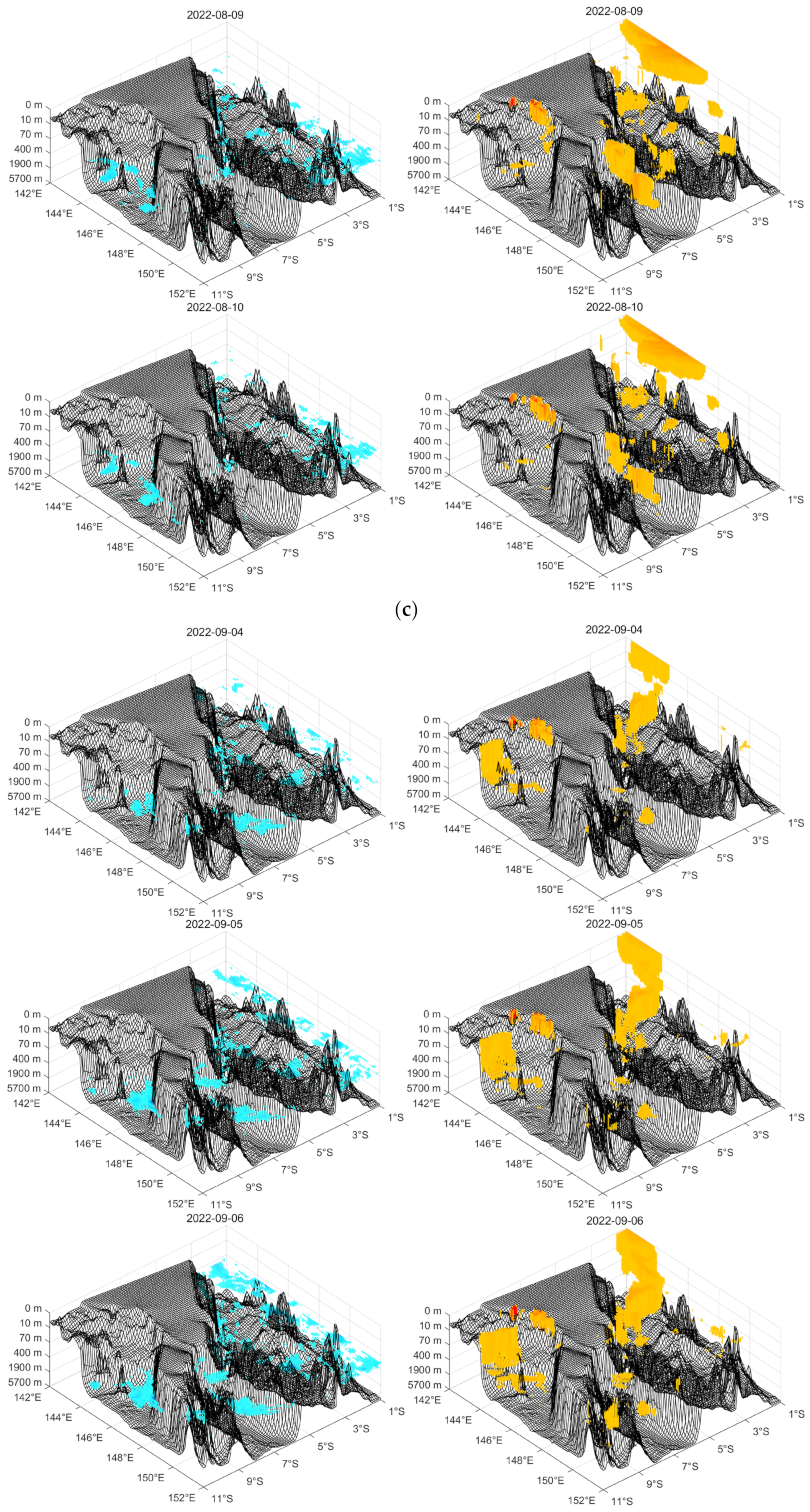
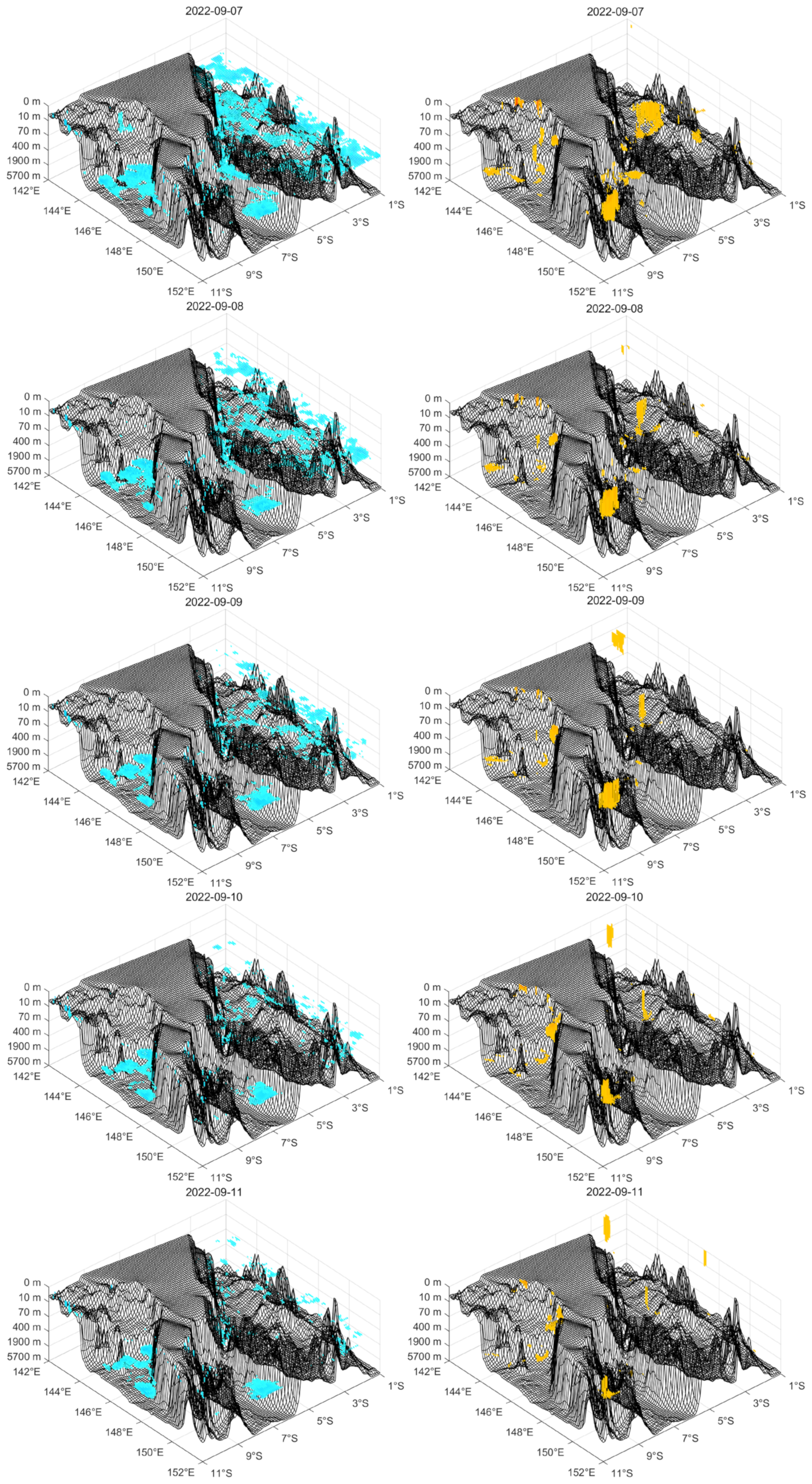
3.2. Sea Potential Temperature (SPT) and Sea Water Salinity (SWS)

3.2.1. Identification of Abnormal Upwelling

In order to offer robust evidence concerning oceanic anomalies associated with earthquakes and their interplay with atmospheric seismic thermal anomalies, we delved into the vertical evolution process of SPT and SWS subsequent to background removal via the TFFA method. In this study, we focused on the generation of upwelling in the ocean near the earthquake breeding zones. Therefore, the negative anomalies of SPT and the positive anomalies of SWS were identified for subsequent analysis. The comprehensive evolution process of two parameters for the Mw = 7.0 earthquake and Mw = 7.6 earthquake is shown in the Supporting Information (Figures S3–S6). Throughout the studied periods, we observed three patterns of SPT variation: (1) no anomalies emerging or weak anomalies emerging with a short spatial span; (2) anomalies emerging with variable strength and discontinuous distribution; (3) intense anomalies emerging with a trend of “intensification-peak-weakening” or “peak-weakening” in time, wide spatial span and continuous spatial distribution. The corresponding time ranges of the three anomalous variation patterns are shown in Table 3. It is evident that the third pattern exhibits a consistent trend of variation and pronounced spatial continuity, whereas the anomalous distribution of the first and second patterns appears obscure and irregular. Hence, further analysis was carried out on the third pattern, and the evolution process of SPT and SWS over the third pattern duration is shown in Figure A3 (Mw = 7.0 earthquake) and Figure A4 (Mw = 7.6 earthquake). The SWS anomalies maintain a high degree of concurrence with SPT anomalies for most of the third pattern. In particular, SWS anomalies manifest near or above the SPT anomalies, exhibiting a tendency of “intensification-peak-weakening” or “peak-weakening”. The simultaneous shifts in SPT decrease and SWS increase suggest that external driving forces are causing an uplift of deep water. As depicted in Figure A3, in the vicinity of the northern region (22°N, 116°S), a pronounced and enduring enhancement of SWS is spatially concentrated, which contrasts with the behavior of other anomalies. This is related to seasonal variation in summer; that is, the enhanced penetration of Kuroshio water via the Luzon Strait [46,47,48].

3.2.2. Confutation Analysis

The circulation in the ocean varies at seasonal time scales. Investigating the variation in SPT and SWS across different years within the same spatial range can contribute to confirming the distinctiveness of the upwelling generated before and after the two earthquakes. We conducted the TFFA on SPT and SWS for the vicinity of the two earthquakes during comparable time periods in 2021. Note that due to the intrinsic periodic nature of tidal force, the selection of an entirely congruent time range was unattainable. The time span from 6 June 2021 to 18 August 2021, encompassing five tidal force cycles, and the period from 20 July 2021 to 2 August 2021, spanning five tidal force cycles, were, respectively, employed as temporal windows for the confutation analysis pertaining to the two seismic events. Here, we present the key findings indicated by the confutation analysis (Figures S7–S10): (1) For the Mw = 7.0 earthquake, the SPT anomalies in 2021 were generally dispersed throughout most of the time period. An anomaly caused by force intruding from above was observed from July 16 to 18. Anomalies aligned with the aforementioned “the third pattern” occurred from July 20 to 23 and August 1 to 6, yet no corresponding increase in the salinity of overlying seawater at the same spatial locations was observed. This suggests that these anomalies are not induced by intense upwelling currents. Additionally, the enhanced SWS in the northern region was consistent with the results of 2022, further indicating its association with the enhanced penetration of Kuroshio water via the Luzon Strait. (2) For the Mw = 7.6 earthquake, the SPT anomalies were both dispersed and of relatively weak intensity for the majority of the time. Occasional SPT anomalies exhibited clustering tendencies, yet they dissipated swiftly within two to three days. Also, there was no apparent spatiotemporal synchrony observed with salinity anomalies. This provides evidence that the seasonal influence of oceanic currents consistently leads to anomalies during comparable timeframes across different years. In contrast, the intense and prolonged upwelling associated with earthquakes is distinct and distinguishable.

3.3. Vertical Electron Density Variation

In order to examine the vertical perturbations in the ionosphere associated with earthquakes, anomaly detection on Ne profiles was performed based on TFFA. Figure 4 illustrates the numerical distance between daily Δ Ne and boundaries within the examined timeframes for both the Mw = 7.0 earthquake and the Mw = 7.6 earthquake. Subsequently, we isolated the profiles that intersect the boundaries, as shown in Figure 5. In general, Δ Ne anomalies show an obvious aggregation phenomenon on the time scale. In particular, four short-term consecutive anomalies emerged in the case of the Mw = 7.0 earthquake (i.e., 10 June and 11 June, 24 June and 26 June, 11 July and 12 July, 19 July and 21 July). Also, two short-term consecutive anomalies and one long-term consecutive anomaly emerged in the case of the Mw = 7.6 earthquake (i.e., 1 August and 5 August, from 2 September to 11 September, 3 October and 5 October). It is interesting to notice that continuous anomalies aligned with one or both of the following variations: (1) profiles maintaining a similar shape and the amplitude of fluctuation increasing; (2) the peak moving to a higher altitude. This suggests that the ionospheric disturbance is enduring and propagates from lower to upper layers, with an evolutionary trajectory consistent with seismic thermal anomalies and upwelling driven by external forces. Additionally, conducting a comparative analysis of the temporal distribution is essential to demonstrate that the three types of anomalies do not occur in isolation.
Figure 6 shows the temporal distribution of anomalies across the ocean, lithosphere, atmosphere and ionosphere. Anomalies associated with the Mw = 7.6 earthquake exhibited stronger temporal continuity compared to those linked with the Mw = 7.0 earthquake. This contrast is particularly evident in the context of atmospheric thermal anomalies and ionospheric perturbations. The three types of anomalies exhibited notable temporal synchronization, with the majority of anomalies in the ocean and ionosphere occurring within the timeframe of thermal anomalies. Meanwhile, anomalies in the ocean tended to initiate around the same time as thermal anomalies. This observation implies a more profound intrinsic interrelation among the multi-layer disturbances induced by earthquakes.

4. Discussion

As an external factor, tidal force exerts an inducing impact on an active fault with tectonic stress in a critical state [21]. Both earthquakes studied, which occurred along coastal areas, took place three days after the tidal force peaked (Figure 1). This observation implies that tidal force might have played a substantial role in triggering the occurrence of these two major earthquakes. The seismic thermal anomalies observed recurred several times through the TFFA method. This is consistent with the reduplicative process of rock fracture and energy release [49,50,51]. However, the conspicuous temporal discontinuity of the thermal anomaly is a noteworthy aspect, with this discontinuity being more pronounced in the case of the Mw = 7.0 earthquake. Examining the specifics reveals that the ongoing enhancement and diffusion process is periodically disrupted by external factors, giving rise to short-term anomalies. For instance, during the Mw = 7.0 earthquake, the fourth thermal anomaly (from 3 July 2022 to 5 July 2022) and the fifth anomaly (from 9 July 2022 to 11 July 2022) exemplified this pattern. This interruption can be attributed to the environmental context of the studied earthquakes, particularly the relatively lower land-to-sea ratio.
The trend of thermal anomaly diffusion can provide additional support for further analysis. The seismic thermal anomalies associated with both earthquakes emanate from active faults situated on the land and in proximity, subsequently extending to the surrounding sea. This concurs with findings from alternative methodologies employed to detect seismic thermal anomalies [52,53,54]. The energy accumulation in seismogenic zones is dominated by squeezed rock under tectonic stress in active faults [55]. The process is intricately connected to the dynamic interplay of geological forces and convective thermal processes within the Earth’s subsurface. In this scenario, convective thermal fluids transform into thermal water vapor, gaseous emissions and heat flux. These elements ascend along geological structures and eventually reach the surface, subsequently leading to an increase in ground surface temperature, which signifies the presence of this process [12,56,57], as shown in Figure 7. The origin of atmospheric seismic thermal anomalies lies in the increased surface temperature over land. Consequently, the discernibility of thermal anomalies can be hindered by various overlapping environmental influences. The smaller land area renders anomalies less intense and more susceptible to interference.
In contrast to anomalies observed on the surface and in the atmosphere, the seismic anomalies within the ocean display analogous evolutionary patterns, yet distinctive manifestations. We observed SPT and SWS anomalies in the two earthquakes, most of which occurred within the duration of seismic thermal anomalies. The synchronous process of the decreasing SPT and increasing SWS indicated that the deep water was uplifted by external driving forces, resulting in the formation of upwelling. These occurrences were accompanied by unique time frames and spatial spans of observed upwelling. For the Mw = 7.0 earthquake, frequent upwelling was concentrated around the epicenter (northwestern Luzon island) between June and August, with higher intensity observed in the northern regions. The coastal upwelling along the northern shores of Luzon Island was predominantly influenced by a cold eddy known as the Luzon cold eddy [58]. This cyclonic eddy was detected using multiple data, including long-term observational data in the South China Sea [59], temperature and salinity data [60,61] and altimeter data [62]. Analysis reveals that this eddy followed a distinct “development-intensification-decay” pattern from October to the subsequent May [58]. In the case of the Mw = 7.6 earthquake, upwelling was reduplicative and continuous in the Bismarck Sea and the Solomon Sea from July to September. During July and August, the temperature and salinity patterns in the Bismarck Sea and Solomon Sea were predominantly influenced by horizontal advection rather than upwelling. In contrast, in January and February, coastal upwelling driven by northwest monsoon winds significantly impacted temperature and salinity dynamics [63]. The confutation analysis yielded evidence of consistent seasonal anomalies induced by oceanic currents within comparable timeframes across different years, while in contrast, distinct and prolonged upwelling events linked to earthquakes were discernible. Hence, the upwelling events before and after earthquakes exhibited distinct features and were attributed to seismic driving mechanisms. Furthermore, the upwelling was distributed in a north–south direction near the epicenter of the Mw = 7.0 earthquake, while its diffusion in the east–west direction was not apparent. Conversely, the upwelling observed near the epicenter of the Mw = 7.6 earthquake demonstrated a tendency to propagate in an east–west direction. This spatial distribution corresponded to the adjacent tectonic plate boundaries near the epicenters (Figure 1). Therefore, the spatial distribution, temporal progression and evolution pattern of SPT and SWS anomalies suggest that the earthquake preparation process impacts the ocean dynamics (Figure 7). This effect is manifested by the energy imparted to the ocean floor during the acceleration of tectonic plates into subduction, subsequently leading to the uplifting of colder water.
The soundings provided by F7/C2 had a relatively dense distribution and covered land and ocean, thereby unveiling intriguing vertical variations in seismic perturbations in the ionosphere. The anomalies, emerging from a few days to approximately 60 days before earthquakes, coincided with ionospheric perturbations related to earthquakes detected by alternative data and methodologies [64,65,66]. Most Ne anomalies occur in the duration of seismic thermal anomalies, consistent with our past research [24]. We noticed that continuous Ne anomalies exhibited an increasing amplitude or an upward shift in the peak. This vertical structure change reflects the same bottom-up disturbances as the seismic thermal anomalies. Additionally, similar to the interruption observed in the analysis of seismic thermal anomalies discussed earlier and its correlation with earthquakes occurring in regions with smaller land area, analogous patterns were also discernible in ionospheric seismic anomalies. In comparison to the Mw = 7.0 earthquake, the Mw = 7.6 earthquake was characterized by a higher ratio of land to sea, resulting in a more concentrated occurrence of Ne anomalies. These observations substantiate the significant correlation between ionospheric disturbances induced by earthquakes and seismic thermal anomalies. The heating of the lower isobaric level from the ground surface produces an air pressure gradient [23]. The pressure gradient propagates toward the upper atmosphere and disturbs the ionosphere [67,68,69].
In light of the above analysis, the clear anomalous propagation pattern that enhances the understanding of OLAIC has been interconnected and presented, as illustrated in Figure 7. Furthermore, seismic anomalies across the ocean, lithosphere, atmosphere and ionosphere were effectively identified through tidal force fluctuation, substantiating their coupled relationship. In previous studies, tidal force fluctuation has only been used to detect seismic anomalies in the atmosphere and on the surface [16,21,22,23,24]. Through amalgamating multi-source data and employing refined parameter criteria, tidal force fluctuation has the potential to emerge as a viable approach for delineating ocean–lithosphere–atmosphere–ionosphere coupling (OLAIC).

5. Conclusions

In the current investigation, we explored coupling anomalies in the ocean, atmosphere and ionosphere through tidal force fluctuation based on oceanic parameters (i.e., sea potential temperature and sea water salinity), air temperature and electron density profiles. The findings reveal that the intensity of seismic anomalies in the atmosphere is influenced by the land-to-sea ratio near the epicenter. Seismic thermal anomalies initiate along the active faults and adhere to the pattern of change characterized by ‘initial rise-intensification-attenuation’, attributed to the thermal radiation resulting from rock fracture. Similarly, seismic upwelling, driven by the uplift of cold water, propagates along plate boundaries with a discernible ‘intensification-peak-weakening’ trend under the action of the accelerated subduction of tectonic plates. The evolution process and temporal discontinuity of seismic thermal anomalies and electron density (Ne) anomalies suggest a potential link between ionospheric perturbations and atmospheric pressure gradients. The occurrence of Ne anomalies and seismic upwelling is effectively encompassed within the duration of seismic thermal anomalies, and there is a synchronous evolution tendency among multi-layers. This collective behavior offers insights into ocean–lithosphere–atmosphere–ionosphere coupling (OLAIC) and the intricate transmission of anomalies associated with earthquakes that occur on the sea coast. During earthquake preparation phases, the acceleration of plate subduction leads to two main processes: (1) The energy released by rock fracture under enhanced tectonic stress in active faults acts on convective thermal fluids. Subsequently, the fluid breaks down, rises and heats the land surface, causing atmospheric thermal anomalies, creating the air pressure gradient that disturbs the ionosphere. (2) The energy deposited into the ocean floor along the plate boundaries uplifts cold water to drive upwelling, which promotes a decline in potential temperature and an increase in the salinity in the upper ocean. Furthermore, the tidal force fluctuation method, which is excellent in the identification of multi-layer anomalies, is worthy of further study.

Supplementary Materials

The following supporting information can be downloaded at: https://www.mdpi.com/article/10.3390/rs15184392/s1, Figure S1: Air temperature change in (a) tidal force period A, (b) tidal force period B, (c) tidal force period C, (d) tidal force period D, (e) tidal force period E and (f) tidal force period F for Mw = 7.0 earthquake. The epicenter and faults are shown by black point and red lines, respectively; Figure S2: Air temperature change in (a) tidal force period A, (b) tidal force period B, (c) tidal force period C, (d) tidal force period D, (e) tidal force period E and (f) tidal force period F for Mw = 7.6 earthquake. The epicenter and faults are shown by black point and red lines, respectively; Figure S3: The variation of sea potential temperature anomalies during the studies periods for Mw = 7.0 earthquake; Figure S4: The variation of sea potential temperature anomalies during the studies periods for Mw = 7.6 earthquake; Figure S5: The variation of sea water salinity anomalies during the studies periods for Mw = 7.0 earthquake; Figure S6: The variation of sea water salinity anomalies during the studies periods for Mw = 7.6 earthquake; Figure S7: The variation of sea potential temperature anomalies from 6 June 2021 to 18 August 2021 within 13–23°N and 116–126°E; Figure S8: The variation of sea potential temperature anomalies from 20 July 2021 to 2 October 2021 within 11–1°S and 142–152°E; Figure S9: The variation of sea water salinity anomalies from 6 June 2021 to 18 August 2021 within 13–23°N and 116–126°E; Figure S10: The variation of sea water salinity anomalies from 20 July 2021 to 2 October 2021 within 11–1°S and 142–152°E.

Author Contributions

Conceptualization, X.X.; methodology, X.X.; software, X.X.; validation, X.X., L.W.; formal analysis, X.X.; investigation, X.X.; resources, X.X.; data curation, X.X.; writing—original draft preparation, X.X.; writing—review and editing, S.C., L.W.; visualization, X.X.; supervision, S.C.; project administration, S.C. All authors have read and agreed to the published version of the manuscript.

Funding

This research was funded by China Scholarship Council (CSC).

Data Availability Statement

The earthquake data are available at USGS (https://earthquake.usgs.gov/earthquakes, accessed on 7 August 2023). The air temperature data are available at NCAR (https://rda.ucar.edu/datasets/ds083.2/, accessed on 7 August 2023). The sea potential temperature data and seawater salinity data are available at CNEMS (https://data.marine.copernicus.eu/products, accessed on 29 August 2023). The FORMOSAT-7/COSMIC-2 soundings are available at TACC (tacc.cwb.gov.tw/v2/trops_download.html, accessed on 7 August 2023).

Acknowledgments

The authors express gratitude to NCEP for supplying air temperature data and to the CNEMS community for sharing oceanic data. The authors also extend their appreciation to TACC for sharing electron density data and to USGS for providing earthquake data.

Conflicts of Interest

The authors declare no conflict of interest.

Appendix A

The evolution processes of seismic thermal anomalies of the two earthquakes are shown in Figure A1 and Figure A2.
Figure A1. Seismic thermal anomalies that occurred (a) from 28 May to 29 May, (b) from 11 June to 12 June, (c) from 25 June to 26 June, (d) from 3 July to 5 July, (e) from 9 July to 11 July, (f) from 22 July to 27 July and (g) from 12 August to 15 August.
Remotesensing 15 04392 g0a1aRemotesensing 15 04392 g0a1b
Figure A2. Seismic anomalies that occurred (a) from 11 July to 13 July, (b) from 20 July to 23 July, (c) from 1 August to 6 August, (d) from 9 August to 10 August, (e) from 13 August to 16 August, (f) 21 August to 22 August, (g) 2 September to 20 September and (h) 29 September to 4 October.
Remotesensing 15 04392 g0a2aRemotesensing 15 04392 g0a2bRemotesensing 15 04392 g0a2cRemotesensing 15 04392 g0a2dRemotesensing 15 04392 g0a2e

Appendix B

The evolution processes of SPT anomalies and SWS anomalies over the third pattern duration of the two earthquakes are shown in Figure A3 and Figure A4.
Figure A3. The third anomalous variation pattern of sea potential temperature and corresponding anomalous variation in seawater salinity (a) from 27 May to 30 May, (b) from 11 June to 15 June, (c) from 25 June to 28 June, (d) from 5 July to 12 July and (e) from 9 August to 12 August.
Remotesensing 15 04392 g0a3aRemotesensing 15 04392 g0a3bRemotesensing 15 04392 g0a3cRemotesensing 15 04392 g0a3dRemotesensing 15 04392 g0a3eRemotesensing 15 04392 g0a3f
Figure A4. The third anomalous variation pattern of sea potential temperature and corresponding anomalous variations in seawater salinity (a) from 10 July to 14 July, (b) 20 July to 23 July, (c) from 3 August to 10 August, (d) from 4 September to 14 September and (e) from 4 October to 5 October.
Remotesensing 15 04392 g0a4aRemotesensing 15 04392 g0a4bRemotesensing 15 04392 g0a4cRemotesensing 15 04392 g0a4dRemotesensing 15 04392 g0a4eRemotesensing 15 04392 g0a4fRemotesensing 15 04392 g0a4g

References

  1. Davidenko, D.; Pulinets, S. Deterministic variability of the ionosphere on the eve of strong (M ≥ 6) earthquakes in the regions of Greece and Italy according to long-term measurements data. Geomagn. Aeron. 2019, 59, 493–508. [Google Scholar] [CrossRef]
  2. Shah, M.; Tariq, M.A.; Ahmad, J.; Naqvi, N.A.; Jin, S. Seismo ionospheric anomalies before the 2007 M7. 7 Chile earthquake from GPS TEC and DEMETER. J. Geodyn. 2019, 127, 42–51. [Google Scholar] [CrossRef]
  3. Choudhury, S.; Dasgupta, S.; Saraf, A.K.; Panda, S. Remote sensing observations of pre-earthquake thermal anomalies in Iran. Int. J. Remote Sens. 2006, 27, 4381–4396. [Google Scholar] [CrossRef]
  4. Cui, Y.; Ouzounov, D.; Hatzopoulos, N.; Sun, K.; Zou, Z.; Du, J. Satellite observation of CH4 and CO anomalies associated with the Wenchuan MS 8.0 and Lushan MS 7.0 earthquakes in China. Chem. Geol. 2017, 469, 185–191. [Google Scholar] [CrossRef]
  5. Chakraborty, S.; Sasmal, S.; Basak, T.; Chakrabarti, S.K. Comparative study of charged particle precipitation from Van Allen radiation belts as observed by NOAA satellites during a land earthquake and an ocean earthquake. Adv. Space Res. 2019, 64, 719–732. [Google Scholar] [CrossRef]
  6. Singh, R.P.; Dey, S.; Bhoi, S.; Sun, D.; Cervone, G.; Kafatos, M. Anomalous increase of chlorophyll concentrations associated with earthquakes. Adv. Space Res. 2006, 37, 671–680. [Google Scholar] [CrossRef]
  7. Genzano, N.; Filizzola, C.; Hattori, K.; Pergola, N.; Tramutoli, V. Statistical correlation analysis between thermal infrared anomalies observed from MTSATs and large earthquakes occurred in Japan (2005–2015). J. Geophys. Res. Solid Earth 2021, 126, e2020JB020108. [Google Scholar] [CrossRef]
  8. Adil, M.A.; Şentürk, E.; Pulinets, S.A.; Amory-Mazaudier, C. A lithosphere–atmosphere–ionosphere coupling phenomenon observed before M 7.7 Jamaica Earthquake. Pure Appl. Geophys. 2021, 178, 3869–3886. [Google Scholar] [CrossRef]
  9. Mehdi, S.; Shah, M.; Naqvi, N.A. Lithosphere atmosphere ionosphere coupling associated with the 2019 M w 7.1 California earthquake using GNSS and multiple satellites. Environ. Monit. Assess. 2021, 193, 501. [Google Scholar] [CrossRef]
  10. Shah, M.; Aibar, A.C.; Tariq, M.A.; Ahmed, J.; Ahmed, A. Possible ionosphere and atmosphere precursory analysis related to Mw> 6.0 earthquakes in Japan. Remote Sens. Environ. 2020, 239, 111620. [Google Scholar] [CrossRef]
  11. Jing, F.; Singh, R.P.; Shen, X. Land–atmosphere–meteorological coupling associated with the 2015 Gorkha (M 7.8) and Dolakha (M 7.3) Nepal earthquakes. Geomat. Nat. Hazards Risk 2019, 10, 1267–1284. [Google Scholar] [CrossRef]
  12. Pulinets, S.; Ouzounov, D. Lithosphere–Atmosphere–Ionosphere Coupling (LAIC) model–An unified concept for earthquake precursors validation. J. Asian Earth Sci. 2011, 41, 371–382. [Google Scholar] [CrossRef]
  13. Freund, F. Pre-earthquake signals: Underlying physical processes. J. Asian Earth Sci. 2011, 41, 383–400. [Google Scholar] [CrossRef]
  14. Kuo, C.; Huba, J.; Joyce, G.; Lee, L. Ionosphere plasma bubbles and density variations induced by pre-earthquake rock currents and associated surface charges. J. Geophys. Res. Space Phys. 2011, 116, A10317. [Google Scholar] [CrossRef]
  15. Kuo, C.; Lee, L.; Huba, J. An improved coupling model for the lithosphere-atmosphere-ionosphere system. J. Geophys. Res. Space Phys. 2014, 119, 3189–3205. [Google Scholar] [CrossRef]
  16. Weiyu, M.; Xuedong, Z.; Liu, J.; Yao, Q.; Zhou, B.; Yue, C.; Kang, C.; Lu, X. Influences of multiple layers of air temperature differences on tidal forces and tectonic stress before, during and after the Jiujiang earthquake. Remote Sens. Environ. 2018, 210, 159–165. [Google Scholar] [CrossRef]
  17. Tramutoli, V. Robust satellite techniques (RST) for natural and environmental hazards monitoring and mitigation: Theory and applications. In Proceedings of the 2007 International Workshop on the Analysis of Multi-Temporal Remote Sensing Images, Leuven, Belgium, 18–20 July 2007; pp. 1–6. [Google Scholar]
  18. Ouzounov, D.; Pulinets, S.; Romanov, A.; Romanov, A.; Tsybulya, K.; Davidenko, D.; Kafatos, M.; Taylor, P. Atmosphere-ionosphere response to the M 9 Tohoku earthquake revealed by multi-instrument space-borne and ground observations: Preliminary results. Earthq. Sci. 2011, 24, 557–564. [Google Scholar] [CrossRef]
  19. Xiong, P.; Shen, X. Outgoing longwave radiation anomalies analysis associated with different types of seismic activity. Adv. Space Res. 2017, 59, 1408–1415. [Google Scholar] [CrossRef]
  20. Tramutoli, V.; Corrado, R.; Filizzola, C.; Genzano, N.; Lisi, M.; Pergola, N. From visual comparison to Robust Satellite Techniques: 30 years of thermal infrared satellite data analyses for the study of earthquake preparation phases. Boll. Geofis. Teor. Appl. 2015, 56, 167–202. [Google Scholar]
  21. Zhang, X.; Kang, C.; Ma, W.; Ren, J.; Wang, Y. Study on thermal anomalies of earthquake process by using tidal-force and outgoing-longwave-radiation. Therm. Sci. 2018, 22, 767–776. [Google Scholar] [CrossRef]
  22. Zhang, Y.; Meng, Q.; Wang, Z.; Lu, X.; Hu, D. Temperature variations in multiple air layers before the Mw 6.2 2014 Ludian earthquake, Yunnan, China. Remote Sens. 2021, 13, 884. [Google Scholar] [CrossRef]
  23. Xu, X.; Chen, S.; Yu, Y.; Zhang, S. Atmospheric anomaly analysis related to Ms> 6.0 earthquakes in China during 2020–2021. Remote Sens. 2021, 13, 4052. [Google Scholar] [CrossRef]
  24. Xu, X.; Chen, S.; Zhang, S.; Dai, R. Analysis of Potential Precursory Pattern at Earth Surface and the Above Atmosphere and Ionosphere Preceding Two Mw≥ 7 Earthquakes in Mexico in 2020–2021. Earth Space Sci. 2022, 9, e2022EA002267. [Google Scholar] [CrossRef]
  25. Heaton, T.H. Tidal triggering of earthquakes. Geophys. J. Int. 1975, 43, 307–326. [Google Scholar] [CrossRef]
  26. Su, Y.-C.; Liu, J.-Y.; Chen, S.-P.; Tsai, H.-F.; Chen, M.-Q. Temporal and spatial precursors in ionospheric total electron content of the 16 October 1999 Mw7. 1 Hector Mine earthquake. J. Geophys. Res. Space Phys. 2013, 118, 6511–6517. [Google Scholar] [CrossRef]
  27. Yan, X.; Sun, Y.; Yu, T.; Liu, J.Y.; Qi, Y.; Xia, C.; Zuo, X.; Yang, N. Stratosphere perturbed by the 2011 Mw9. 0 Tohoku earthquake. Geophys. Res. Lett. 2018, 45, 10050–10056. [Google Scholar] [CrossRef]
  28. Ahmed, J.; Shah, M.; Zafar, W.A.; Amin, M.A.; Iqbal, T. Seismoionospheric anomalies associated with earthquakes from the analysis of the ionosonde data. J. Atmos. Sol. Terr. Phys. 2018, 179, 450–458. [Google Scholar] [CrossRef]
  29. Dey, S.; Singh, R. Surface latent heat flux as an earthquake precursor. Nat. Hazards Earth Syst. Sci. 2003, 3, 749–755. [Google Scholar] [CrossRef]
  30. Ouzounov, D.; Freund, F. Mid-infrared emission prior to strong earthquakes analyzed by remote sensing data. Adv. Space Res. 2004, 33, 268–273. [Google Scholar] [CrossRef]
  31. Okada, Y.; Mukai, S.; Singh, R. Changes in atmospheric aerosol parameters after Gujarat earthquake of January 26, 2001. Adv. Space Res. 2004, 33, 254–258. [Google Scholar] [CrossRef]
  32. Akhoondzadeh, M. Ant Colony Optimization detects anomalous aerosol variations associated with the Chile earthquake of 27 February 2010. Adv. Space Res. 2015, 55, 1754–1763. [Google Scholar] [CrossRef]
  33. Zhang, L.; Jiang, M.; Jing, F. Sea temperature variation associated with the 2021 Haiti M w 7.2 earthquake and possible mechanism. Geomat. Nat. Hazards Risk 2022, 13, 2840–2863. [Google Scholar] [CrossRef]
  34. Alvan, H.V.; Azad, F.H.; Omar, H.B. Chlorophyll concentration and surface temperature changes associated with earthquakes. Nat. Hazards 2012, 64, 691–706. [Google Scholar] [CrossRef]
  35. Mohamed, E.K.; Elrayess, M.; Omar, K. Evaluation of thermal anomaly preceding northern red sea earthquake, the 16th June 2020. Arab. J. Sci. Eng. 2022, 47, 7387–7406. [Google Scholar] [CrossRef]
  36. Liu, Y.; Wu, L.; Qi, Y.; Ding, Y. Very-Short-Term Variations of Sea Surface and Atmospheric Parameters Before the Ms 6.2 Zhangbei (China) Earthquake in 1998. Front. Environ. Sci. 2022, 10, 906455. [Google Scholar] [CrossRef]
  37. Lellouche, J.; Legalloudec, O.; Regnier, C.; Levier, B.; Greiner, E.; Drevillon, M. Quality Information Document for Globa L Sea Physical Analysis and Forecasting Product, Global_Analysis_ForecaST_PHY_001_024; EU Copernicus Marine Service European Union: Brussels, Belgium, 2019; Volume 81. [Google Scholar]
  38. Kalnay, E.; Kanamitsu, M.; Kistler, R.; Collins, W.; Deaven, D.; Gandin, L.; Iredell, M.; Saha, S.; White, G.; Woollen, J. The NCEP/NCAR 40-year reanalysis project. Bull. Am. Meteorol. Soc. 1996, 77, 437–472. [Google Scholar] [CrossRef]
  39. Kistler, R.; Kalnay, E.; Collins, W.; Saha, S.; White, G.; Woollen, J.; Chelliah, M.; Ebisuzaki, W.; Kanamitsu, M.; Kousky, V. The NCEP/NCAR 50-year reanalysis: Documentation and monthly-means CD-ROM. Bull. Am. Meteorol. Soc 2001, 82, 247–268. [Google Scholar] [CrossRef]
  40. Sun, Y.-Y.; Chen, C.-H.; Lin, C.-Y. Detection of vertical changes in the ionospheric electron density structures by the radio occultation technique onboard the FORMOSAT-7/COSMIC2 mission over the eruption of the Tonga underwater volcano on 15 January 2022. Remote Sens. 2022, 14, 4266. [Google Scholar] [CrossRef]
  41. Davies, K. Ionospheric Radio; IET: London, UK, 1990. [Google Scholar]
  42. Wang, J.; Sun, Y.Y.; Yu, T.; Wang, Y.; Mao, T.; Yang, H.; Xia, C.; Yan, X.; Yang, N.; Huang, G. Convergence effects on the ionosphere during and after the annular solar eclipse on 21 June 2020. J. Geophys. Res. Space Phys. 2022, 127, e2022JA030471. [Google Scholar] [CrossRef]
  43. Kilston, S.; Knopoff, L. Lunar–solar periodicities of large earthquakes in southern California. Nature 1983, 304, 21–25. [Google Scholar] [CrossRef]
  44. Dobrovolsky, I.; Zubkov, S.; Miachkin, V. Estimation of the size of earthquake preparation zones. Pure Appl. Geophys. 1979, 117, 1025–1044. [Google Scholar] [CrossRef]
  45. Wu, L.; Liu, S.; Wu, Y.; Wang, C. Precursors for rock fracturing and failure—Part II: IRR T-Curve abnormalities. Int. J. Rock Mech. Min. Sci. 2006, 43, 483–493. [Google Scholar] [CrossRef]
  46. Qu, T.; Mitsudera, H.; Yamagata, T. Intrusion of the north Pacific waters into the South China Sea. J. Geophys. Res. Ocean. 2000, 105, 6415–6424. [Google Scholar] [CrossRef]
  47. Dong, L.; Qi, J.; Yin, B.; Zhi, H.; Li, D.; Yang, S.; Wang, W.; Cai, H.; Xie, B. Reconstruction of Subsurface Salinity Structure in the South China Sea Using Satellite Observations: A LightGBM-Based Deep Forest Method. Remote Sens. 2022, 14, 3494. [Google Scholar] [CrossRef]
  48. Yi, D.L.; Melnichenko, O.; Hacker, P.; Potemra, J. Remote sensing of sea surface salinity variability in the South China Sea. J. Geophys. Res. Ocean. 2020, 125, e2020JC016827. [Google Scholar] [CrossRef]
  49. Tronin, A.A.; Hayakawa, M.; Molchanov, O.A. Thermal IR satellite data application for earthquake research in Japan and China. J. Geodyn. 2002, 33, 519–534. [Google Scholar] [CrossRef]
  50. Panda, S.; Choudhury, S.; Saraf, A.K.; Das, J.D. MODIS land surface temperature data detects thermal anomaly preceding 8 October 2005 Kashmir earthquake. Int. J. Remote Sens. 2007, 28, 4587–4596. [Google Scholar] [CrossRef]
  51. Fu, C.-C.; Lee, L.-C.; Ouzounov, D.; Jan, J.-C. Earth’s outgoing longwave radiation variability prior to M≥ 6.0 earthquakes in the Taiwan area during 2009–2019. Front. Earth Sci. 2020, 8, 364. [Google Scholar] [CrossRef]
  52. Zoran, M. MODIS and NOAA-AVHRR l and surface temperature data detect a thermal anomaly preceding the 11 March 2011 Tohoku earthquake. Int. J. Remote Sens. 2012, 33, 6805–6817. [Google Scholar] [CrossRef]
  53. Genzano, N.; Filizzola, C.; Paciello, R.; Pergola, N.; Tramutoli, V. Robust Satellite Techniques (RST) for monitoring earthquake prone areas by satellite TIR observations: The case of 1999 Chi-Chi earthquake (Taiwan). J. Asian Earth Sci. 2015, 114, 289–298. [Google Scholar] [CrossRef]
  54. Wu, L.; Zheng, S.; De Santis, A.; Qin, K.; Di Mauro, R.; Liu, S.; Rainone, M.L. Geosphere coupling and hydrothermal anomalies before the 2009 M w 6.3 L’Aquila earthquake in Italy. Nat. Hazards Earth Syst. Sci. 2016, 16, 1859–1880. [Google Scholar] [CrossRef]
  55. Ma, W.; Zhao, H.; Li, H. Temperature changing process of the Hokkaido (Japan) earthquake on 25 September 2003. Nat. Hazards Earth Syst. Sci. 2008, 8, 985–989. [Google Scholar] [CrossRef]
  56. Piscini, A.; De Santis, A.; Marchetti, D.; Cianchini, G. A Multi-parametric climatological approach to study the 2016 Amatrice–Norcia (Central Italy) earthquake preparatory phase. Pure Appl. Geophys. 2017, 174, 3673–3688. [Google Scholar] [CrossRef]
  57. Ouzounov, D.; Pulinets, S.; Hattori, K.; Taylor, P. Pre-Earthquake Processes: A Multidisciplinary Approach to Earthquake Prediction Studies; John Wiley & Sons: Hoboken, NJ, USA, 2018; Volume 234. [Google Scholar]
  58. Hu, J.; Wang, X.H. Progress on upwelling studies in the China seas. Rev. Geophys. 2016, 54, 653–673. [Google Scholar] [CrossRef]
  59. Liu, J.; Mao, K.; Yan, M.; Zhang, X.; Shi, Y. The general distribution characteristics of Luzon cold eddy. Mar. Forecast. 2006, 23, 39–44. [Google Scholar]
  60. Qu, T. Upper-layer circulation in the South China Sea. J. Phys. Oceanogr. 2000, 30, 1450–1460. [Google Scholar] [CrossRef]
  61. Udarbe-Walker, M.J.B.; Villanoy, C.L. Structure of potential upwelling areas in the Philippines. Deep Sea Res. Part I Oceanogr. Res. Pap. 2001, 48, 1499–1518. [Google Scholar] [CrossRef]
  62. Hwang, C.; Chen, S.A. Circulations and eddies over the South China Sea derived from TOPEX/Poseidon altimetry. J. Geophys. Res. Ocean. 2000, 105, 23943–23965. [Google Scholar] [CrossRef]
  63. Delcroix, T.; Radenac, M.H.; Cravatte, S.; Alory, G.; Gourdeau, L.; Léger, F.; Singh, A.; Varillon, D. Sea surface temperature and salinity seasonal changes in the western Solomon and Bismarck Seas. J. Geophys. Res. Ocean. 2014, 119, 2642–2657. [Google Scholar] [CrossRef]
  64. Akhoondzadeh, M.; De Santis, A.; Marchetti, D.; Piscini, A.; Cianchini, G. Multi precursors analysis associated with the powerful Ecuador (MW = 7.8) earthquake of 16 April 2016 using Swarm satellites data in conjunction with other multi-platform satellite and ground data. Adv. Space Res. 2018, 61, 248–263. [Google Scholar] [CrossRef]
  65. Marchetti, D.; Akhoondzadeh, M. Analysis of Swarm satellites data showing seismo-ionospheric anomalies around the time of the strong Mexico (Mw= 8.2) earthquake of 08 September 2017. Adv. Space Res. 2018, 62, 614–623. [Google Scholar] [CrossRef]
  66. De Santis, A.; Marchetti, D.; Pavón-Carrasco, F.J.; Cianchini, G.; Perrone, L.; Abbattista, C.; Alfonsi, L.; Amoruso, L.; Campuzano, S.A.; Carbone, M. Precursory worldwide signatures of earthquake occurrences on Swarm satellite data. Sci. Rep. 2019, 9, 20287. [Google Scholar] [CrossRef] [PubMed]
  67. Bondur, V.; Garagash, I.; Gokhberg, M.; Lapshin, V.; Nechaev, Y.V.; Steblov, G.; Shalimov, S. Geomechanical models and ionospheric variations related to strongest earthquakes and weak influence of atmospheric pressure gradients. Dokl. Earth Sci. 2007, 414, 666–669. [Google Scholar] [CrossRef]
  68. Shinagawa, H.; Iyemori, T.; Saito, S.; Maruyama, T. A numerical simulation of ionospheric and atmospheric variations associated with the Sumatra earthquake on December 26, 2004. Earth Planets Space 2007, 59, 1015–1026. [Google Scholar] [CrossRef]
  69. Astafyeva, E. Ionospheric detection of natural hazards. Rev. Geophys. 2019, 57, 1265–1288. [Google Scholar] [CrossRef]
Figure 1. The geographical location of the two earthquakes that occurred on the sea coast. The red lines delineate plate boundaries. The yellow star and orange star represent epicenters of two earthquakes that occurred on the sea coast.
Remotesensing 15 04392 g001
Figure 2. Location of the electron density profiles on (a) 22 August 2022 and (b) 6 October 2022 within the study area of earthquakes. The light brown dots represent the mean longitude and latitude of radio occultation soundings in the daytime, and the dark brown dots represent the mean longitude and latitude of radio occultation soundings in the nighttime.
Remotesensing 15 04392 g002
Figure 3. The fluctuation of tidal force potential for (a) Mw = 7.0 earthquake and (b) Mw = 7.6 earthquake. The red points represent seismic dates.
Remotesensing 15 04392 g003
Figure 4. The electron density profiles processed by tidal force fluctuation analysis during studied periods of (a) Mw = 7.0 earthquake and (b) Mw = 7.6 earthquake. The red lines represent lower and upper boundaries.
Remotesensing 15 04392 g004
Figure 5. The isolated anomalous electron density profiles of (a) Mw = 7.0 earthquake and (b) Mw = 7.6 earthquake. The red lines represent the lower and upper boundaries.
Remotesensing 15 04392 g005aRemotesensing 15 04392 g005b
Figure 6. The time distribution diagram showing thermal anomalies, upwelling and Δ Ne for (a) Mw = 7.0 earthquake and (b) Mw = 7.6 earthquake.
Remotesensing 15 04392 g006
Figure 7. The schematic of ocean–lithosphere–atmosphere–ionosphere coupling (OLAIC).
Remotesensing 15 04392 g007
Table 1. The fundamental traits of studied earthquakes.
DateTime (UTC)LatitudeLongitudeThe Altitude of the Epicenter (m)Depth (km)Mw
27 July 202200:43:2717.5207°N120.8181°E433347.0
10 September 202223:47:006.2949°S146.5025°E5841167.6
Table 2. The duration of thermal anomalies associated with two earthquakes.
Mw = 7.0 EarthquakeMw = 7.6 Earthquake
Duration of seismic thermal anomalies28 May–29 May 202211 July–13 July 2022
11 June–12 June 202220 July–23 July 2022
25 June–26 June 20221 August–6 August 2022
3 July–5 July 20229 August–10 August 2022
9 July–11 July 202213 August–16 August 2022
22 July–27 July 202221 August–22 August 2022
12 August–15 August 20222 September–20 September 2022
29 September–4 October 2022
Table 3. The occurrence time of three anomalous variation patterns of sea potential temperature.
Mw = 7.0 EarthquakeMw = 7.6 Earthquake
First pattern31 May–10 June 202228 July–2 August 2022
16 June–21 June 202211 August–16 August 2022
29 June–4 July 202222 August–3 September 2022
13 July–20 July 202224 September–4 October 2022
29 July–5 August 2022
13 August–22 August 2022
Second pattern22 June–24 June 202215 July–19 July 2022
21 July–28 July 202224 July–27 July 2022
6 August–8 August 202217 August–21 August 2022
15 September–23 September 2022
6 October 2022
Third pattern27 May–30 May 202210 July–14 July 2022
11 June–15 June 202220 July–23 July 2022
25 June–28 June 20223 August–10 August 2022
5 July–12 July 20224 September–14 September 2022
9 August–12 August 20224 October–5 October 2022
Disclaimer/Publisher’s Note: The statements, opinions and data contained in all publications are solely those of the individual author(s) and contributor(s) and not of MDPI and/or the editor(s). MDPI and/or the editor(s) disclaim responsibility for any injury to people or property resulting from any ideas, methods, instructions or products referred to in the content.

