Article

Enhancing UAV-SfM Photogrammetry for Terrain Modeling from the Perspective of Spatial Structure of Errors

1
School of Geographical Sciences, Nanjing University of Information Science & Technology, Nanjing 211800, China
2
Key Laboratory of Meteorological Disaster, Ministry of Education (KLME), Nanjing University of Information Science & Technology, Nanjing 210044, China
3
Joint International Research Laboratory of Climate and Environment Change (ILCEC), Nanjing University of Information Science & Technology, Nanjing 210044, China
4
Collaborative Innovation Center on Forecast and Evaluation of Meteorological Disasters (CIC-FEMD), Nanjing University of Information Science & Technology, Nanjing 210044, China
5
Institute of Earth Surface Dynamics (IDYST), University of Lausanne, 1015 Lausanne, Switzerland
6
School of Remote Sensing and Geomatics Engineering, Nanjing University of Information Science & Technology, Nanjing 211800, China
*
Author to whom correspondence should be addressed.
Remote Sens. 2023, 15(17), 4305; https://doi.org/10.3390/rs15174305
Submission received: 1 August 2023 / Revised: 27 August 2023 / Accepted: 28 August 2023 / Published: 31 August 2023

Abstract

:
UAV-SfM photogrammetry is widely used in remote sensing and geoscience communities. Scholars have tried to optimize UAV-SfM for terrain modeling based on analysis of error statistics like root mean squared error (RMSE), mean error (ME), and standard deviation (STD). However, the errors of terrain modeling tend to be spatially distributed. Although the error statistic can represent the magnitude of errors, revealing spatial structures of errors is still challenging. The “best practice” of UAV-SfM is lacking in research communities from the perspective of spatial structure of errors. Thus, this study designed various UAV-SfM photogrammetric scenarios and investigated the effects of image collection strategies and GCPs on terrain modeling. The error maps of different photogrammetric scenarios were calculated and quantitatively analyzed by ME, STD, and Moran’s I. The results show that: (1) A high camera inclination (20–40°) enhances UAV-SfM photogrammetry. This not only decreases the magnitude of errors, but also mitigates its spatial correlation (Moran’s I). Supplementing convergent images is valuable for reducing errors in a nadir camera block, but it is unnecessary when the image block is with a high camera angle. (2) Flying height increases the magnitude of errors (ME and STD) but does not affect the spatial structure (Moran’s I). By contrast, the camera angle is more important than the flying height for improving the spatial structure of errors. (3) A small number of GCPs rapidly reduce the magnitude of errors (ME and STD), and a further increase in GCPs has a marginal effect. However, the structure of errors (Moran’s I) can be further improved with increasing GCPs. (4) With the same number, the distribution of GCPs is critical for UAV-SfM photogrammetry. The edge distribution should be first considered, followed by the even distribution. The research findings contribute to understanding how different image collection scenarios and GCPs can influence subsequent terrain modeling accuracy, precision, and spatial structure of errors. The latter (spatial structure of errors) should be routinely assessed in evaluations of the quality of UAV-SfM photogrammetry.

1. Introduction

Unmanned aerial vehicles (UAVs) have been widely used in different fields of geoscience, such as terrain modeling [1,2,3], ecological environment monitoring [4,5,6], vegetation information extraction [7,8,9,10,11,12], and disaster response [13,14,15]. Particularly, UAVs combined with structure-from-motion and multiview stereopsis (SfM–MVS) photogrammetry attracted wide attention due to their flexibility, low cost, and efficiency in terrain modeling [16,17,18].
The accuracy of UAV-SfM terrain modeling is a general and popular topic in UAV communities. Many factors affect the accuracy [19,20,21], such as image collection strategies, ground sample distance (GSD), camera lens, quality of the UAV pose data, georeferencing method, the number and distribution of ground control points (GCPs), texture of the terrain, etc. Among these factors, image collection strategies and GCPs are important controllable factors in practice.
Image collection strategies include camera angle, overlap rates, and flying height. During the image collection process, flying height directly determines the ground resolution, which in turn affects terrain modeling accuracy [22]. Smith and Vericat (2015) summarized previous studies and found that the ratio between modeling accuracy and flying height is usually 1:640–1:2100, which is related to oblique camera angle and ground control measurement. For camera angle, previous studies have proposed that oblique photography can improve the accuracy of UAV terrain modeling [23]. For consumer UAVs, studies have shown that multiple flight lines by flying in a “double-grid” (two orthogonal blocks) or nadir images supplemented with convergent images can achieve similar results to that of using a five-lens tilt camera. Furthermore, using higher overlap and higher oblique camera angles (20–35°) can effectively improve the overall accuracy of terrain modeling for consumer UAVs [24,25].
Ground control-related factors comprise the accuracy, number, and distribution of GCPs. The accuracy of GCPs is mainly affected by measuring instruments and is hard to change, while the number and distribution of GCPs can be flexibly arranged in practice. For the distribution of GCPs, scholars have gradually formed a consensus that a combination of edge distribution and stratified distribution is the best practice [26,27,28]. For the number of GCPs, the greater the number, the higher the accuracy of terrain modeling, but the accuracy does not improve after a certain number of GCPs [29,30].
Although previous research on image collection strategies and ground control points provides substantial references for optimizing the accuracy of UAV terrain modeling, they only focused on the whole accuracy of study areas. For example, overall statistics, such as root mean squared error (RMSE), mean error (ME), and standard deviation (STD), were generally used to analyze the influences of photogrammetric factors on terrain modeling [31,32,33]. However, the errors in terrain modeling tend to be spatially distributed [22,34,35]. With the same overall statistic (i.e., RMSE), the GCP errors could vary in space. Although the overall statistic can represent the magnitude of errors, revealing the spatial structure of errors is challenging. Thus, the “best practice” of UAV-SfM is still lacking in research communities from the perspective of spatial structure of errors.
Accordingly, this paper aims to: (1) Investigate the effects of image collection strategies (camera inclination, flying height, and combination dataset) and GCPs (the number and distribution) on the spatial structure of errors. (2) Put forward recommendations for improving UAV SfM-MVS practices in high-relief areas from the perspective of spatial structure of errors.

2. Materials and Methods
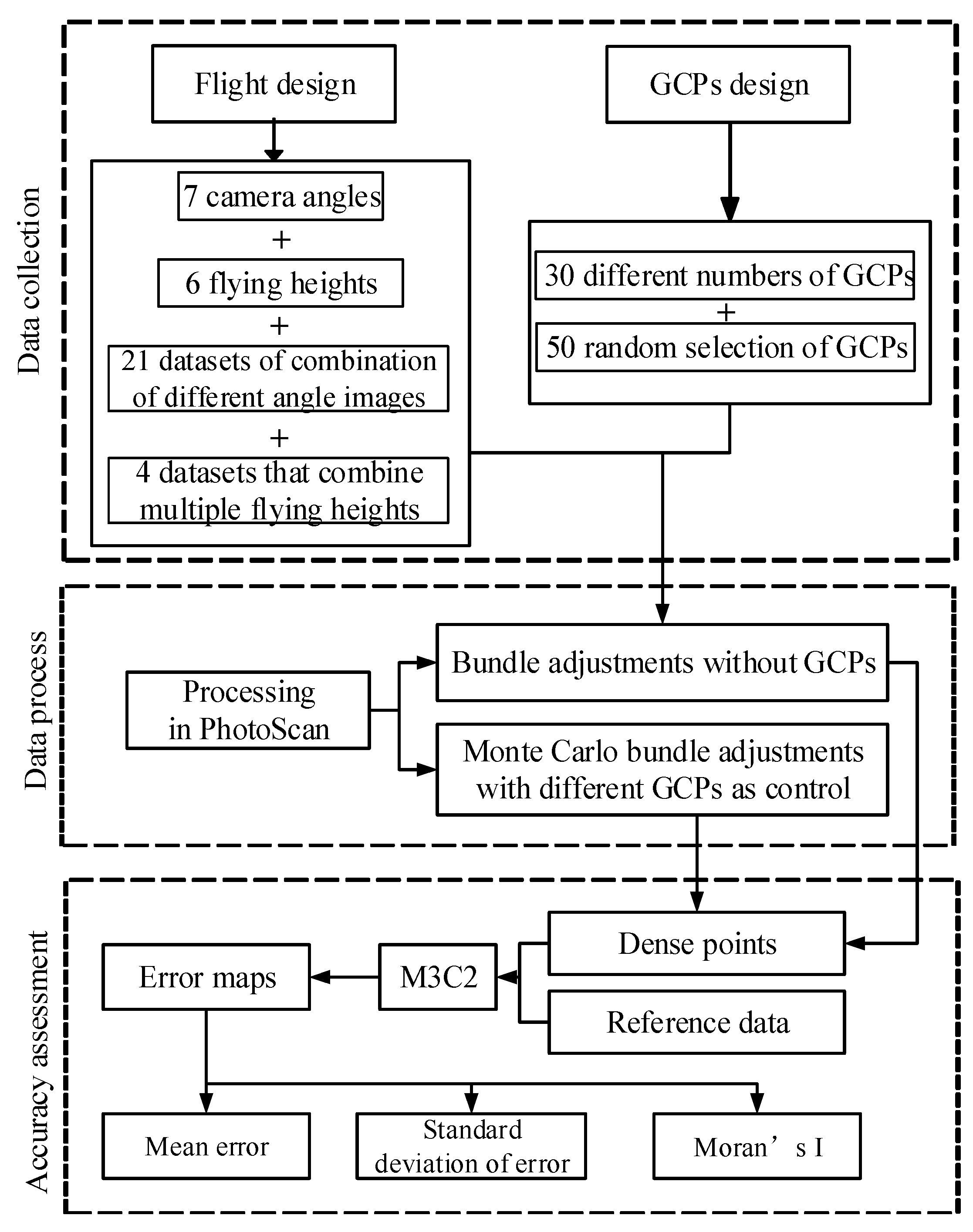
2.1. Overview

To investigate the effects of image collection strategies and GCPs on terrain modeling errors and their spatial structure, we designed different image collection strategies, including 7 various camera angles, 6 different flying heights, and 25 various combination datasets at first (detailed in Section 2.2) in two study areas (Figure 1). Second, the 30 different GCPs and 50 times random selection were used for georeferencing and optimizing the UAV-SfM models (detailed in Section 2.3). Third, more than 105 UAV-SfM scenarios with various combinations of camera angles, flight heights, nadir and/or oblique imagery, and different numbers and distribution of GCPs were processed (2 study areas × (7 camera angles + 6 flying height + 25 various combination datasets) × 30 different numbers of GCPs × 50 random selections of GCPs), and the corresponding point cloud data were generated. Finally, the error maps were generated by comparing the generated point cloud with the reference point cloud. Moreover, the effects of image collection strategies and GCPs on terrain modeling errors were assessed by quantitative analysis of the error maps (mean error, stand deviation error, and Moran’s I).

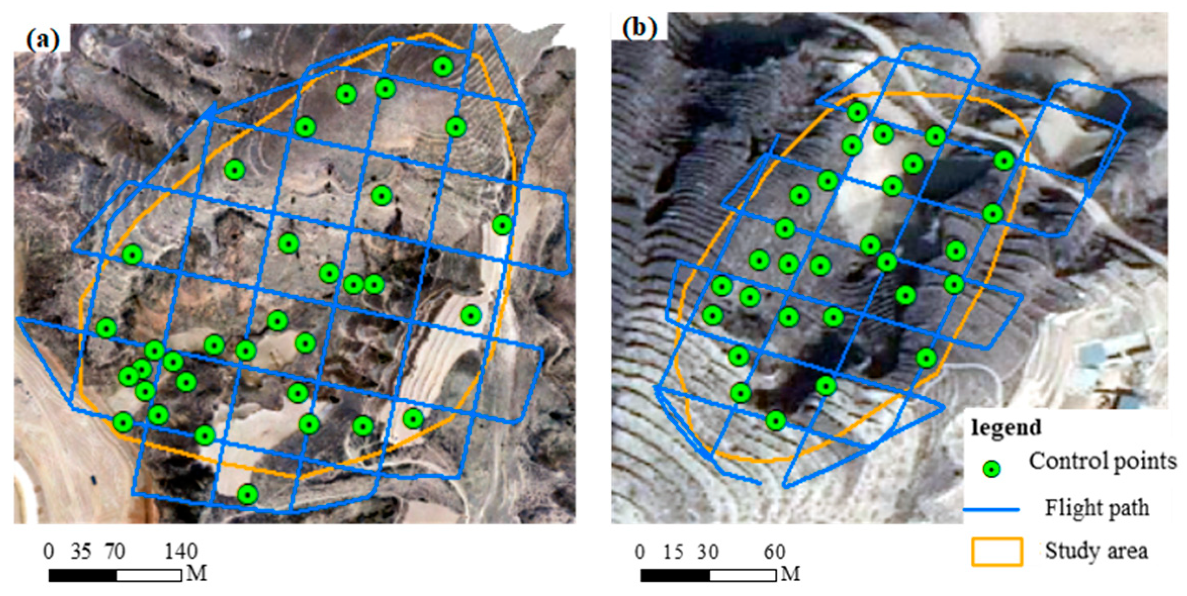
2.2. Image Data Collection

Study Areas

Two small catchments T1 (110°17′3.2″E, 37°33′48.8″N) and T2 (110°21′45.7″E, 37°35′12.8″N) located in Suide county, Shaanxi province, with 5.1 ha (T1) and 3.6 ha (T2), were selected as study areas (Figure 2). The two areas are loess hilly landforms with high relief topography. The maximum height difference is 100 m (T1) and 80 m (T2). We collected the UAV images in the spring of 2021. In this season, the vegetation is sparse, which reduces errors in UAV terrain modeling.

2.3. Image Collection

2.3.1. Camera Angle Design

(1) Single camera with different angles
UAV images were collected using a DJI-Phantom 4 Professional quadcopter equipped standard with a 1″ CMOS camera with 20 megapixels. The on-board GNSS accuracy of this UAV was 1.5 m (horizontal) and 0.5 m (vertical). Due to the low on-board GNSS accuracy, optimizing image collection strategy and ground control quantity is generally needed. The remote-control equipment was used to preset the flight line, overlap, camera inclination, and flying height parameters to control the posture and track of the UAV.
To explore the influence of camera angle on survey errors, the camera angle was varied from 0 to 40° (0° indicating a nadir inclination) within individual surveys. The flight line was designed as a “double-grid” (two orthogonal blocks) grid (Figure 1). During flying, the drone rotates through 180° at the end of each strip, which means that with an angle of 10°, the camera angle is +10° in one line and -10° in the next strip. To minimize the effects of other flight factors, both side and forward overlaps were fixed at 80%, and the flying height remained constant (Table 1). A camera angle bigger than 40° is not included because the observation distance will be much bigger than the flying height under such a high inclination. Due to high-relief landforms, the take-off point was halfway up the mountain, the flying height was set to 100 m (T1) and 70 m (T2), respectively, and the ground resolution was 2.7 cm (T1) and 1.9 cm (T2), respectively (Table 1).
(2) Combination of different camera angles
The combination dataset has been proposed for improving UAV-SfM photogrammetry [36,37]. Here, we designed different combination dataset experiments. We combined a nadir block with supplemented convergent imagery given its importance for reducing systematic error in UAV-SfM photogrammetry [22]. In this study, we added more combinations because an off-nadir double-grid block can also be supplemented with several additional convergent images. Then, we referred to the double-grid blocks (nadir or off-nadir) as the main blocks. The main blocks used were the same as those in Table 1. The additional convergent images with camera angles from 0° to 40° were collected at 120 m and 80 m flying heights in T1 and T2 areas (Table 2), respectively. Each additional convergent dataset comprises 16 photos. The supplemented photos are added into the main block (double-grid blocks), and then all the photos will be regarded as a combination block.

2.3.2. Flying Height Design

(1) Single flying at different heights
Except for the camera angle, the flying height is also an important factor affecting the accuracy. Due to the high relief of the study areas, the actual flying height will be inconstant. Here, we used the average flying height. The flying height directly affects the ground resolution and indirectly affects the elevation accuracy. This study focuses on a 1:500 photography survey. According to Specifications for low-altitude digital aerial photography (CH/Z3005-2010), the ground resolution of 1:500 scale aerial photography should be less than 5 cm. Therefore, we designed a flying height of 60–160 m and the ground resolution is 1.6–4.4 cm (Table 3). For better comparison, we kept the camera angle and the overlap constant under different flying heights. We used a nadir camera for the T1 area and a 15° inclined camera for the T2 area to investigate the effect of camera angle (Table 3).
(2) Combination of multiple flying heights
Here, we combined multiple flying heights into one block because it has also been suggested for improving the UAV-SfM model in previous studies [38]. To investigate whether the number of combined flying heights affects errors or not, we designed the image combinations of 2, 4, and 6 flying heights, and kept the mean flight height the same (Table 4). This experiment can also demonstrate the effect of camera angle on the combinations of flying height because we set a nadir camera and a 15° inclined camera in the T1 and T2 areas, respectively.

2.4. Ground Control Points

2.4.1. Ground Control Design

The GNSS-RTK method is adopted for the field control survey. The GNSS receiver is Topcon HiPer SR, and the size of the control point target is 1 m × 1 m. The horizontal and vertical accuracy for GCPs surveyed with GNSS-RTK were ±0.010 m and ±0.015 m, respectively. The control point (target center) is visible within 200 m flying height. To ensure that the GCPs are evenly distributed on the plane and elevation, we set up GCPs along peaks, ridges, and gully bottoms in each study area. We set up 33 (T1) and 31 (T2) GCPs, respectively, for both study areas (Figure 1) (6.5 and 8.6 GCPs per hectare in T1 and T2 area, respectively).
The UAV data are processed by the 3-D modeling software Agisoft PhotoScan Pro 1.5. The main processing flow includes preliminary processing, aerial triangulation, dense cloud building, point cloud editing, and error spatial distribution map generation. To verify the effect of different image collection strategies on terrain modeling errors, we designed two data processing scenarios: GCP-constrained and GCP-free. With GCP-free scenario, we only used two GCPs to shift, rotate, and zoom the tie points to a correct location for georeferencing; and the two GCPs were excluded from the bundle adjustment process. With GCP-constrained scenario, GCPs were used to improve the bundle adjustment. Here, two factors need to be considered, including the number and the spatial distribution of GCPs.

2.4.2. The Number of GCPs

To investigate the effect of the number of GCPs and whether different image collection strategies affect the optimal GCP number, we employed two Monte Carlo GCP experiments [29] under different image collection strategies. First, for each Monte Carlo realization, the same number (x) of GCPs was selected to optimize the bundle adjustment, and the rest of the GCPs were used as check points to assess the accuracy. The process was then repeated 50 times with a different random selection of GCPs. Second, for each Monte Carlo realization, the number of selected GCPs gradually increased from 10% to 90% of the total GCPs (33 and 31 for the T1 and T2 area, respectively) in steps of 10%. The Monte Carlo GCP tests were carried out in the Agisoft PhotoScan Pro 1.5 and using the Python code [29].

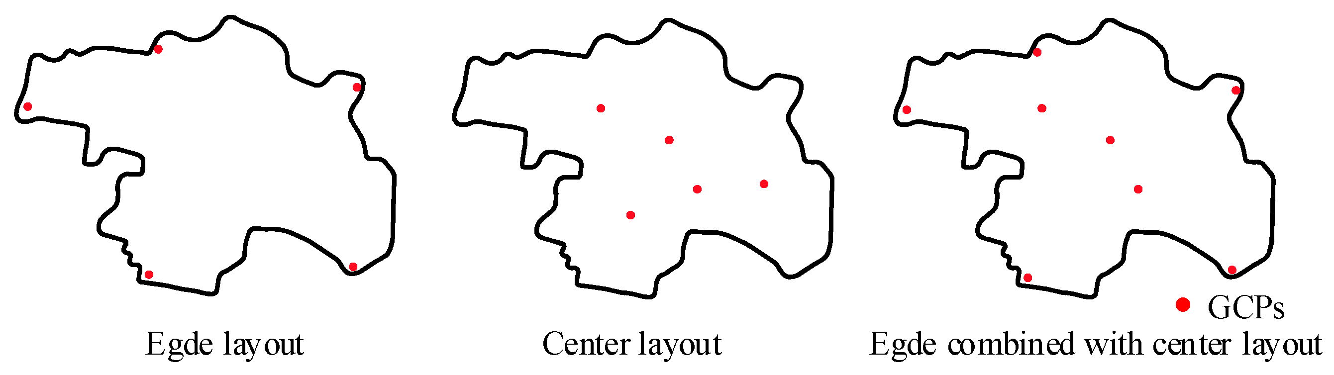
2.4.3. The Spatial Distribution of GCPs

To investigate the effect of the spatial distribution of GCPs, we used two indices for quantifying the spatial pattern of GCPs. The mean distance between GCPs (MEDCP) is the sum of the distance between GCP pairs divided by the number of GCP pairs, which can reveal whether the GCPs are evenly distributed in space:
MEDCP = 1 n d i n
where, the di is the distance of a GCP pair; n is the number of GCP pairs.
The Compaction Index (CI) of GCPs is the ratio of the perimeter of the convex hull of GCPs to the square root of the convex hull area of GCPs, which shows the shape of the GCP distribution:
CI = P A
where, the p is the perimeter of the convex hull of GCPs; A is convex hull area of GCPs. The smaller the value of CI, the closer the shape of the convex hull area is to a circle, indicating that it is less compact. The bigger the value of CI, the closer the shape of the convex hull area is to a straight line, indicating that it is more compact.
Besides the two indices to quantify the spatial pattern of GCPs, three patterns that edge layout, center layout, and edge combined with center layout (Figure 3) are used to validate the effect of the indices due to the obvious differences of the three layouts in the indices. Among the three layouts, the MEDCP of edge layout is the largest, followed by the edge combined with center layout, and the center layout. With a same layout (e.g., center layout), the CI varies with the GCP distribution. A larger CI can represent the discrete distribution of the convex hull of GCPs.

2.5. Accuracy Evaluation

We used all the GCPs (33 GCPs for T1 and 31 GCPs for T2) for georeferencing and controlling the photogrammetry process to generate the reference data. Due to the high density of GCPs in the two areas, the reference data generated by all GCP control have a high accuracy. This study focuses on the error of terrain elevation (Z error). We used the M3C2 tool in CloudCompare to evaluate the elevation error of each point between the experimental results (generated by the different experimental methods in Section 2.3 and Section 2.4) and the reference data. The evaluated elevation error point cloud is then converted to a raster to obtain the error maps. Thereafter, we used the standard deviation error (STD) and mean error (ME) of the error map to represent the overall error of the study areas. ME reflects the overall systematic error. A large ME shows a systematic error in the study area. STD reflects the level of random error, and the smaller the STD, the smaller the random error. The two calculation formulas are shown below:
S T D = i = 1 n ( x i x ¯ ) 2 n
M E = i = 1 n x i n
where n represents the number of pixels; x i represents each elevation error in each pixel; and x ¯ represents the average error.
In addition, this study calculates Moran’s I [39] to quantify the autocorrelation of the error maps because ME and STD do not consider the extent to which error is spatially variable. The Moran’s I reflects the spatial structure (clustering or discrete) of errors. If the errors present a clustering or discrete pattern, there is a systematic error. Thus, Moran’s I is important for revealing systematic error. The value of Moran’s I is between −1 and 1: The closer its value to 1 or −1, the more positive or negative the spatial autocorrelation of errors, respectively. A value of 0 indicates a random distribution of error in space:
I = n S o · i = 1 n j = 1 n w i , j ( x i x ¯ ) ( x j x ¯ ) i = 1 n ( x i x ¯ ) 2
where n is the number of spatial units indexed by i and j ; x is the variable of interest; x ¯ is the mean of x ; w i , j is a matrix of spatial weights with zeroes on the diagonal; and S o is the sum of all w i , j .

3. Results

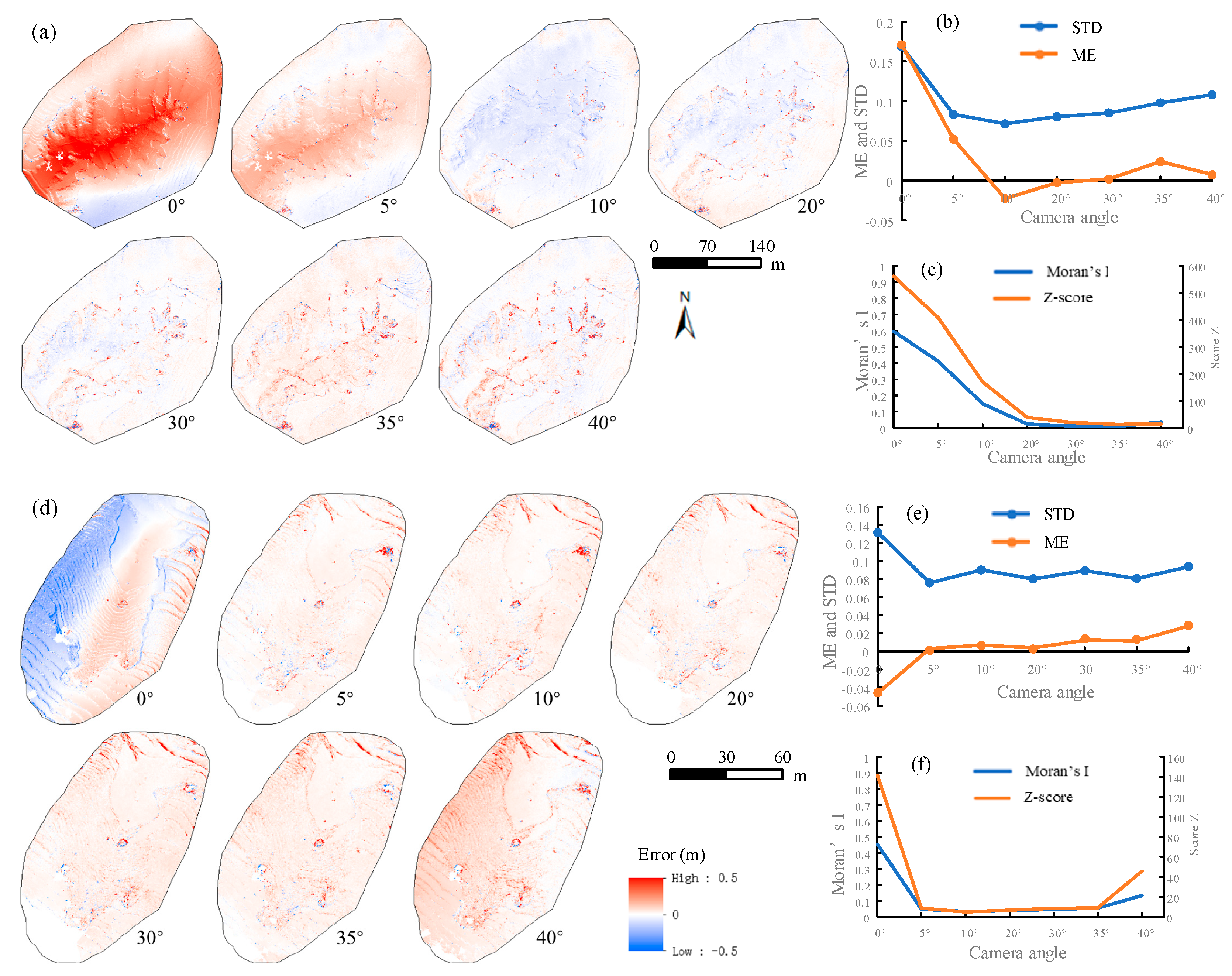
3.1. The Effects of Camera Angle

3.1.1. Single Camera Angle

The error maps with different camera angles are shown in Figure 4. Errors in T1 and T2 areas show the same spatial distribution pattern. When the camera angle is 0°, the error map shows an obvious spatial clustering pattern. Positive errors are concentrated in the valley area, and negative errors are concentrated in the ridge area. When the camera angle is greater than or equal to 10°, the spatial distribution of errors are relatively even. Then, we use ME and STD to quantify the overall accuracy of the study areas. When the camera angle is 0°, the ME of the two areas is the largest; when the camera angle is greater than 10°, the ME is close to 0, indicating that the georeferencing in Z direction is acceptable. The trend of the STD is the same as the ME, indicating that the use of oblique photography reduces the magnitude of errors. However, the STD is larger than ME with a higher camera angle (>20°) (Figure 4b,e), indicating that the systematic error is optimized and then the random error dominates.
The Moran’s I reveals that the structure of errors varies with camera angle. The Moran’s I is positive with nadir and 5° camera angle in the two study areas (Figure 4c,f) (P values are less than 0.01, and Z values are greater than 1.96), showing that the spatial distribution of errors has positive spatial correlation, that is, the errors are clustered in space; this is consistent with the error maps in Figure 4a,d. As the camera angle increases, Moran’s I decreases rapidly. After the camera angle is greater than 10°, Moran’s I gradually stabilizes and closes to 0, indicating that the error is similar to the spatial random distribution. This result means that using oblique photography with a large camera angle (greater than 20°) not only reduces the magnitude of errors but also improves the spatial structure of errors.

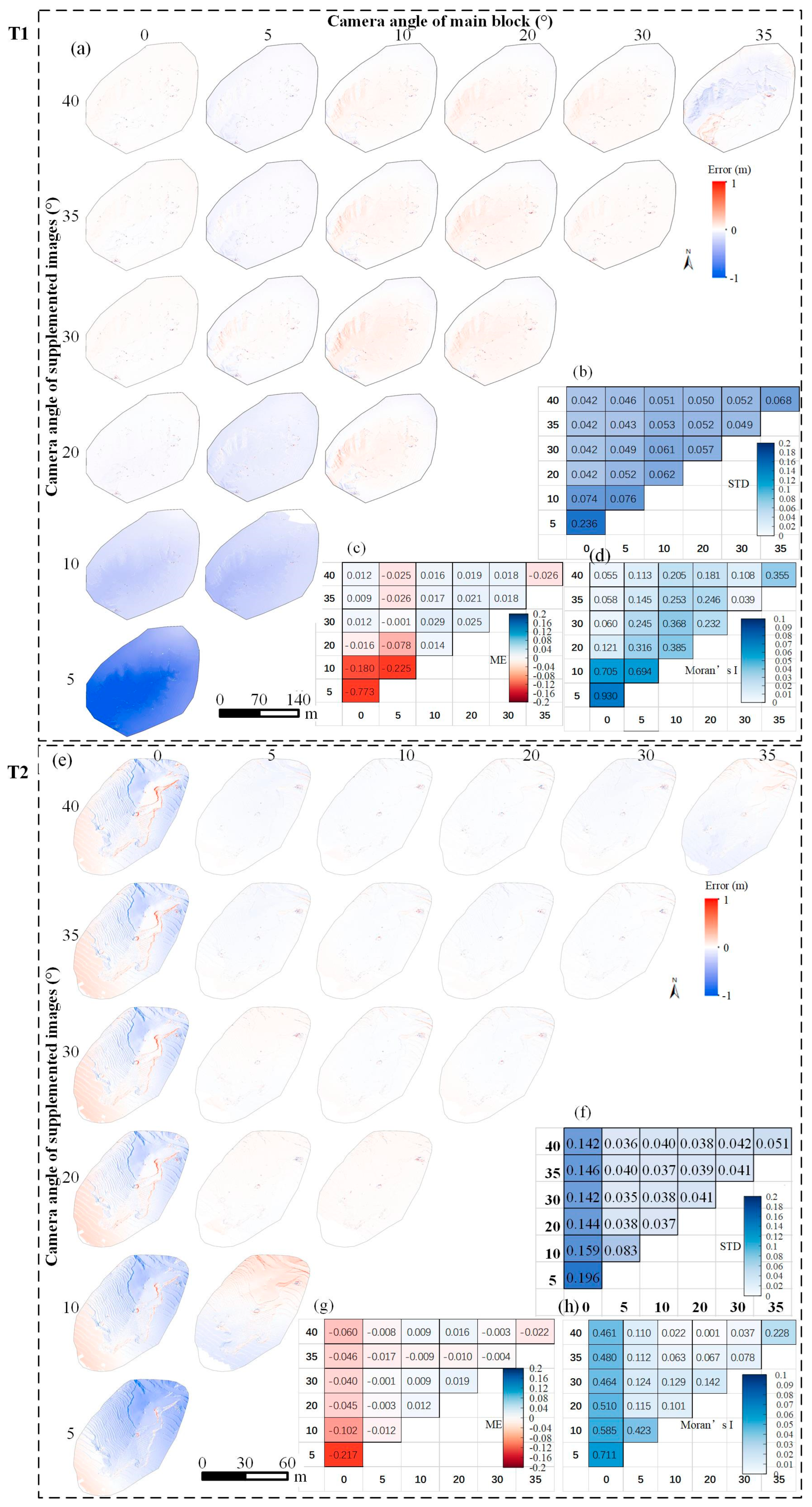
3.1.2. Combination of Different Camera Angles

Figure 5 shows the error maps with different combinations of camera angles. When both the main block angle and supplemented image angle are low (0° or 5°), the errors show a spatial clustering pattern, and a bigger ME, STD, and Moran’s I. With an increasing supplemented image angle, the spatial distribution of errors can improve, which is supported by a reduced ME, STD, and Moran’s I. However, when the main block angle is higher than 10°, supplementing with additional oblique images seems to have no effect on the error patterns. This means that if the main block has a relatively high camera angle, the supplemented convergent images are unnecessary.

3.2. The Effects of Flying Height

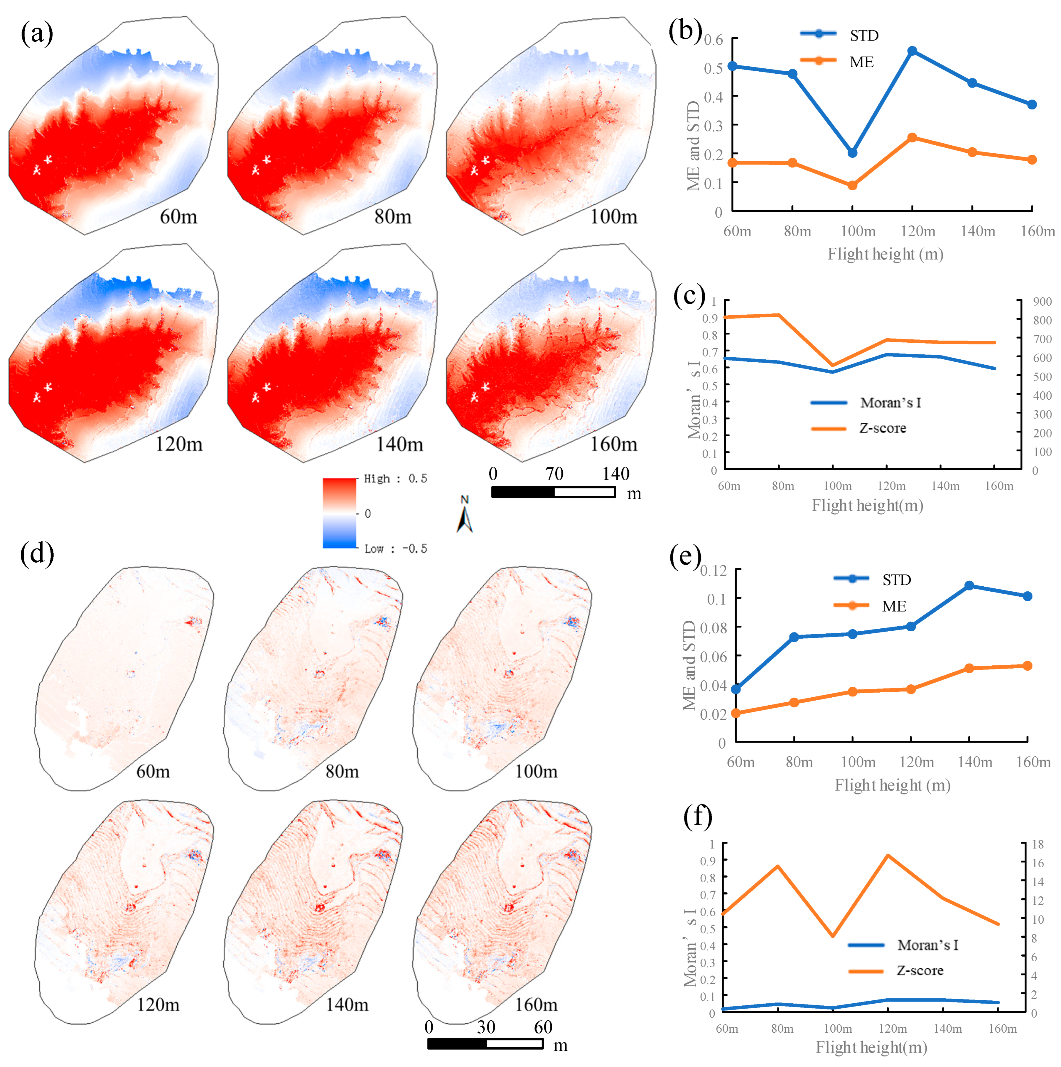
3.2.1. Single Flying Height

Figure 6 shows the error maps with different flying heights. The T1 area presents stable ME and STD values with increasing flying height with a nadir (0°) camera; while the ME and STD increase in the T2 area where a 15° camera angle was used. Generally, the ME and STD would increase with flying height due to an increase in observation distance and coarser image resolution. The T1 area shows an unexpected result. This could be due to two reasons. First, the error is decimeter level with the nadir camera (supported by Figure 4d,e). The error changes caused by flying height (60–160 m only) could be an order lower than the error caused by the nadir camera. The photogrammetric solutions were still dominated by camera calibration effects, not flying height. Thus, the experimental results cannot reflect the error variation caused by flying height. This conclusion is supported by the results from the T2 area. In the T2 area, there is a significant positive correlation between the flying height, ME, and STD since the T2 area adopts oblique photography with a camera angle of 15° and the error is centimeter-level which is enough to capture the change caused by flying height.
Figure 6 also confirmed the conclusion in Section 3.1 that oblique photography with a large angle reduces the elevation error in high-relief landforms, and its error spatial distribution is more even. However, the flying height marginally affects the spatial patterns of errors. Although the flying height is changing (60–160 m), the spatial distribution of errors shows the same pattern (Figure 6a,d). The Moran’s I slightly increases with the flying height (Figure 6c,f). By contrast, the camera angle is more important than flying height for improving the spatial pattern of errors. The Moran’s I in the T1 area with oblique photography is an order of magnitude less than that in the T2 area with vertical photography.

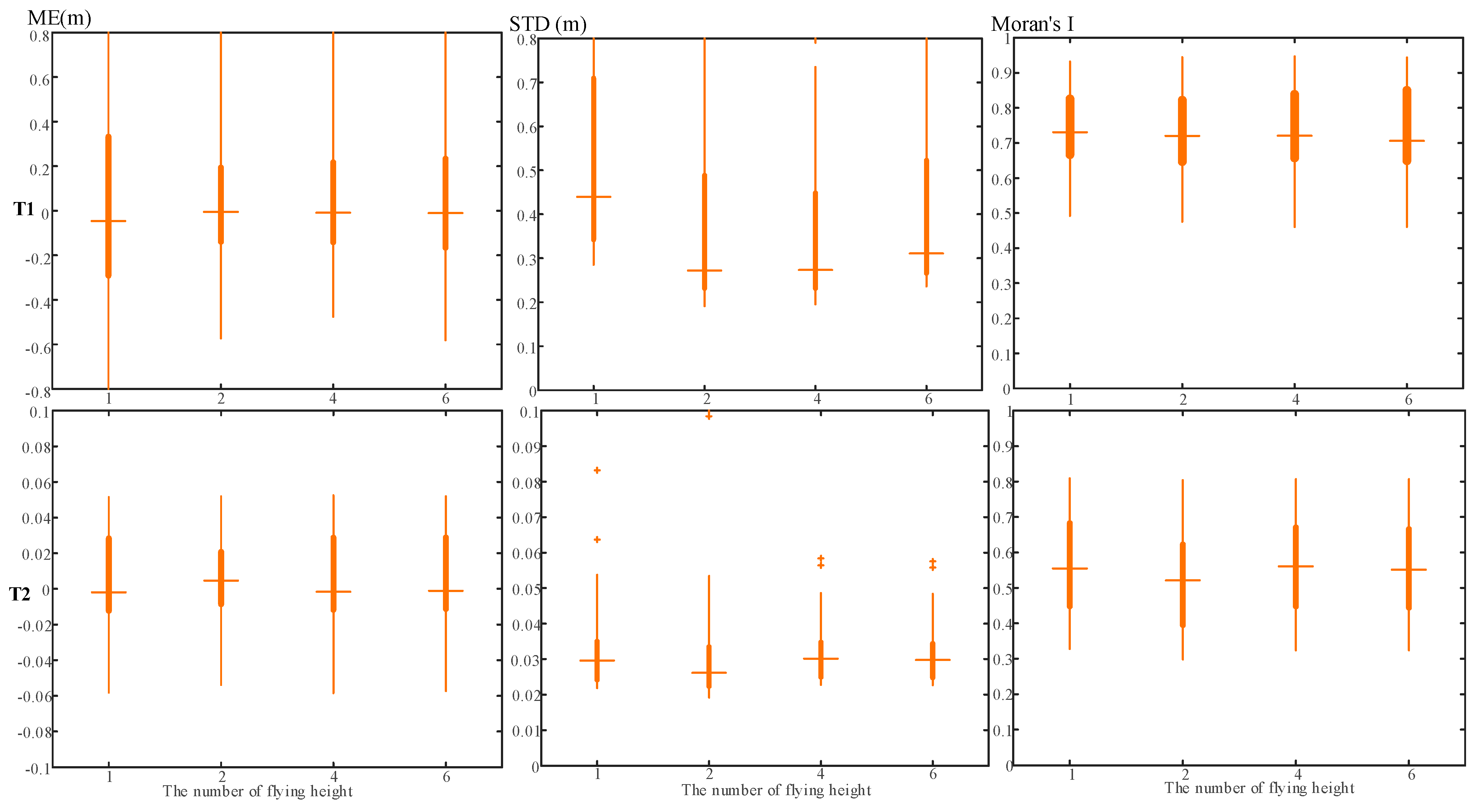
3.2.2. Combination of Multiple Flying Heights

Figure 7 shows the effects of different combinations of flying heights on ME, STD, and Moran’s I. The combined multiple flying heights do not impact ME and Moran’s I, but they do affect STD. In the T1 area, where the nadir camera is utilized, increasing the flying heights from one to two exhibits a decreasing trend in STD. This implies that additional observation distance enhances accuracy. Conversely, the flying height appears to have no effect on the STD of the T2 area. The disparity between T1 and T2 can be attributed to the fact that in T2 all flights are conducted with a 15° camera angle, resulting in variable observation distances within the image. As a result, incorporating additional flying height does not yield a discernible difference in oblique photogrammetry. The additional flying height is unnecessary when using oblique photography.

3.3. The Effects of GCPs

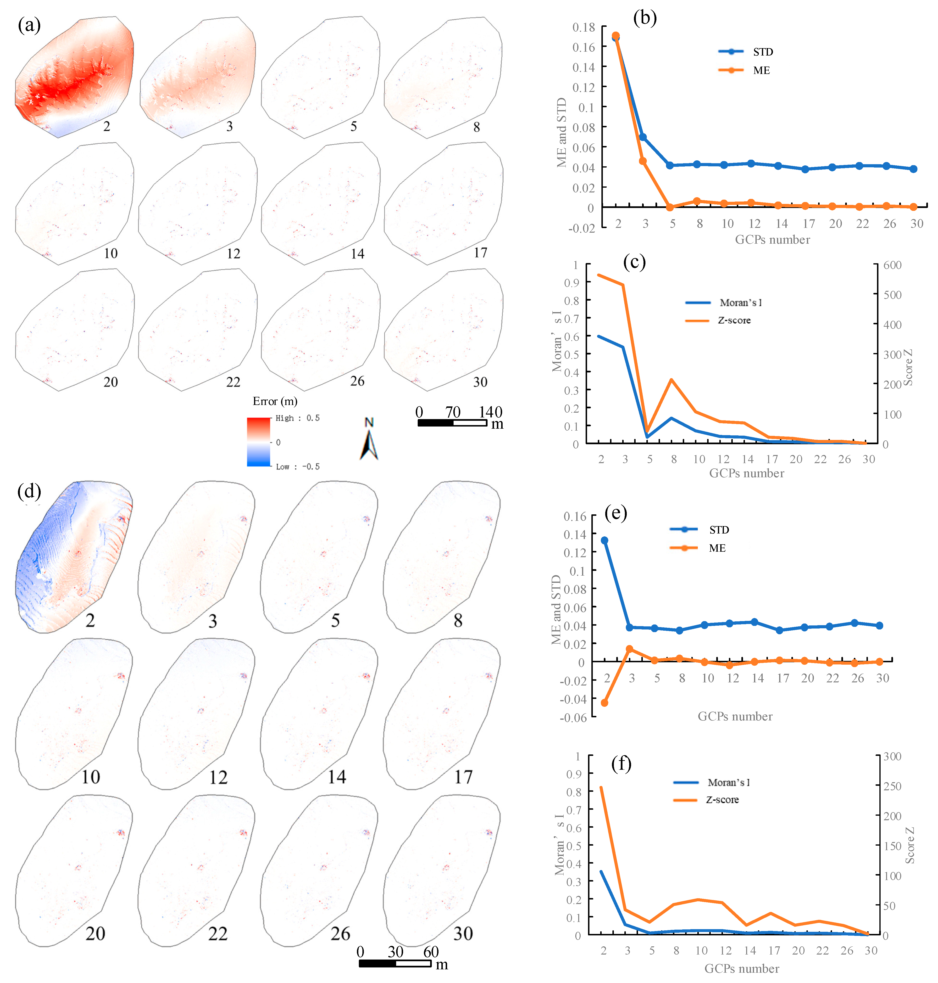
3.3.1. The Number of GCPs

Figure 8 shows the error maps with different numbers of GCPs. The overall trends of the T1 and T2 areas are similar. As the number of GCPs increases, the magnitude (ME and STD) of the error becomes smaller, and its spatial distribution is also improved, similar to the random distribution (Figure 8a,b). The STD and ME of the two areas are negatively correlated with the number of GCPs (Figure 8c,d). However, when the GCPs reach a certain number (about 5 GCPs), the STD and ME tend to be stable. This means that a small number of GCPs can rapidly improve the overall accuracy of the area, but after reaching a certain number, the GCPs have minor influence on the magnitude of the errors.
We calculated Moran’s I of the errors under different numbers of GCPs (Figure 8c,f) for quantifying the spatial structure of errors. When the number of GCPs is small, Moran’s I is relatively large; this indicates a positive spatial correlation of the spatial distribution of errors, and there are high- and low-value clustering distributions in space. However, Moran’s I is negatively correlated with the number of GCPs overall. The more the GCPs, the closer Moran’s I is to 0. After the GCPs exceed a certain number (15 GCPs in the T1 area and 12 GCPs in the T2 area), the Moran’s I becomes stable. The stable number of GCPs for Moran’s I is greater than that of ME and STD (about five GCPs in Figure 8). This implies that a small number of GCPs can rapidly improve the magnitude of the errors and reach a certain level of stability; but, more GCPs are needed for optimizing the spatial structure of errors.

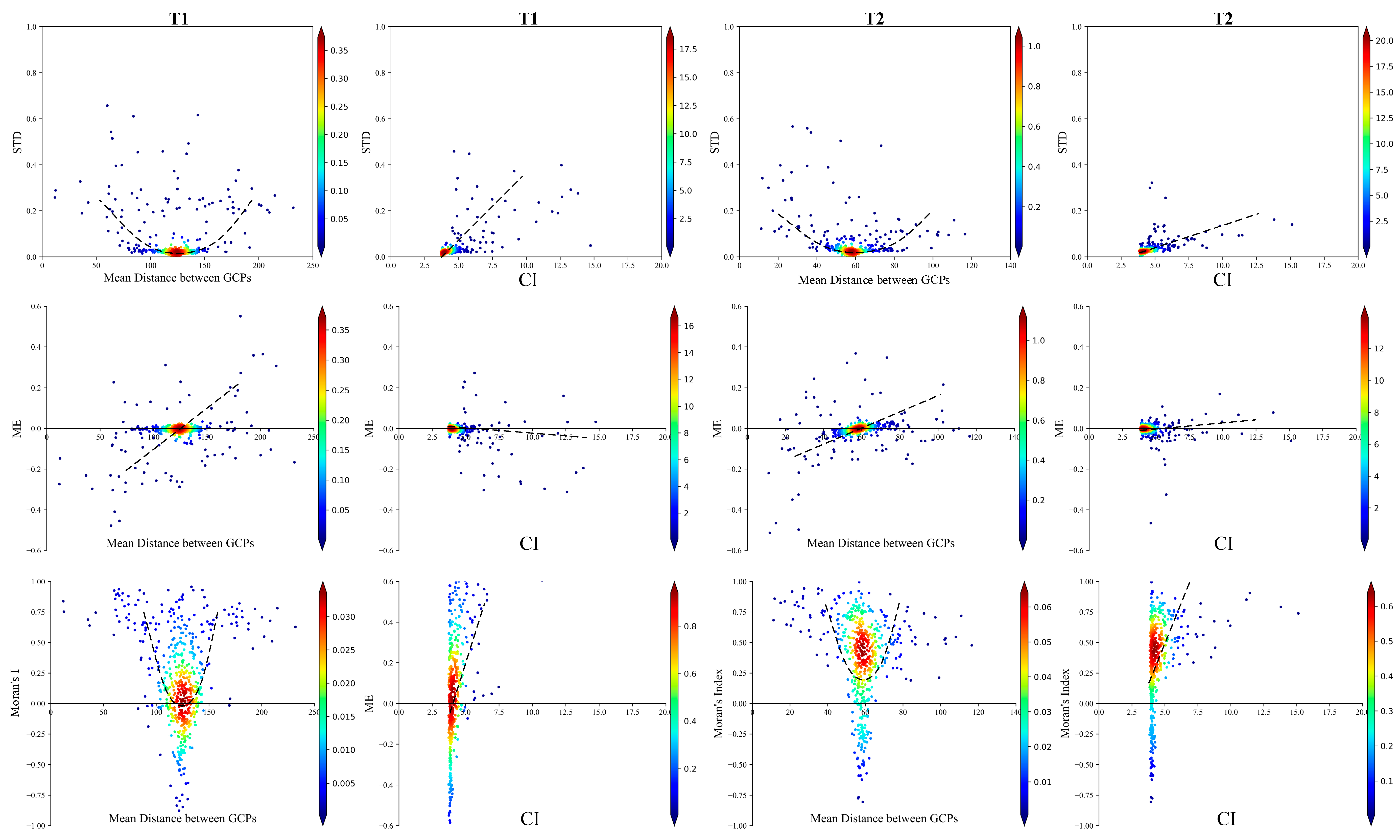
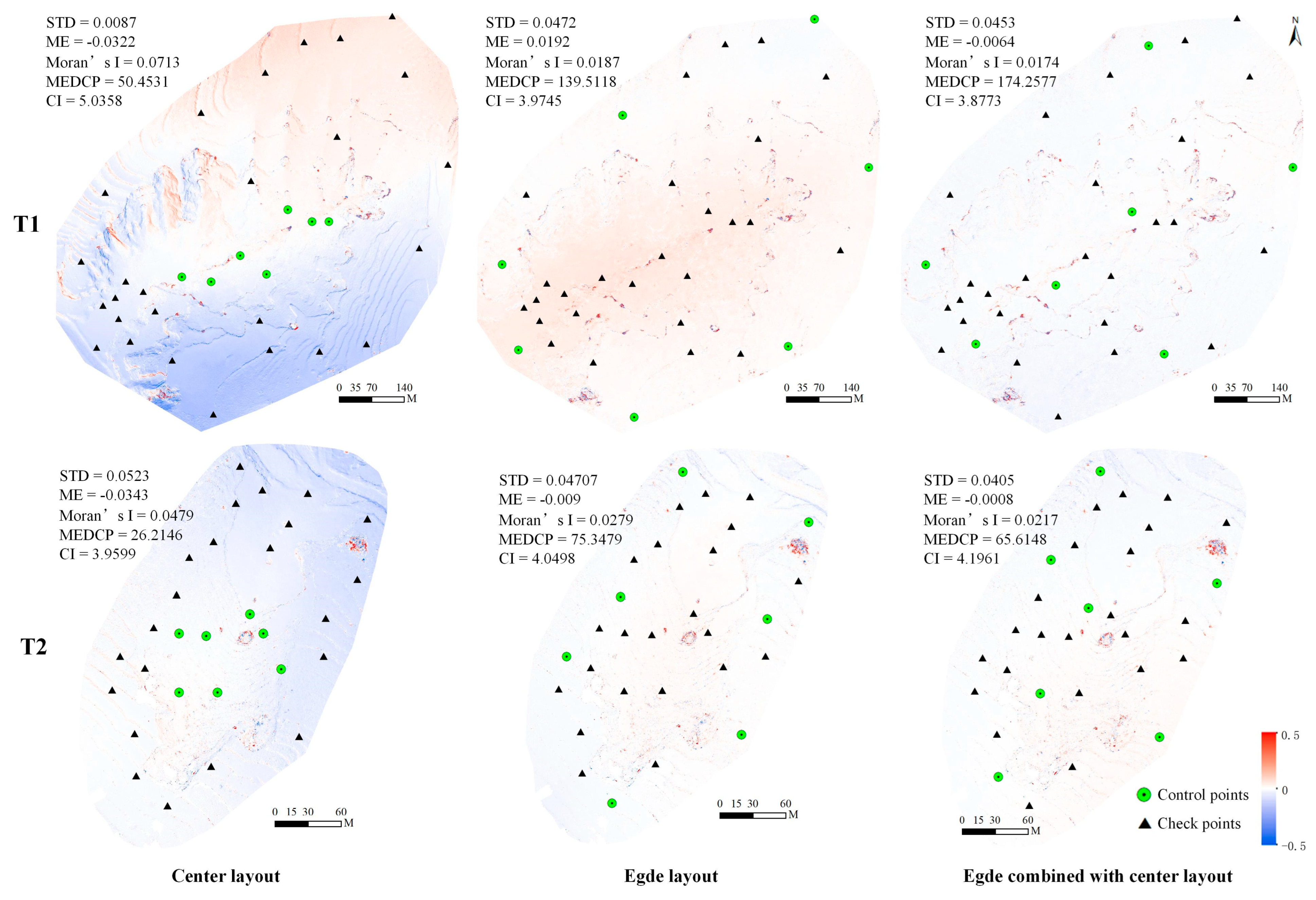
3.3.2. The Spatial Distribution of GCPs

Figure 9 shows the effect of the spatial distribution of GCPs on ME, STD, and Moran’s I. The two study areas show the same trend. The closer the MEDCP is to the average distance of the study areas (about 125 m and 60 m for the T1 and T2 area, respectively), the smaller the STD is, and the closer to zero ME and Moran’s I are. This means that the even distribution of GCPs is better for improving both the magnitude and spatial structure of errors. Meanwhile, the results of CI show that the closer the convex hull area of GCPs is to a circle, the smaller the ME, STD, and Moran’s I. This implies that GCPs should be discretely distributed at the edge of the study area as much as possible, which could be more important than even distribution.
To validate the findings in Figure 9, the edge layout, center layout, and edge combined with the center layout are used to reveal the error maps with different GCP distributions. Figure 10 shows the error maps of the three layouts of GCPs. With the center layout, the MEDCP is the smallest among the three layouts. Obvious spatial autocorrelation exists in the error maps regardless of high or low CI value, indicating systematic errors to some extent. With the edge layout, the MEDCP is the largest among the three layouts. The spatial autocorrelation (Moran’s I) is reduced but still exists, especially in the central area. For the edge combined with the center layout, the MEDCP is the median among the three layouts. The spatial autocorrelation is optimized as much as possible; the ME, STD, and Moran’s I are the lowest. Notably, compared with the edge layout, the edge combined with the center layout only has a slight improvement although more GCPs were used; this suggests that the discrete distribution at the edge of the study area is more important than the even distribution of the whole area.

4. Discussion

4.1. Camera Angle, Flying Height, and Combination Strategies

This study estimated error maps of UAV-SfM photogrammetry. We provide more insights into image collection strategies than traditional overall accuracy indexes, such as RMSE. Previous studies have confirmed that oblique photography with a larger angle can effectively reduce elevation error [24,25]. The experimental results presented in this paper support this finding. Furthermore, we discovered that oblique photography with larger angles improves the spatial distribution of errors. The improvement achieved through higher camera inclination can be attributed to the increased intersection angles of tie point rays, which enhance bundle adjustment, leading to improved camera calibration and error mitigation.
Theoretically, as the flying height increases, the ground resolution becomes coarser and increases errors [40]. A previous study showed the effect of flight altitude on topographic accuracy is nonlinear [3]. Our study also supported this finding. We found that the effect of flying height is relative to camera angle, which means there could be an interactive effect of camera angle, flying height, and other image collection strategies. With oblique photography, the errors decrease by an order of magnitude and the effect of the flying height variation on errors is obvious (Figure 6). Whilst, with vertical photography, the error is relatively large and the flying height seems to have no effect on errors (Figure 6). Then, a possible reason is that error is still dominated by camera calibration effects and not flying height, and the error caused by flying height variation could not be reflected. Moreover, we found that the flying height marginally affected the spatial pattern of errors (Figure 6a,d). By contrast, the camera angle is more important than flying height for improving the spatial pattern of errors (Figure 6c,f).
A combination of datasets was proposed for improving UAV-SfM photogrammetry in previous studies [24,38]. Our study shows that such combinations of datasets may not be necessary if the main block has imageries with a relatively high inclination. Thus, compared to the camera angle, the supplemented convergent images and combined multiple flying height images seem to be unimportant although extra effort has been made.

4.2. The Quantity and Spatial Distribution of GCPs

The quantity and spatial distribution of GCPs is important to improve UAV photogrammetry. GCPs define the absolute orientation and scale of the external coordinate system and provide constraints for the bundle adjustment [24,29,38,41]. Our results show that a small number of GCPs can rapidly improve photogrammetric errors. After more than 5 GCPs, the magnitude of errors tends to be stable, which means a large number of GCPs is unnecessary. However, the spatial structure of errors can be further improved although the magnitude of GCPs is stable. Relatively, more GCPs are required to optimize the spatial structure of errors.
In the two study areas, a range of five to nine GCPs (equivalent to 1.39 to 1.76 GCPs per hectare) is sufficient for improving the bundle adjustment. The appropriate number of GCPs may be influenced by the size of the study sites. In this study, since the study area was relatively small (3.6 to 5.1 hectares), fewer GCPs were required. However, the study [27] reported that a study area of 1220 hectares necessitated 50 GCPs (approximately 0.041 GCPs per hectare). Thus, the average GCP density is more useful than the optimal GCP number in practice. Furthermore, the average GCP density varies across different studies [22,42], indicating that it is dependent on various factors, such as terrain relief, surface texture, and image quality. Hence, there is no universal recommendation for the average GCP density or the optimal number of GCPs in different areas.
In addition to the number of GCPs, the spatial distribution of GCPs should be addressed [27,29]. With the fixed number of GCPs, the different selections of GCPs have different ME, STD, and Moran’s I (Figure 10). There is a general consensus that GCPs should be evenly distributed in study areas [27,29,43]. Our results confirmed this rule. However, we argue that the edge distribution is more important than the even distribution. With a limited or small number of GCPs, we should first discretely distribute GCPs at the edge of study areas as much as possible, and then even distribution could be considered.

4.3. Other Factors

In addition to the image collection and ground control strategies, the terrain relief seems to be another variable that influences UAV-SfM photogrammetry accuracy. Previous studies [3,10,11,12] investigated different UAV-SfM strategies in plain and forest areas. In this study, we focused on two hilly areas. UAV-SfM in hilly areas have more inconstant ground resolution and terrain shadings, and thus suitable image collection and ground control design are needed. However, the study [22] also showed that terrain modeling errors in low-relief regions can be complex due to the fewer variations in UAV observation distance. The image collection and ground control strategies presented in this paper can also be applied to low-relief (plain) regions because oblique photography can increase the variation in UAV observation distance and enhance bundle adjustment.
The different flight configurations (image collection and ground control strategies) affect the critical steps of the SfM algorithm, such as key point extraction, feature matching and dense matching, and finally their effects are reflected in accuracy. First, oblique images capture steep slopes that are often not visible in nadir images [44], resulting in a greater number of potential matching points in both the SfM and MVS processes. This finding aligns with the results of [24], who reported that oblique images enhance tie-point matching. Moreover, higher camera inclination can increase intersection angles of tie point rays, which enhance bundle adjustment, leading to improved camera calibration. Second, lower flying altitude increased the image quality. The high-quality images lengthen the processing time because of the smaller pixel size and larger number of pixels. Besides the processing time, the larger number of pixels provides potentiality to extract more key points and then enhance feature matching in the SfM algorithm. Finally, the interactions of camera angle, flying height, GCPs, and terrain relief can be complex. For example, oblique photography increases the variation of observation distance and the intersection angles of tie point rays, which is beneficial for bundle adjustment; but the perspective deformations of oblique photography may introduce more false key point matches in flats with a similar repetition of textures [45], leading to an unpredictable result. Thus, the mechanism of interactions of these factors is still unknown and needs to be investigated in the future.

5. Conclusions

From the perspective of spatial structure of errors, this study designed various UAV-SfM photogrammetric scenarios and investigated the effects of image collection strategies (camera inclination, flying height, and combination dataset) and GCPs (the number and distribution) on terrain modeling. The error maps of different photogrammetric scenarios were calculated. Then, the error maps were quantitatively analyzed by ME, STD, and Moran’s I. The results show that:
  • A high camera inclination (20–40°) enhances UAV-SfM photogrammetry. This not only decreases the magnitude of errors, but also mitigates its spatial correlation (Moran’s I). Supplementing convergent images is valuable for reducing errors in a nadir camera block, but it is unnecessary when the image block is with a high camera angle.
  • Flying height increases the magnitude of errors (ME and STD) but does not affect the spatial structure (Moran’s I). By contrast, the camera angle is more important than flying height for improving spatial pattern of errors. Moreover, the effect of flying height is nonlinear and could interact with the camera angle.
  • A small number of GCPs rapidly improves the magnitude of errors (ME and STD), and a further increase in GCPs has a marginal effect. However, the structure of errors (Moran’s I) can be further improved with increasing GCPs.
  • With the same number, the distribution of GCPs is critical for UAV-SfM photogrammetry. The edge distribution should be first considered, followed by the even distribution.
UAV-SfM photogrammetry is easily accessible for producing high-resolution (centimeter-level) orthoimages and digital elevation models at low cost and is thus widely used in geoscience communities. The “best practice” of UAV-SfM photogrammetry is arousing wide concern in research communities. This study recommended photogrammetric guidelines based on robust analyses of camera settings and GCPs design. The research findings contribute to understanding how different image collection scenarios (camera inclination and altitude) and ground control points can influence subsequent terrain modeling accuracy and precision (ME and STD). Besides accuracy and precision, this study used a spatial autocorrelation statistic (Moran’s I) for determining the extent of spatial structure of errors. The results show that the spatial dependence statistic of error like Moran’s I should be routinely applied in evaluations of the quality of UAV-SfM photogrammetry.

Author Contributions

Conceptualization, W.D. and B.W.; methodology, W.D.; software, W.L.; validation, R.Q., G.Z. and W.L.; resources, G.W.; writing—original draft preparation, W.D.; writing—review and editing, R.Q., S.O.Y.A. and W.L.; supervision, B.W. and G.W.; project administration, W.D.; funding acquisition, W.D. and G.W. All authors have read and agreed to the published version of the manuscript.

Funding

We are grateful for the financial support provided by the National Natural Science Foundation of China (No. 42301478, 42371060, and 42275028), the Natural Science Foundation of the Jiangsu Higher Education Institutions of China (No. 22KJB170016).

Data Availability Statement

The data that support the findings of this research are available from the author upon reasonable request.

Acknowledgments

Many thanks are given to Guanghui Hu, Xiaoli Huang, Yue Li, and Ling Yang for their assistance in data collection.

Conflicts of Interest

The authors declare no conflict of interest.

References

  1. Shahbazi, M.; Menard, P.; Sohn, G.; Theau, J. Unmanned aerial image dataset: Ready for 3D reconstruction. Data Brief 2019, 25, 103962. [Google Scholar] [CrossRef] [PubMed]
  2. Pierzchała, M.; Talbot, B.; Astrup, R. Estimating Soil Displacement from Timber Extraction Trails in Steep Terrain: Application of an Unmanned Aircraft for 3D Modelling. Forests 2014, 5, 1212–1223. [Google Scholar] [CrossRef]
  3. Chen, C.; Tian, B.; Wu, W.; Duan, Y.; Zhou, Y.; Zhang, C. UAV photogrammetry in intertidal mudflats: Accuracy, efficiency, and potential for integration with satellite imagery. Remote Sens. 2023, 15, 1814. [Google Scholar] [CrossRef]
  4. Gonçalves, J.A.; Henriques, R. UAV photogrammetry for topographic monitoring of coastal areas. ISPRS J. Photogramm. Remote Sens. 2015, 104, 101–111. [Google Scholar] [CrossRef]
  5. Jaud, M.; Bertin, S.; Beauverger, M.; Augereau, E.; Delacourt, C. RTK GNSS-Assisted Terrestrial SfM Photogrammetry without GCP: Application to Coastal Morphodynamics Monitoring. Remote Sens. 2020, 12, 1889. [Google Scholar] [CrossRef]
  6. Manfreda, S.; McCabe, M.; Miller, P.; Lucas, R.; Pajuelo Madrigal, V.; Mallinis, G.; Ben Dor, E.; Helman, D.; Estes, L.; Ciraolo, G.; et al. On the Use of Unmanned Aerial Systems for Environmental Monitoring. Remote Sens. 2018, 10, 641. [Google Scholar] [CrossRef]
  7. Cao, L.; Liu, H.; Fu, X.; Zhang, Z.; Shen, X.; Ruan, H. Comparison of UAV LiDAR and Digital Aerial Photogrammetry Point Clouds for Estimating Forest Structural Attributes in Subtropical Planted Forests. Forests 2019, 10, 145. [Google Scholar] [CrossRef]
  8. Candiago, S.; Remondino, F.; De Giglio, M.; Dubbini, M.; Gattelli, M. Evaluating Multispectral Images and Vegetation Indices for Precision Farming Applications from UAV Images. Remote Sens. 2015, 7, 4026–4047. [Google Scholar] [CrossRef]
  9. Bendig, J.; Yu, K.; Aasen, H.; Bolten, A.; Bennertz, S.; Broscheit, J.; Gnyp, M.L.; Bareth, G. Combining UAV-based plant height from crop surface models, visible, and near infrared vegetation indices for biomass monitoring in barley. Int. J. Appl. Earth Obs. Geoinf. 2015, 39, 79–87. [Google Scholar] [CrossRef]
  10. Tu, Y.-H.; Phinn, S.; Johansen, K.; Robson, A.; Wu, D. Optimising drone flight planning for measuring horticultural tree crop structure. ISPRS J. Photogramm. Remote Sens. 2020, 160, 83–96. [Google Scholar] [CrossRef]
  11. Swayze, N.C.; Tinkham, W.T.; Vogeler, J.C.; Hudak, A.T. Influence of flight parameters on UAS-based monitoring of tree height, diameter, and density. Remote Sens. Environ. 2021, 263, 112540. [Google Scholar] [CrossRef]
  12. Kameyama, S.; Sugiura, K. Effects of differences in structure from motion software on image processing of unmanned aerial vehicle photography and estimation of crown area and tree height in forests. Remote Sens. 2021, 13, 626. [Google Scholar] [CrossRef]
  13. Zhao, N.; Lu, W.; Sheng, M.; Chen, Y.; Tang, J.; Yu, F.R.; Wong, K.-K. UAV-Assisted Emergency Networks in Disasters. IEEE Wirel. Commun. 2019, 26, 45–51. [Google Scholar] [CrossRef]
  14. Erdelj, M.; Natalizio, E.; Chowdhury, K.R.; Akyildiz, I.F. Help from the Sky: Leveraging UAVs for Disaster Management. IEEE Pervasive Comput. 2017, 16, 24–32. [Google Scholar] [CrossRef]
  15. Tuna, G.; Nefzi, B.; Conte, G. Unmanned aerial vehicle-aided communications system for disaster recovery. J. Netw. Comput. Appl. 2014, 41, 27–36. [Google Scholar] [CrossRef]
  16. Westoby, M.J.; Brasington, J.; Glasser, N.F.; Hambrey, M.J.; Reynolds, J.M. ‘Structure-from-Motion’ photogrammetry: A low-cost, effective tool for geoscience applications. Geomorphology 2012, 179, 300–314. [Google Scholar] [CrossRef]
  17. Colomina, I.; Molina, P. Unmanned aerial systems for photogrammetry and remote sensing: A review. ISPRS J. Photogramm. Remote Sens. 2014, 92, 79–97. [Google Scholar] [CrossRef]
  18. Fonstad, M.A.; Dietrich, J.T.; Courville, B.C.; Jensen, J.L.; Carbonneau, P.E. Topographic structure from motion: A new development in photogrammetric measurement. Earth Surf. Process. Landf. 2013, 38, 421–430. [Google Scholar] [CrossRef]
  19. James, M.R.; Chandler, J.H.; Eltner, A.; Fraser, C.; Miller, P.E.; Mills, J.P.; Noble, T.; Robson, S.; Lane, S.N. Guidelines on the use of structure-from-motion photogrammetry in geomorphic research. Earth Surf. Process. Landf. 2019, 44, 2081–2084. [Google Scholar] [CrossRef]
  20. Štroner, M.; Urban, R.; Seidl, J.; Reindl, T.; Brouček, J. Photogrammetry Using UAV-Mounted GNSS RTK: Georeferencing Strategies without GCPs. Remote Sens. 2021, 13, 1336. [Google Scholar] [CrossRef]
  21. Ruzgienė, B.; Berteška, T.; Gečyte, S.; Jakubauskienė, E.; Aksamitauskas, V.Č. The surface modelling based on UAV Photogrammetry and qualitative estimation. Measurement 2015, 73, 619–627. [Google Scholar] [CrossRef]
  22. James, M.R.; Antoniazza, G.; Robson, S.; Lane, S.N. Mitigating systematic error in topographic models for geomorphic change detection: Accuracy, precision and considerations beyond off-nadir imagery. Earth Surf. Process. Landf. 2020, 45, 2251–2271. [Google Scholar] [CrossRef]
  23. Rossi, P.; Mancini, F.; Dubbini, M.; Mazzone, F.; Capra, A. Combining nadir and oblique UAV imagery to reconstruct quarry topography: Methodology and feasibility analysis. Eur. J. Remote Sens. 2017, 50, 211–221. [Google Scholar] [CrossRef]
  24. Nesbit, P.; Hugenholtz, C. Enhancing UAV–SfM 3D Model Accuracy in High-Relief Landscapes by Incorporating Oblique Images. Remote Sens. 2019, 11, 239. [Google Scholar] [CrossRef]
  25. Aguera-Vega, F.; Ferrer-Gonzalez, E.; Carvajal-Ramirez, F.; Martinez-Carricondo, P.; Rossi, P.; Mancini, F. Influence of AGL flight and off-nadir images on UAV-SfM accuracy in complex morphology terrains. Geocarto Int. 2022, 37, 12892–12912. [Google Scholar] [CrossRef]
  26. Martínez-Carricondo, P.; Agüera-Vega, F.; Carvajal-Ramírez, F.; Mesas-Carrascosa, F.-J.; García-Ferrer, A.; Pérez-Porras, F.-J. Assessment of UAV-photogrammetric mapping accuracy based on variation of ground control points. Int. J. Appl. Earth Obs. Geoinf. 2018, 72, 1–10. [Google Scholar] [CrossRef]
  27. Cabo, C.; Sanz-Ablanedo, E.; Roca-Pardinas, J.; Ordonez, C. Influence of the Number and Spatial Distribution of Ground Control Points in the Accuracy of UAV-SfM DEMs: An Approach Based on Generalized Additive Models. IEEE Trans. Geosci. Remote Sens. 2021, 59, 10618–10627. [Google Scholar] [CrossRef]
  28. Ferrer-González, E.; Agüera-Vega, F.; Carvajal-Ramírez, F.; Martínez-Carricondo, P. UAV Photogrammetry Accuracy Assessment for Corridor Mapping Based on the Number and Distribution of Ground Control Points. Remote Sens. 2020, 12, 2447. [Google Scholar] [CrossRef]
  29. James, M.R.; Robson, S.; d’Oleire-Oltmanns, S.; Niethammer, U. Optimising UAV topographic surveys processed with structure-from-motion: Ground control quality, quantity and bundle adjustment. Geomorphology 2017, 280, 51–66. [Google Scholar] [CrossRef]
  30. Sanz-Ablanedo, E.; Chandler, J.; Rodríguez-Pérez, J.; Ordóñez, C. Accuracy of Unmanned Aerial Vehicle (UAV) and SfM Photogrammetry Survey as a Function of the Number and Location of Ground Control Points Used. Remote Sens. 2018, 10, 1606. [Google Scholar] [CrossRef]
  31. Agüera-Vega, F.; Carvajal-Ramírez, F.; Martínez-Carricondo, P. Accuracy of Digital Surface Models and Orthophotos Derived from Unmanned Aerial Vehicle Photogrammetry. J. Surv. Eng. 2017, 143, 04016025. [Google Scholar] [CrossRef]
  32. Grau, J.; Liang, K.; Ogilvie, J.; Arp, P.; Li, S.; Robertson, B.; Meng, F.-R. Improved Accuracy of Riparian Zone Mapping Using Near Ground Unmanned Aerial Vehicle and Photogrammetry Method. Remote Sens. 2021, 13, 1997. [Google Scholar] [CrossRef]
  33. Jiménez-Jiménez, S.I.; Ojeda-Bustamante, W.; Marcial-Pablo, M.; Enciso, J. Digital Terrain Models Generated with Low-Cost UAV Photogrammetry: Methodology and Accuracy. ISPRS Int. J. Geo-Inf. 2021, 10, 285. [Google Scholar] [CrossRef]
  34. Dai, W.; Qian, W.; Liu, A.L.; Wang, C.; Yang, X.; Hu, G.H.; Tang, G.A. Monitoring and modeling sediment transport in space in small loess catchments using UAV-SfM photogrammetry. Catena 2022, 214, 106244. [Google Scholar] [CrossRef]
  35. James, M.R.; Robson, S.; Smith, M.W. 3-D uncertainty-based topographic change detection with structure-from-motion photogrammetry: Precision maps for ground control and directly georeferenced surveys. Earth Surf. Process. Landf. 2017, 42, 1769–1788. [Google Scholar] [CrossRef]
  36. Sanz-Ablanedo, E.; Chandler, J.H.; Ballesteros-Pérez, P.; Rodríguez-Pérez, J.R. Reducing systematic dome errors in digital elevation models through better UAV flight design. Earth Surf. Process. Landf. 2020, 45, 2134–2147. [Google Scholar] [CrossRef]
  37. Meinen, B.U.; Robinson, D.T. Mapping erosion and deposition in an agricultural landscape: Optimization of UAV image acquisition schemes for SfM-MVS. Remote Sens. Environ. 2020, 239, 111666. [Google Scholar] [CrossRef]
  38. James, M.R.; Robson, S. Mitigating systematic error in topographic models derived from UAV and ground-based image networks. Earth Surf. Process. Landf. 2014, 39, 1413–1420. [Google Scholar] [CrossRef]
  39. Moran, P.A. Notes on continuous stochastic phenomena. Biometrika 1950, 37, 17–23. [Google Scholar] [CrossRef]
  40. Smith, M.W.; Vericat, D. From experimental plots to experimental landscapes: Topography, erosion and deposition in sub-humid badlands from Structure-from-Motion photogrammetry. Earth Surf. Process. Landf. 2015, 40, 1656–1671. [Google Scholar] [CrossRef]
  41. Rupnik, E.; Nex, F.; Toschi, I.; Remondino, F. Aerial multi-camera systems: Accuracy and block triangulation issues. ISPRS J. Photogramm. Remote Sens. 2015, 101, 233–246. [Google Scholar] [CrossRef]
  42. Cucchiaro, S.; Cavalli, M.; Vericat, D.; Crema, S.; Llena, M.; Beinat, A.; Marchi, L.; Cazorzi, F. Monitoring topographic changes through 4D-structure-from-motion photogrammetry: Application to a debris-flow channel. Environ. Earth Sci. 2018, 77, 632. [Google Scholar] [CrossRef]
  43. Santos Santana, L.; Araújo E Silva Ferraz, G.; Bedin Marin, D.; Dienevam Souza Barbosa, B.; Mendes Dos Santos, L.; Ferreira Ponciano Ferraz, P.; Conti, L.; Camiciottoli, S.; Rossi, G. Influence of flight altitude and control points in the georeferencing of images obtained by unmanned aerial vehicle. Eur. J. Remote Sens. 2021, 54, 59–71. [Google Scholar] [CrossRef]
  44. Petrie, G. Systematic Oblique Aerial Photography Using Multiple Digital Cameras Oblique Photography -Introduction I -Multiple Oblique Photographs. Photogramm. Eng. Remote Sens. 2009, 75, 102–107. [Google Scholar]
  45. Jiang, S.; Jiang, C.; Jiang, W. Efficient structure from motion for large-scale UAV images: A review and a comparison of SfM tools. ISPRS J. Photogramm. Remote Sens. 2020, 167, 230–251. [Google Scholar]
Figure 1. Workflow of the study.
Remotesensing 15 04305 g001
Figure 2. Schematics of the flight path, GCPs distribution, and the study area scope. (a) The T1 study area has 33 GCPs. (b) The T2 study area has 31 GCPs.
Remotesensing 15 04305 g002
Figure 3. Schematics of selecting GCPs in the process of terrain modeling.
Remotesensing 15 04305 g003
Figure 4. (ac) are the error maps with different camera angles, STD and ME of error maps, and Moran’s I of error maps in the T1 area, respectively; (df) are the error maps with different camera angles, STD and ME of error maps, and Moran’s I of error maps in the T2 area, respectively.
Remotesensing 15 04305 g004
Figure 5. (ad) are the error maps with different combinations of camera angles, STD, ME, and Moran’s I of the error maps in the T1 area, respectively; (eh) are the error maps with different combinations of camera angles, STD, ME, and Moran’s I of the error maps in the T2 area, respectively.
Remotesensing 15 04305 g005
Figure 6. (ac) are the error maps with different flying height, STD and ME of error maps, and Moran’s I of error maps in the T1 area, respectively; (df) are the error maps with different flying height, STD and ME of error maps, and Moran’s I of error maps in the T2 area, respectively.
Remotesensing 15 04305 g006
Figure 7. The errors with flying height combination.
Remotesensing 15 04305 g007
Figure 8. (ac) are the error maps with different GCPs, STD and ME of error maps, and Moran’s I of error maps in the T1 area, respectively; (df) are the error maps with GCPs, STD and ME of error maps, and Moran’s I of error maps in the T2 area, respectively.
Remotesensing 15 04305 g008
Figure 9. ME, STD, and Moran’s I against indices of GCP distribution.
Remotesensing 15 04305 g009
Figure 10. Error maps under different layouts of GCP distribution.
Remotesensing 15 04305 g010
Table 1. Experiment of camera angle of UAV photogrammetry.
Study AreaCamera Angle (°)Flying Height (m)Flight SortiesGround Resolution (cm)
T10, 5, 10, 20, 30, 35, 4010072.7
T20, 5, 10, 20, 30, 35, 407071.9
Table 2. The strategies of “Main Block + Supplemented Images”.
No.Main Block (°)Supplemented Images (°)Combinations (Main + Supplement)
105, 10, 20, 30, 35, or 400 + 5°, 0 + 10°, 0 + 20°, 0 + 30°, 0 + 35°, 0 + 40°
2510, 20, 30, 35, or 405 + 10°, 5 + 20°, 5 + 30°, 5 + 35°, 5 + 40°
31020, 30, 35, or 4010 + 20°, 10 + 30°, 10 + 35°, 10 + 40°
42030, 35, or 4020 + 30°, 20 + 35°, 20 + 40°
53035, or 4030 + 35°, 30 + 40°
6354035 + 40°
Table 3. Experiment of flying height of UAV photogrammetry.
Study AreaFlying Height (m)Camera Angle (°)Flight SortiesAverage Ground Resolution (cm)
T160, 80, 100, 120, 140, 160061.6–4.4
T260, 80, 100, 120, 140, 1601561.6–4.4
Table 4. The experiment of combinations with different flying height.
Study AreaCamera Angle (°)No.1
Combination of Two Heights (m)
No.2
Combination of
Four Heights (m)
No.3
Combination of Six Heights (m)
T10100, 12080, 100, 120, 140,60, 80, 100, 120, 140, 160
T215100, 12080, 100, 120, 140,60, 80, 100, 120, 140, 160
Disclaimer/Publisher’s Note: The statements, opinions and data contained in all publications are solely those of the individual author(s) and contributor(s) and not of MDPI and/or the editor(s). MDPI and/or the editor(s) disclaim responsibility for any injury to people or property resulting from any ideas, methods, instructions or products referred to in the content.

