
An Automatic Method for Delimiting Deformation Area in InSAR Based on HNSW-DBSCAN Clustering Algorithm
 ,
,
Abstract
:1. Introduction
2. Study Area and Data Preparation
2.1. Study Area
2.2. Data Preparation
3. Methodology
- N-view SAR images are acquired, and the master image is determined. The SAR dataset is then aligned with the master image as the reference.
- The aligned SAR dataset from the previous step is processed using the IPTA technique to obtain the annual average deformation rate.
- The surface annual average deformation rate is analyzed, and its rate standard deviation is calculated. The rate interval with a 95% confidence interval is selected based on error theory. The deformation rate within this interval is masked, and only the rates outside the interval, indicating unstable regions, are retained.
- The coordinates of all coherent point targets and their corresponding rates are organized into a database for DBSCAN clustering analysis. The range interval of landslides in the study area is determined based on the historical hidden hazard ledger. The clustering results are filtered according to this interval, and deformation areas with smaller ranges are excluded.
- The slope units in the study area are classified using the slope unit classification method based on the r.slopeunits method, considering the DEM data. The clustering results obtained in the previous step are fused with the slope units, and the slope units where the clustering results are located are retained. Finally, fusing the slope parameters determines the final InSAR-identified hidden slope bodies.
3.1. Interferometry Point Target Analysis Method
3.1.1. Persistent Scatterer Selection
3.1.2. Differential Interferometry
3.1.3. Model Refinement
3.2. DBSCAN
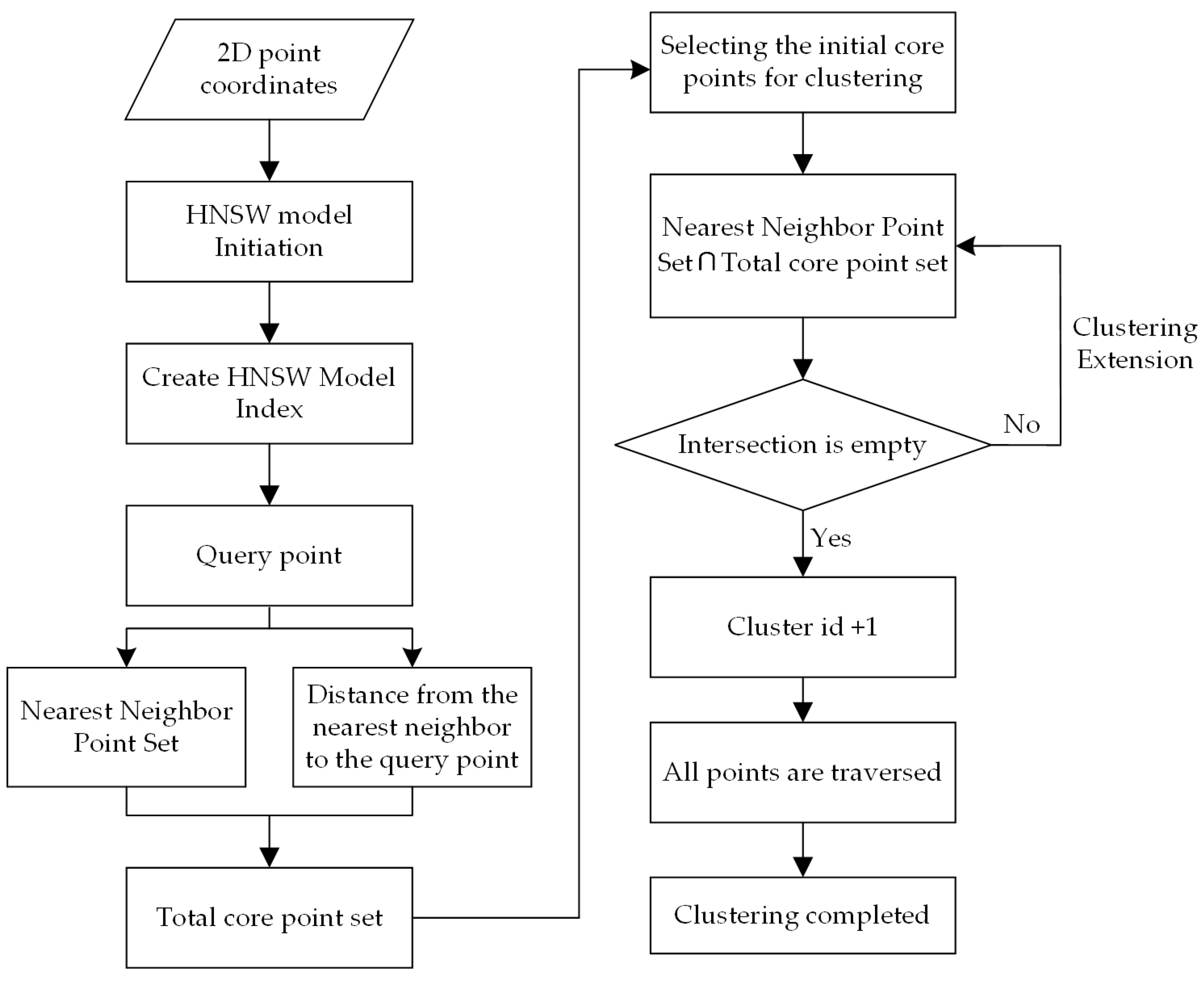
- (1)
- Select point A in dataset D, count all the points in the neighborhood eps of point A, and write the neighborhood as Numeps(A), if Numeps(A) ≥ MinPts, mark point as the core point and establish the cluster core point at the same time; if Numeps(A) < MinPts, the point is a noise point.
- (2)
- Select the next point within Numeps(A) in the neighborhood B(m, n), and add Numeps(B) to Numeps(A) in the same step as the previous one.
- (3)
- Repeat step 2 until all the points in the Numeps(A).
- (4)
- Repeat steps 1–3 until all points in dataset D are traversed and marked as core points or noise.
3.3. Hierarchical Navigable Small Worlds and DBSCAN
4. Results and Analysis
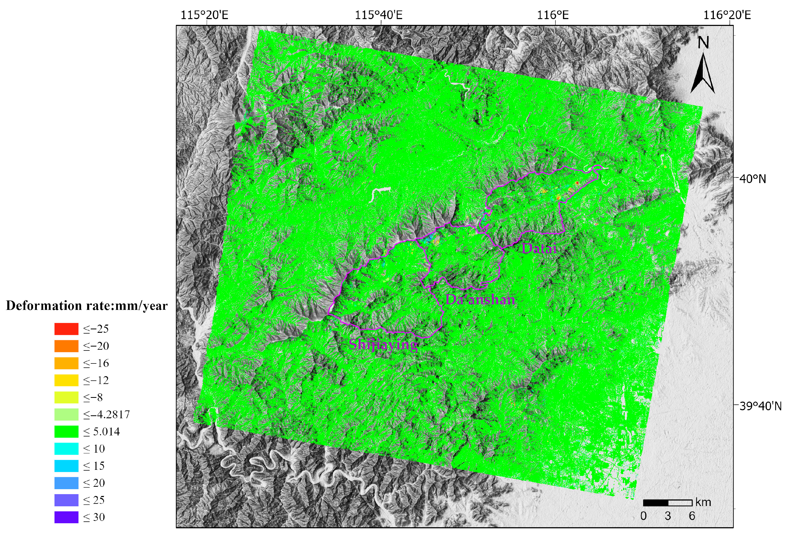
4.1. Result of IPTA Processing
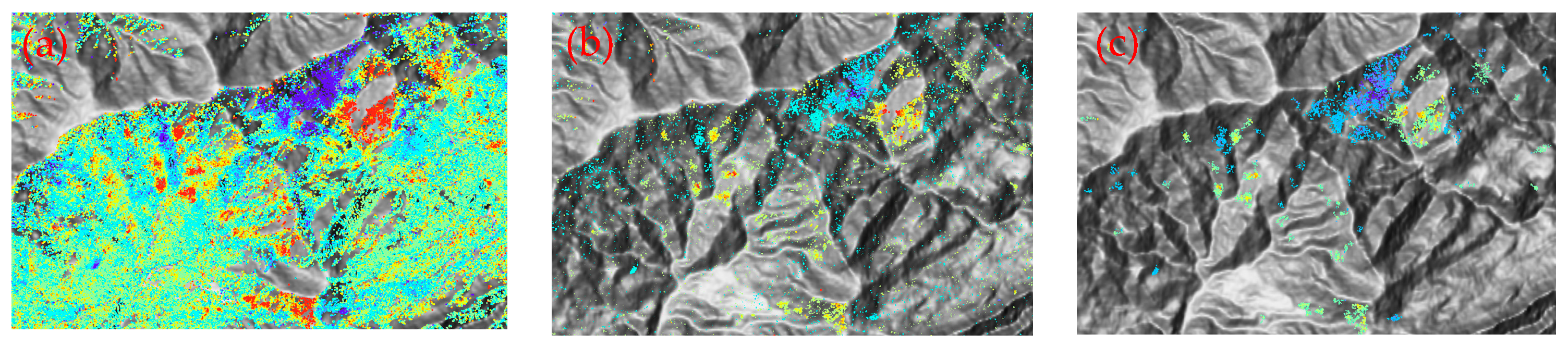
4.2. HNSW–DBSCAN
4.3. Comparison between Traditional DBSCAN and HNSW–DBSCAN
5. Discussion
6. Conclusions
- This paper proposes the HNSW–DBSCAN algorithm, which combines the HNSW and DBSCAN methods. The algorithm is tested using Beijing Xishan Mountain as the study area. The results show that the algorithm effectively removes spatial noise and greatly improves clustering efficiency while maintaining high accuracy compared with traditional methods.
- This paper introduces a method that combines slope units with clustering results to identify the slopes where deformation occurs efficiently. This approach aims to enhance InSAR decoding efficiency and enable the rapid targeting of deformation areas.
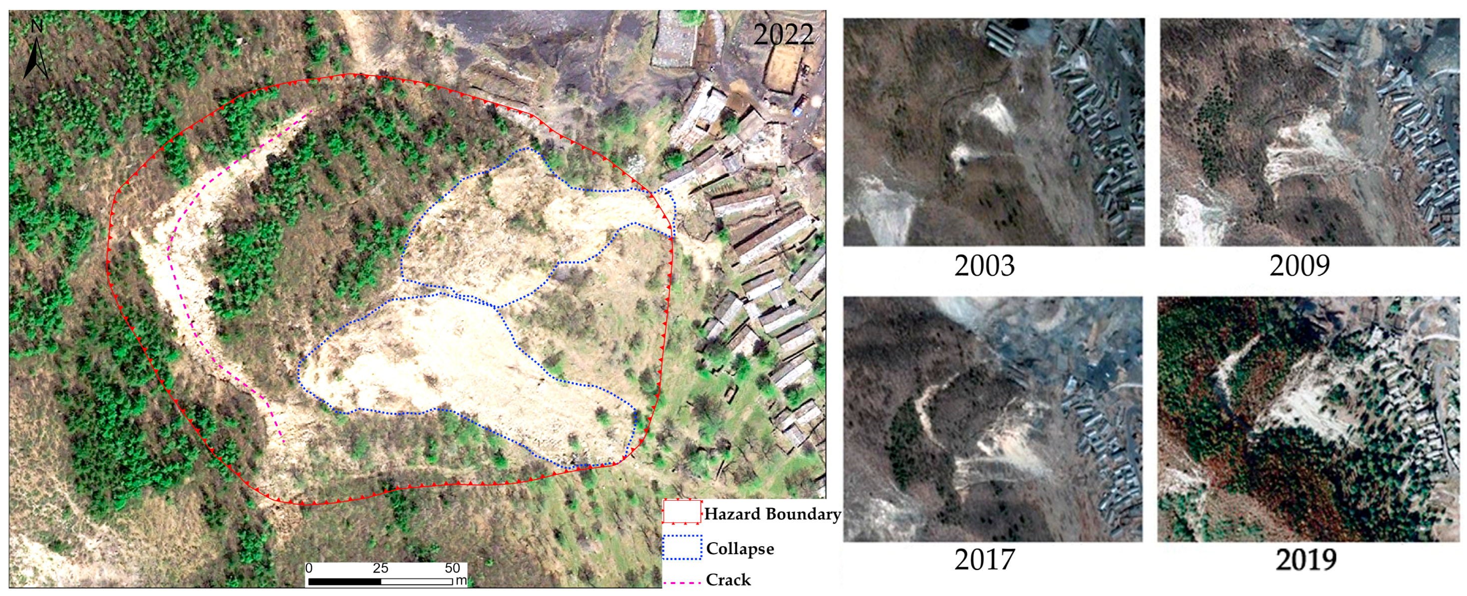
- IPTA technology was employed to monitor surface deformation in the Xishan area of Beijing. The accuracy of the results from IPTA technology in highly vegetation-covered mountainous areas was verified through in-conformity accuracy verification. Furthermore, field validation was conducted to confirm the decoded landslides, and the validation results were found to be consistent with the InSAR decoding results.
Author Contributions
Funding
Data Availability Statement
Acknowledgments
Conflicts of Interest
References
- Ministry of Natural Resources of the People’s Republic of China. Statistical Bulletin of China’s Natural Resources in 2022. Available online: https://www.mnr.gov.cn/sj/tjgb.html (accessed on 1 April 2023).
- Zhao, J.; Chen, Q.; Yang, Y.; Xu, Q. Coseismic Faulting Model and Post-Seismic Surface Motion of the 2023 Turkey–Syria Earthquake Doublet Revealed by InSAR and GPS Measurements. Remote Sens. 2023, 15, 3327. [Google Scholar] [CrossRef]
- Liu, Y.; Cao, W.; Shi, Z.; Yue, Q.; Chen, T.; Tian, L.; Zhong, R.; Liu, Y. Evaluation of Post-Tunneling Aging Buildings Using the InSAR Nonuniform Settlement Index. Remote Sens. 2023, 15, 3467. [Google Scholar] [CrossRef]
- Li, Z.; Dai, K.; Deng, J.; Liu, C.; Shi, X.; Tang, G.; Yin, T. Identifying Potential Landslides in Steep Mountainous Areas Based on Improved Seasonal Interferometry Stacking-InSAR. Remote Sens. 2023, 15, 3278. [Google Scholar] [CrossRef]
- Gao, H.; Xiong, L.; Chen, J.; Lin, H.; Feng, G. Surface Subsidence of Nanchang, China 2015–2021 Retrieved via Multi-Temporal InSAR Based on Long- and Short-Time Baseline Net. Remote Sens. 2023, 15, 3253. [Google Scholar] [CrossRef]
- Kumar Maurya, V.; Dwivedi, R.; Ranjan Martha, T. Site scale landslide deformation and strain analysis using MT-InSAR and GNSS approach—A case study. Adv. Space Res. 2022, 70, 3932–3947. [Google Scholar] [CrossRef]
- Liu, X.; Zhao, C.; Zhang, Q.; Lu, Z.; Li, Z.; Yang, C.; Zhu, W.; Liu-Zeng, J.; Chen, L.; Liu, C. Integration of Sentinel-1 and ALOS/PALSAR-2 SAR datasets for mapping active landslides along the Jinsha River corridor, China. Eng. Geol. 2021, 284, 106033. [Google Scholar] [CrossRef]
- Dong, J.; Liao, M.; Xu, Q.; Zhang, L.; Tang, M.; Gong, J. Detection and displacement characterization of landslides using multi-temporal satellite SAR interferometry: A case study of Danba County in the Dadu River Basin. Eng. Geol. 2018, 240, 95–109. [Google Scholar] [CrossRef]
- Kiseleva, E.; Mikhailov, V.; Smolyaninova, E.; Dmitriev, P.; Golubev, V.; Timoshkina, E.; Hooper, A.; Samiei-Esfahany, S.; Hanssen, R. PS-InSAR Monitoring of Landslide Activity in the Black Sea Coast of the Caucasus. Procedia Technol. 2014, 16, 404–413. [Google Scholar] [CrossRef]
- Dong, J.; Zhang, L.; Liao, M.; Gong, J. Improved correction of seasonal tropospheric delay in InSAR observations for landslide deformation monitoring. Remote Sens. Environ. 2019, 233, 111370. [Google Scholar] [CrossRef]
- Novellino, A.; Cesarano, M.; Cappelletti, P.; Di Martire, D.; Di Napoli, M.; Ramondini, M.; Sowter, A.; Calcaterra, D. Slow-moving landslide risk assessment combining Machine Learning and InSAR techniques. Catena 2021, 203, 105317. [Google Scholar] [CrossRef]
- Zhou, Z.; Yao, X.; Ren, K.; Liu, H. Formation mechanism of ground fissure at Beijing Capital International Airport revealed by high-resolution InSAR and numerical modelling. Eng. Geol. 2022, 306, 106775. [Google Scholar] [CrossRef]
- Cai, J.; Liu, G.; Jia, H.; Zhang, B.; Wu, R.; Fu, Y.; Xiang, W.; Mao, W.; Wang, X.; Zhang, R. A new algorithm for landslide dynamic monitoring with high temporal resolution by Kalman filter integration of multiplatform time-series InSAR processing. Int. J. Appl. Earth Obs. 2022, 110, 102812. [Google Scholar] [CrossRef]
- Lu, P.; Bai, S.; Tofani, V.; Casagli, N. Landslides detection through optimized hot spot analysis on persistent scatterers and distributed scatterers. Isprs J. Photogramm. 2019, 156, 147–159. [Google Scholar]
- Ma, P.; Li, T.; Fang, C.; Lin, H. A tentative test for measuring the sub-millimeter settlement and uplift of a high-speed railway bridge using COSMO-SkyMed images. Isprs J. Photogramm. 2019, 155, 1–12. [Google Scholar] [CrossRef]
- Chen, F.; Lin, H.; Zhou, W.; Hong, T.; Wang, G. Surface deformation detected by ALOS PALSAR small baseline SAR interferometry over permafrost environment of Beiluhe section, Tibet Plateau, China. Remote Sens. Environ. 2013, 138, 10–18. [Google Scholar] [CrossRef]
- Wang, Y.; Feng, G.; Li, Z.; Xu, W.; Wang, H.; Hu, J.; Liu, S.; He, L. Estimating the long-term deformation and permanent loss of aquifer in the southern Junggar Basin, China, using InSAR. J. Hydrol. 2022, 614, 128604. [Google Scholar] [CrossRef]
- Haibo, Z.; Zongchun, L.; Bing, X. Ground Subsidence Monitoring Using Interferometric Point Target Analysis. J. Geomat. Sci. Technol. 2016, 33, 145–149. [Google Scholar]
- Rongrong, D.; Jia, X.U.; Xiaobin, L.; Kang, X.U. Monitoring of surface subsidence using PSInSAR with TerraSAR-X high-resolution data. Remote Sens. Land Resour. 2015, 27, 158–164. [Google Scholar]
- Gatsios, T.; Cigna, F.; Tapete, D.; Sakkas, V.; Pavlou, K.; Parcharidis, I. Copernicus Sentinel-1 MT-InSAR, GNSS and Seismic Monitoring of Deformation Patterns and Trends at the Methana Volcano, Greece. Appl. Sci. 2020, 10, 6445. [Google Scholar] [CrossRef]
- Chen, Z.; Zhang, L.; Zhang, G. An improved InSAR image co-registration method for pairs with relatively big distortions or large incoherent areas. Sensors 2016, 16, 1519. [Google Scholar] [CrossRef]
- Wang, S.; Zhang, G.; Chen, Z.; Xu, Z.; Liu, Y. A refined parallel stacking InSAR workflow for large-scale deformation fast extraction—A case study of Tibet. Geocarto Int. 2022, 37, 16074–16085. [Google Scholar] [CrossRef]
- Bakon, M.; Oliveira, I.; Perissin, D.; Sousa, J.; Papco, J. A data mining approach for multivariate outlier detection in heterogeneous 2D point clouds: An application to post-processing of multi-temporal InSAR results. In Proceedings of the 2016 IEEE International Geoscience and Remote Sensing Symposium (IGARSS), Beijing, China, 10–15 July 2016; pp. 56–59. [Google Scholar]
- Zhang, P.; Guo, Z.; Guo, S.; Xia, J. Land Subsidence Monitoring Method in Regions of Variable Radar Reflection Characteristics by Integrating PS-InSAR and SBAS-InSAR Techniques. Remote Sens. 2022, 14, 3265. [Google Scholar] [CrossRef]
- Talib, O.; Shimon, W.; Sarah, K.; Tonian, R. Detection of sinkhole activity in West-Central Florida using InSAR time series observations. Remote Sens. Environ. 2022, 269, 112793. [Google Scholar] [CrossRef]
- Han, J.; Yang, H.; Liu, Y.; Lu, Z.; Zeng, K.; Jiao, R. A Deep Learning Application for Deformation Prediction from Ground-Based InSAR. Remote Sens. 2022, 14, 5067. [Google Scholar] [CrossRef]
- Liu, Y.; Yang, H.; Fan, J.; Han, J.; Lu, Z. NL-MMSE: A Hybrid Phase Optimization Method in Multimaster Interferogram Stack for DS-InSAR Applications. IEEE J.-Stars. 2022, 15, 8332–8345. [Google Scholar] [CrossRef]
- Malkov, Y.A.; Yashunin, D.A. Efficient and Robust Approximate Nearest Neighbor Search Using Hierarchical Navigable Small World Graphs. IEEE Trans. Pattern Anal. Mach. Intell. 2020, 42, 824–836. [Google Scholar] [CrossRef]
- Alvioli, M.; Marchesini, I.; Reichenbach, P.; Rossi, M.; Ardizzone, F.; Fiorucci, F.; Guzzetti, F. Automatic delineation of geomorphological slope units with r.slopeunits v1.0 and their optimization for landslide susceptibility modeling. Geosci. Model Dev. 2017, 9, 3975–3991. [Google Scholar] [CrossRef]
- Jiao, R.; Wang, S.; Yang, H.; Guo, X.; Han, J.; Pei, X.; Yan, C. Comprehensive Remote Sensing Technology for Monitoring Landslide Hazards and Disaster Chain in the Xishan Mining Area of Beijing. Remote Sens. 2022, 14, 4695. [Google Scholar] [CrossRef]


| Month | 1 | 2 | 3 | 4 | 5 | 6 | 7 | 8 | 9 | 10 | 11 | 12 | |
|---|---|---|---|---|---|---|---|---|---|---|---|---|---|
| Year | |||||||||||||
| 2016 | / | / | / | / | / | / | / | / | 24 | 18 | 11 | 29 | |
| 2017 | 22 | 15 | 11 | 4/28 | 22 | 15 | / | / | 19 | 13 | 6/30 | 24 | |
| 2018 | 17 | 10 | 6/30 | 23 | 17 | 10 | 28 | 21 | 14 | 8 | 1/25 | / | |
| 2019 | 12 | 5 | 1 | 18 | 12 | 5 | 23 | 16 | 9 | 3/27 | 20 | 14 | |
| 2020 | 7 | 24 | 19 | 12 | 6/30 | 23 | 17 | 10 | 3/27 | 21 | / | 8 | |
| 2021 | 1/25 | 18 | 14 | 7 | 25 | 18 | 12 | 5 | 22 | 16 | 9 | 3 | |
| 2022 | / | 13 | / | 2/26 | 20 | 13 | 7/31 | 24 | 17 | ||||
| CPU | RAM | GPU | Solid State Drives |
|---|---|---|---|
| I9-12900KS | 128 G | GTX 1660 | 2 T |
| Total Pixels | <100 | <400 | <1000 | <2000 | ≥2000 | Total |
|---|---|---|---|---|---|---|
| Number | 10 | 14 | 12 | 9 | 8 | 53 |
| Data | Adjust Rand Index | Homogeneity | Completeness | V-Measure |
|---|---|---|---|---|
| d6 | 98.7% | 96.3% | 96.4% | 96.4% |
| l3 | 98.7% | 97.7% | 97.5% | 97.6% |
| t4 | 98.6% | 97.3% | 97.4% | 97.4% |
| t7 | 96.4% | 94.7% | 92.1% | 93.4% |
Disclaimer/Publisher’s Note: The statements, opinions and data contained in all publications are solely those of the individual author(s) and contributor(s) and not of MDPI and/or the editor(s). MDPI and/or the editor(s) disclaim responsibility for any injury to people or property resulting from any ideas, methods, instructions or products referred to in the content. |
© 2023 by the authors. Licensee MDPI, Basel, Switzerland. This article is an open access article distributed under the terms and conditions of the Creative Commons Attribution (CC BY) license (https://creativecommons.org/licenses/by/4.0/).
Share and Cite
Han, J.; Guo, X.; Jiao, R.; Nan, Y.; Yang, H.; Ni, X.; Zhao, D.; Wang, S.; Ma, X.; Yan, C.; et al. An Automatic Method for Delimiting Deformation Area in InSAR Based on HNSW-DBSCAN Clustering Algorithm. Remote Sens. 2023, 15, 4287. https://doi.org/10.3390/rs15174287
Han J, Guo X, Jiao R, Nan Y, Yang H, Ni X, Zhao D, Wang S, Ma X, Yan C, et al. An Automatic Method for Delimiting Deformation Area in InSAR Based on HNSW-DBSCAN Clustering Algorithm. Remote Sensing. 2023; 15(17):4287. https://doi.org/10.3390/rs15174287
Chicago/Turabian StyleHan, Jianfeng, Xuefei Guo, Runcheng Jiao, Yun Nan, Honglei Yang, Xuan Ni, Danning Zhao, Shengyu Wang, Xiaoxue Ma, Chi Yan, and et al. 2023. "An Automatic Method for Delimiting Deformation Area in InSAR Based on HNSW-DBSCAN Clustering Algorithm" Remote Sensing 15, no. 17: 4287. https://doi.org/10.3390/rs15174287