Article

Quantifying Water Impoundment-Driven Air Temperature Changes in the Dammed Jinsha River, Southwest China

1
Chengdu Institute of Biology, Chinese Academy of Sciences, Chengdu 610041, China
2
University of Chinese Academy of Sciences, Beijing 100049, China
3
State Key Laboratory of Hydro-Science and Engineering, Department of Hydraulic Engineering, Tsinghua University, Beijing 100084, China
4
Institute of Information Engineering, Chinese Academy of Sciences, Beijing 100195, China
*
Author to whom correspondence should be addressed.
Remote Sens. 2023, 15(17), 4280; https://doi.org/10.3390/rs15174280
Submission received: 16 July 2023 / Revised: 23 August 2023 / Accepted: 29 August 2023 / Published: 31 August 2023

Abstract

:
A number of previous studies have contributed to a better understanding of the thermal impacts of dam-related reservoirs on stream temperature, but very few studies have focused on air temperature, especially at the catchment scale. In addition, due to the lack of quantitative analysis, the identification of the effects of water impoundment on regional air temperature is still lacking. We investigated the impacts of reservoirs on the regional air temperature changes before and after two large dam constructions in the lower Jinsha River located in southwest China, by using a 40 year record of reanalysis data at 90 m resolutions. Furthermore, the long short-term memory (LSTM) model was also employed to construct an impoundment effect on the temperature (IET) index. Research results indicate that compared to the pre-impoundment period (1980–2012), the variations in the air temperature at the catchment scale were reduced during the post-impoundment period (2013–2019). The annual maximum air temperature decreased by 0.4 °C relative to the natural regimes. In contrast, the cumulative effects of dam-related reservoirs increased the annual mean and minimum air temperature by 0.1 °C and 1.0 °C, respectively. Warming effects prevailed during the dry season and in the regions with high elevations, while cooling effects dominated within a 4 km buffer of the reservoirs. Therefore, this study offers important insights about the impacts of anthropogenic impoundments on air temperature changes, which could be useful for policymakers to have a more informed and profound understanding of local climate changes in dammed areas.

1. Introduction

Anthropogenic impoundments (e.g., dams, reservoirs, and ponds) are often considered important contributors to the development of human societies by providing multiple services including hydropower generation, flood control, and water supply [1]. Since the 1950s, anthropogenic impoundments have been flourishing as a response to the ever-growing requirements for water and energy [2]. However, despite their societal significance, anthropogenic impoundments are also associated with several serious environmental problems, including river system fragmentation [3], water diversion [4], changes in flow conditions [5], decreased nutrient deliveries [6], interruptions of fish migrations [7], reservoir flushing [8], alterations in bio-geochemical cycling [9], and disturbing climate regimes [10]. Among them, the thermal variations associated with the dammed reservoirs are of considerable interest. This is because the dams and reservoirs substantially alter the hydrological and thermal regimes of the river, as well as the surface energy balance of the region [11].
The dammed hydropower, as one of the typical anthropogenic impoundments, generates power by using a dam that changes the natural flow of a river. It provides multiple benefits and values to economic prosperity and social well-being by acting as a primary and low-cost renewable source of energy worldwide [12]. Approximately two-thirds of the rivers in the world have dammed reservoirs [13]. It is physically reasonable to expect a gradual air and water temperature variation in the impounded river basin. This is directly attributed to the changing atmospheric conditions due to heat transfers, which, in turn, occur because of the surface and internal thermodynamic phenomena of reservoirs [10]. As a result, numerous studies have been carried out to analyze the thermal responses caused by the generation of dammed hydropower. Nevertheless, these previous studies usually focused on water temperature variations associated with dams and reservoirs, including the reduction in magnitude, frequency, duration, and variability of water temperature, and weakening interactions at the air/water interface due to the altered heat exchange rate [14,15]. Although reservoirs exhibit an enormous capacity to regulate air temperature regimes, the relationship between water impoundment and air temperature remains poorly understood [10,16,17].
Air temperature is a sensitive indicator of the surface energy balance, as well as a crucial parameter in biogeochemical and biophysical feedbacks to the climate system [18]. Several investigations have been carried out to realize the impact of dams and associated reservoirs on air temperature. For instance, Zeng et al. [19] found that the annual average air temperature increased in the Three Gorges Dam reservoir area. Another study performed by Fonseca and Santos [20] on the Sabor River demonstrated that the daily and seasonal temperature decreased in the post-impoundment period. Miller et al. [21] modeled the climate changes for eight weeks in the Three Gorges Dam area and suggested that the decreased local surface and air temperature likely occurred because the reservoir acted as a potential evaporating surface. Irambona et al. [22] found that reservoirs induced localized 2 m temperature warming in winter and cooling in the summer in the La Grande River watershed. Wang et al. [18] revealed that the reservoir had both warming and cooling effects on the surface temperature in different parts of the dry–hot valley. Zhao et al. [23] explored the potential connection between reservoir characteristic factors and meteorological variables at the global scale, and suggested that they possibly have contrasting effects on the air temperature. However, compared to the well-informed water temperature variations, a significant delay in the knowledge of air temperature changes is noticeable. Hence, there is still a major research gap in the regional-scale understanding of dam-induced air temperature alterations, and it is critically required to determine how artificial reservoirs influence the air temperature at the catchment scale [17].
The lower Jinsha River, as the upper reaches of the Yangtze River, is one of the largest hydropower production regions in China [24]. It has a hydropower generation capacity of 40 million kW, which is twice that of the Three Gorges Reservoir [25]. As a consequence, the lower Jinsha River has become one of the most highly modified rivers in the world [18]. The dams and related reservoirs in the lower Jinsha River may change the local air temperature patterns and further affect the thermal regime of the middle and lower Yangtze River. Moreover, these cascade reservoirs in the lower Jinsha River are more pronounced than those of an individual dam [26], and, thus, they will further change the annual or seasonal thermal regimes of the river basin. By mostly considering the Gezhouba Dam and the Three Gorges Dam in the middle river, previous investigations have examined the effects of dam-related reservoirs on the thermal regime in the Yangtze River, however, the effects of water impoundment on the local air temperature in the lower Jinsha River remain largely unclear [18]. Therefore, if water impoundments inadvertently modify climate patterns in impounded river basins, understanding the influence exerted by reservoirs in the lower Jinsha River will be key.
Over the past two decades, a long short-term memory (LSTM) model has been successfully developed and extensively employed for temperature forecasting [27]. As a deep learning model, LSTM is composed of multiple simple nonlinear models, and the original input data are learned layer-by-layer to establish complex equations between variables [28,29]. Thus, to quantify the impact of water impoundment on air temperature, LSTM can be utilized to predict future temperature under the no impoundment scenario through historical data, and the difference between actual and predicted data can be used to define the impacts.
Hence, in this study, we tried to find an answer to the following open question: What is the probable influence of large dams and related reservoirs on local air temperature changes? The novelty and primary contribution of this study were to highlight complexities in the response of the local air temperature to water impoundments. This has not been previously fully investigated in the literature, and only site-specific analyses have already paid attention to it. Specifically, the objectives of this study were as follows: (a) explaining spatiotemporal patterns of local air temperature in pre- and post-impoundment periods; (b) developing a predictive model based on the LSTM method and reconstructing air temperatures in the absence of impoundments; (c) assessing the influence of dams and related reservoirs on local air temperatures by comparing observed and predicted values in the post-impoundment period. The findings of this study can be beneficial to develop a more general understanding of the impacts of anthropogenic impoundments on air temperature variations, because global change changes will likely exacerbate them.

2. Materials and Methods
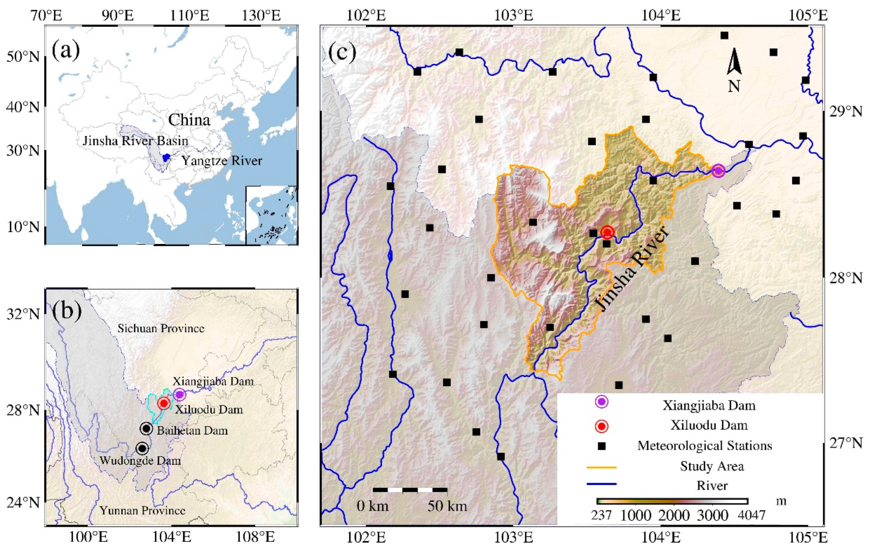
2.1. Study Area

Four large hydropower stations including Xiangjiaba, Xiluodu, Baihetan, and Wudongde have been built in the lower Jinsha River. They are all ranked among the top five largest hydropower stations in China, with a total installed capacity of 42.96 gigawatt [30]. Specifically, the Xiangjiaba, Xiluodu, Baihetan, and Wudongde reservoirs started the impoundment in December 2012, May 2013, April 2021, and January 2020, respectively [31]. Consequently, by considering the late impoundment time of the Baihetan and Wudongde hydropower stations, we only focused on the thermal disturbance of the Xiangjiaba and Xiluodu reservoirs. The water storage capacity is 5.16 billion m3 for Xiangjiaba Reservoir and 12.67 billion m3 for Xiluodu Reservoir.
The river basin (27.37°N–28.90°N, 102.83°E–104.42°E) where Xiangjiaba and Xiluodu hydropower stations are located was selected as a case study area, spanning two administrative provinces of Sichuan and Yunnan, and is approximately 11,167.70 km2 in size (Figure 1). Elevations vary greatly ranging from around 240 m in the northeastern region to more than 4000 m in the southwestern region, showing complicated topographic structures. The study area has a subtropical climate with the dry season and the wet season [32]. The dry season runs from November to April, and the wet season stretches from May to October. Due to the great changes in terrain, elevations, and latitudes, the climatic conditions in the catchment are complex. Its mean annual precipitation is 732–1028 mm and its mean temperature is 13–18 °C, presenting a decreasing and increasing trend from northeast to southwest of the basin, respectively [33]. The study area is characterized by two distinct climate areas and vegetation, ranging from the monsoon region with subtropical evergreen broad-leaved vegetation in the northeastern zone, to the dry–hot valley with Savanna-like vegetation in the southwestern zone [34].

2.2. Data Sources

2.2.1. Meteorological Data

In our study region within the 100 km buffer zone [35], daily mean (Tmean), maximum (Tmax), and minimum (Tmin) air temperatures of 47 meteorological stations from January 1980 to December 2019 were collected from the China Meteorological Data Service Centre (http://data.cma.cn, accessed on 8 June 2022). After excluding four stations with discontinuous time series for one or more calendar months, we reserved 43 meteorological stations for analysis as indicated by the black rectangles in Figure 1.
To ensure the reliability and continuity of the air temperature data, the Pauta criterion method was employed to detect outliers, with 37 (0.24%), 335 (2.18%), and 10 (0.07%) outliers detected for Tmean, Tmax, and Tmin, respectively. The linear interpolation method was further utilized to replace them and the original missing values [36], and the results can be seen in Figure 2. The annual and seasonal air temperatures were acquired by averaging the corresponding month’s temperatures. Hence, four air temperature datasets at monthly, annual, dry season, and wet season scales were generated. It is pertinent to note that the statistical analysis or mapping in this study was all implemented using Python 3.9 software.

2.2.2. Terrain Morphology Data

The digital elevation model (DEM) at the spatial resolution of 90 m was used to represent the terrain of the study area, which was obtained from the NASADEM digital elevation dataset via the Google Earth Engine (GEE) platform [37].

2.3. Methods

The methodological framework of the whole research is depicted in Figure 3a. The specific methods employed are described as follows.

2.3.1. Interpolation Methods

To generate the air temperature grid surface datasets at annual, dry season, and wet season scales based on the meteorological data, the Australian National University Spline (ANUSPLIN) model was adopted. The ANUSPLIN model provides a means for the interpolation of noisy multi-variate data using thin-plate smoothing splines. It has been widely employed to develop geographically continuous climate grid surface data from weather station data and topographic variables that primarily include longitude, latitude, and elevation. The ANUSPLIN calculation formula was described by Hutchinson [38] as follows:
Z i = f x i + b T y i + ε i ( i = 1 , , n )
where x i represents a p-dimensional vector of spline independent variables, f denotes a smoothing function of the x i , each y i represents a p-dimensional vector of independent covariates, b stands for an unknown p-dimensional vector of coefficients of the y i , and each ε i represents an independent, zero mean error term.

2.3.2. Trends Analysis

The Theil–Sen estimator and Mann–Kendall (MK) trend test were integrated to identify the air temperature trend variations on the pixel scale during both the pre-impoundment period (1980–2012) and the post-impoundment period (2013–2019). The combined results were classified into the following four distinct categories: non-significant increase (Ni), significant increase (Si), non-significant decrease (Nd), and significant decrease (Sd). The Theil–Sen estimator is a robust nonparametric statistics method for estimating the slope of a trend [39]. Its calculation formula is as follows:
S = M e d i a n T j T i j i , i < j
where S signifies the Theil–Sen median slope, and T i and T j symbolize the air temperature at time i and j of each pixel, respectively. When S > 0 , it indicates an increasing trend, and when S < 0 , it indicates a decreasing trend.
The MK trend test is a nonparametric test method for quantifying the significance of a trend. The Z statistic is usually calculated initially. By checking within the standard normal distribution table, the p-value can be obtained according to the Z statistic. The p-value is utilized as a likelihood indicator to measure the significance of a trend. The smaller the p-value, the greater the likelihood for the temperature series to have a significant trend. We set the significance level α to 5%, and when p < 0.05 , the trend was considered significant; otherwise, it was considered not significant. Specific details on the calculation procedure can be found in Liu and Menzel [40].
Additionally, to detect and identify the time when significant changes in air temperature occurred in the time series of 1980–2019, the MK mutation test was also adopted. U F K was used to test the mutation of trends in the air temperature series, while U B K was calculated with the reverse series of U F K . The U F K and U B K curves were plotted under annual, dry season, and wet season scales. The mutation point of the temperature series can be identified as the point where the curves of U F K and U B K intersect within the confidence interval ( U F = 0.05 / 2 = 1.96 ). Further detailed information regarding the MK mutation test can be found in Hong and Zhang [41].

2.3.3. Quantitative Analysis of Impoundment Effects

We developed an impoundment effect on the temperature (IET) index to further quantify the impact of water impoundments on regional air temperature. We defined the IET index as the difference value between actual air temperature and predicted air temperature. The actual air temperature was simulated using the ANUSPLIN model in the post-impoundment period (2013–2019). Predicted air temperature in the post-impact period was simulated by the LSTM model, by using the actual air temperature data during the pre-impoundment period (1980–2012). Thus, the effects of water impoundment on air temperature were simulated as follows:
I E T = A T V P T V
where A T V stands for the actual temperature value (°C), and P T V represents the predicted temperature value (°C). When I E T > 0 , the water impoundment has a warming effect on air temperatures, whereas when I E T < 0 , the impoundment has a cooling effect.
LSTM model can capture the nonlinear features of long time-series data and can avoid the gradient vanishing and exploding issues encountered in the conventional recurrent neural network (RNN) [42]. It consists of an input layer, an output layer, and a hidden layer. The input data are sequentially processed through these three layers to acquire pertinent information and eliminate extraneous information, thereby achieving an accurate prediction. The hidden layer is composed of four units: the forget gate, the input gate, and the output gate, as well as the memory state unit. The structure of the hidden layer is critical for filtering the data and can be composed of multiple layers (Figure 3b). For more detailed information regarding the LSTM model, please refer to Hochreiter and Schmidhuber [43].
To enhance the accuracy of our prediction, the LSTM model was designed with two layers, in which the output of the first LSTM layer acted as the input for the second LSTM layer [44]. The input dataset of the LSTM model aggregated 10,000 temperature series samples, which were randomly extracted from all pixels of the historical actual grid surface dataset (384 months, from 1980 to 2012). It was then partitioned into a training set (90%) and a testing set (10%) based on the sample locations, which were employed to train the model and assess the model performance, respectively. After training and testing, the predicted air temperature dataset (2013–2019) was generated via the constructed LSTM model by inputting the historical dataset (1980–2012). It should be noted that the predicted grid surface datasets of Tmean, Tmax, and Tmin were generated by the three LSTM models.

2.3.4. Model Assessment

We employed the 10-fold cross-validation method to evaluate the effectiveness of the ANUSPLIN model, which has been broadly employed to evaluate the model performance [45]. The original observation data at 43 meteorological stations were randomly divided into ten subsets. We further used nine of those ten subsets as the training datasets, which were inputted into ANUSPLIN models, and reserved one-tenth as the observed datasets to test the models. The simulated datasets were extracted through the training outputs at the corresponding locations of the observed datasets. These processes were iterated ten times. Hence, ten different combinations of stimulated and observed datasets were generated, and the final performance of the ANUSPLIN model was determined by the average discrepancy between each pair.
Furthermore, we calculated the mean absolute error ( M A E ), root mean square error ( R M S E ), and coefficient of determination ( R 2 ) to evaluate the performance of the ANUSPLIN model and LSTM model [46]. The calculation formulas were as follows:
R M S E = 1 n i = 1 n ( T s T o )
M A E = 1 n i = 1 n | T s T o |
R 2 = i = 1 n ( T s T o ¯ ) 2 i = 1 n ( T o T o ¯ ) 2
where n represents the number of samples, T s denotes the simulated data obtained from the model, and T o stands for the observed data from the testing sets. The distribution range of R M S E and M A E values is [0, +∞), while the range of R 2 values is [0, 1]. A higher level of precision is deduced in the evaluated model when the R M S E and M A E values approach 0 and the R 2 value approaches 1.

3. Results

3.1. Evaluation of the ANUSPLIN Model Performance

Figure 4 shows the M A E , R M S E , and R 2 values of each air temperature indicator at annual and seasonal scales. For the interpolated air temperature grid datasets at the annual scale, the mean R M S E was 0.45 °C (the values ranged from 0.31 °C to 0.60 °C), the mean M A E was 0.07 °C (the values were about 0.1 °C), and the R 2 was 0.94 (the values were within the range of 0.93–0.96). The mean RMSE for the interpolated air temperature grid datasets for the dry season was 0.40 °C (the values were within the range of 0.31–0.50 °C), and for the wet season was 0.45 °C (the values ranged from 0.37 °C to 0.52 °C). Compared to Tmean and Tmin, Tmax had a higher interpolation accuracy, with smaller R M S E and M A E values. In addition, as the magnitude of air temperature varied for different seasons, the R M S E s (or M A E s ) of the interpolated grid datasets were smaller in the dry season than in the wet season, and the R 2 remained reasonably constant with all values greater than 0.93 and close to 1 across the study period. The results prove that the ANUSPLIN method is reliable for the air temperature estimation in the lower Jinsha River Basin.

3.2. Air Temperature Changes before and after Impoundments

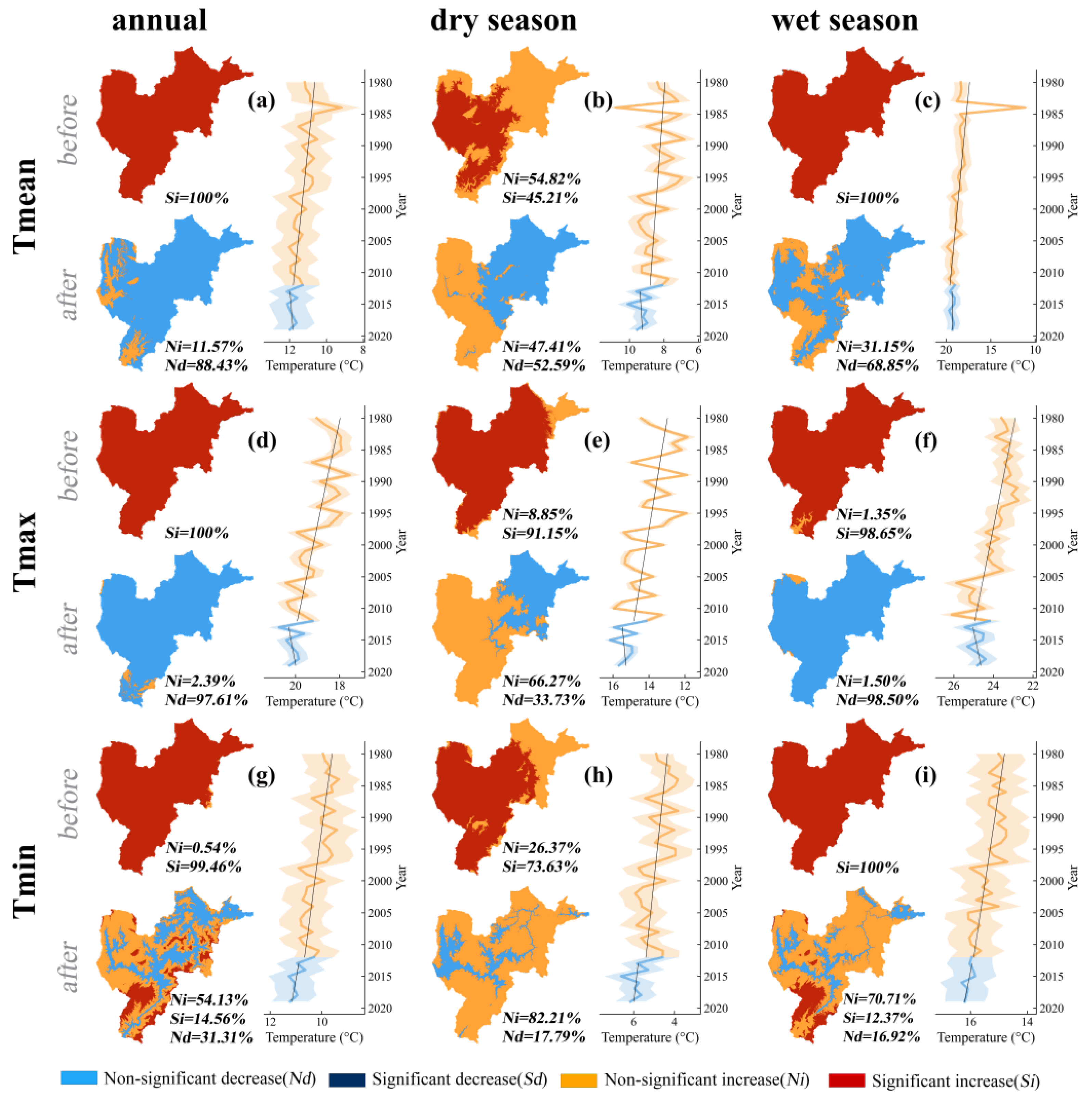
3.2.1. Spatiotemporal Patterns

Figure 5 exhibits the comparison of air temperature change trends for the pre-impoundment period (1980–2012) and the post-impoundment period (2013–2019). It can be observed that the air temperature shows an overall significant increase before the water impoundment, while after the impoundments, the Tmean and Tmax experience an average decrease, and the Tmin displays an average increase. All air temperature indicators generally transform from a significant trend to a non-significant trend in most areas of the catchment. Note that some regions still show a significant increase for Tmin after the impoundment.
As for annual Tmean, 88.43% of the study area experience a non-significant decrease, particularly in the central and eastern regions (Figure 5a). A similar spatial pattern also occurs in the dry season (52.59%, Figure 5b) and wet season (68.85%, Figure 5c). However, it is worth noting that some western regions exhibit a non-significant increase in the dry season (0.47 °C year−1), and a non-significant decrease in the wet season (0.69 °C year−1), which results in a non-significant decrease for annual scale. In addition, 97.61% of the catchment’s Tmax shows a non-significant decrease after water impoundments (Figure 5d). This phenomenon is attributed to the presence of a non-significant decrease in both dry and wet seasons (Figure 5e,f). Finally, Tmin exhibits a more conspicuous spatial heterogeneity than Tmean and Tmax after water impoundments. The regions with a Tmin decrease (i.e., a non-significant decrease of 54.13%, Figure 5g) predominantly appear around reservoirs in both dry and wet seasons (17.79% and 16.92%, respectively, Figure 5h,i). However, the annual and wet seasonal Tmin maintains a significant increase similar to the trend before impoundments (14.56% and 12.37%, respectively, Figure 5g), which indicates small variations in Tmin in comparison to Tmean and Tmax.

3.2.2. Change-Points Detection

To detect and identify the time in which significant changes in air temperatures occurred, the temperature indicators were identified by using the MK mutation test at both annual and seasonal scales. It can be observed that the annual changes for Tmean, Tmax, and Tmin are quite similar to the seasonal changes (Figure 6). There is no significant change point for each indicator at the annual scale, while mutations occur at both the dry and wet season scales. In particular, the significant changes occurred in 2013 for Tmean, and in 2006 and 2008 for Tmax. Even though U F K and U B K curves of Tmin intersect, the U F K statistics do not exceed the critical line (Figure 6g–i), thus, no mutations could be confirmed for the Tmin. Notably, the mutation time for the Tmean during the dry season in 2012 coincided with the impounding time of the Xiluodu Reservoir (Figure 6b).
Overall, only one significant change point was observed at the dry season scale after the water impoundments. This phenomenon implied that after the water impoundment in the lower Jinsha River Basin, the air temperature variations were alleviated.

3.3. Effects of Water Impoundments on Air Temperature

3.3.1. Evaluation of the LSTM Model Performance

To evaluate the performance of LSTM models in predicting each air temperature grid surface dataset (Figure 7), we used the testing sets from monthly temperature grid surface datasets of the 1980–2012 period. The monthly LSTM forecast was well supported by actual data. It can be seen that both the M A E and R M S E values of the three models hover around 0.1 °C and the R 2 values are close to 1, reflecting the robustness of LSTM models. We further utilized the least squares method to determine the best linear fit in each scatterplot. The LSTM models tend to slightly underestimate the air temperature (the fitting slope for the Tmean is 1.00062, for the Tmax is 1.00058, and for the Tmin is 1.00091). However, they are all close to 1, reflecting the remarkable similarities between actual data and LSTM forecast, which further confirms the high reliability and accuracy of the LSTM models in predicting Tmean, Tmax, and Tmin datasets.

3.3.2. Patterns of the IET Index

Figure 8 displays the spatial distribution of the IET index at annual and seasonal scales. According to Figure 8, the IET index had both positive and negative values across the catchment and at different scales, suggesting that both warming and cooling effects existed. Generally, there was a similar pattern for Tmean and Tmax, while there was a different pattern for Tmean. In particular, for the annual Tmean, the average IET was 0.1 °C, with 51% of the catchment showing a warming effect (IET > 0) after water impoundment (chiefly in the western region), while the remaining 49% (principally in the eastern region) exhibited a cooling effect with IET < 0 (Figure 8a). The cooling effect in the eastern region was mainly attributed to the negative IET index in both the dry and wet seasons. Specifically, 44% (out of 80%) of the regions show a substantially positive reduction during the wet season, while 41% (out of 74%) of the regions exhibit a substantially positive increase in the western region during the dry season (Figure 8b,c).
The average IET value for the annual Tmax was −0.4 °C, indicating that water impoundment gave rise to an overall 0.4 °C reduction. This was mostly caused by significant temperature decreases in 81% of the basin, especially during the wet season with a magnitude of around 2 °C reduction primarily distributed in surrounding areas of the reservoirs (Figure 8d–f). It is worth mentioning that the annual Tmax did not pass the significance test around the reservoir areas, although it displayed a reduced pattern. This was largely because the area around the reservoirs exhibited insignificant warming during the dry season, which partially compensated for the cooling effects shown during the wet season on an annual scale.
As for the annual Tmin, the average IETs were 1.0 °C, 1.2 °C, and 0.8 °C at annual, dry season, and wet season scales, respectively. The reservoir impoundment caused 98% of the basin to show an air temperature increase (IET > 0), of which 85% of the catchment exhibited a significant increase. At the same time, we also found an interesting phenomenon, that is, the increase in the Tmin in the surrounding areas of the reservoirs was less than that in the high altitudes.

4. Discussion

4.1. Impacts of Reservoir Impoundment on Air Temperature

We observed that reservoir impoundment led to simultaneous warming and cooling effects at different time scales (Figure 8). The reasons for this phenomenon can be explained by two biophysical mechanisms, namely, evaporative cooling and thermal inertia regulation. First, the water impoundment in the Xiangjiaba and Xiluodu hydropower plants has resulted in the conversion of approximately 243.90 km2 of land to the water surface [47]. The increase in the water area, in turn, considerably increases local evaporation while absorbing heat through the water, which leads to a decrease in air temperature, especially in regions that surround the reservoirs [48]. Second, the water bodies in the reservoirs have substantial thermal inertia and can act as both a “thermal energy sink” and “thermal energy source” under different conditions, thus, moderating the degree of air temperature variability. For example, this characteristic of reservoir waters can cool the air temperature by absorbing heat from the air in summer and can warm the air temperature by releasing heat in winter [49]. In our study, we noticed an overall decreasing trend for Tmax, with 81%, 68%, and 77% of the whole catchment showing significantly decreasing temperatures at the annual, dry season, and wet season scales, respectively. However, Tmin showed an overall increasing trend, with 98%, 99%, and 94% of the area exhibiting greatly increasing temperatures at the annual, dry season, and wet season scales, respectively (Figure 8d–i). These results can be justified by the thermal inertia mechanism.
Similar to other studies, our study also demonstrates that the cooling impact of the reservoir occurs predominantly in the surrounding area of the reservoirs [10]. In particular, in the lower Jinsha River Basin, the effect of reservoir impoundment on Tmean at the annual scale was roughly confined to an area within about 4 km from the reservoirs (Figure 8 and Figure 9d). Thus, the cooling effect of water impoundment within this distance range can be justified by evaporative cooling theory.
Interestingly, we realized that the modification exerted by water impoundments at longer distances (around 4 km away from the reservoirs) was opposite to that at shorter distances, with a dominant warming effect (Figure 9d). We speculated that the reason for this phenomenon was probably the thermal inertia regulation of the impoundments. We found that the thermal inertia of the large volume of water resulted in a warming effect at high elevations where the temperature was supposed to be low (Figure 9a). That is, the evaporative cooling effect was dominant at low elevations within about 4 km from the reservoirs, while the heat source effect of the thermal inertia was dominant at high elevations.
The relationship between the IET index and elevation further supported this view. For instance, we realized that the elevation threshold for the cooling or warming effect of the reservoirs in the lower Jinsha River region was approximately 1.8 km above sea level at the annual scale (Figure 9a). In other words, in regions with elevation smaller than 1.8 km, the effect of reservoirs was chiefly reflected as a cooling effect. However, in regions where the elevation was greater than 1.8 km, the warming effect was dominant, and the higher the elevation, the more obvious the warming effect. Furthermore, the threshold became about 1 km and 2.5 km in the dry season and the wet season scale (Figure 9b,c), respectively, suggesting that the area showing the warming effect in the wet season was less than that in the dry season.
Xiangjiaba and Xiluodu hydropower plants are characterized by high water level operation during the dry season, and low water level operation during the wet season [50]. This suggests the water area and volume of reservoirs are higher in the dry season than in the wet season. Therefore, owing to the thermal inertia mechanism of the reservoirs, milder temperature variations occur in the dry season than in the wet season. For example, in our study, the percentage of the area where the temperature was significantly affected was as high as 53% in the wet season, while this percentage was only 41% in the dry season (Figure 8b,c). This finding is similar to that of Wang et al. [17], who also indicated that air temperatures were more moderate during the dry season than in the wet season after reservoir impoundment.

4.2. Limitations and Future Research Directions

Assessing regional air temperature changes is very challenging because of regional heterogeneity and the non-linear characteristics of air temperature itself [51]. Generally, air temperatures are largely influenced by the broad climatic context, topographic factors, vegetation types, human activities, and complex interactions among them [19]. Despite the fact our study has been theoretically conducted to eliminate the influence of natural factors on air temperature and solely assess the effect of water impoundments, the impact of other anthropogenic factors has not been assessed. Except for the effects of the reservoirs studied in this study, many other factors may all contribute to the variation in air temperature [52]. For instance, the study by Ospina Noreña et al. [53] indicated that Tmean, Tmax, and Tmin around the hydroelectric power plants in Sinú-Caribbean Basin all showed an increasing trend in the context of global warming. Moreover, other factors such as the implementation of ecological restoration projects [16], and the reduction in carbon emissions due to the out-migration of the population after the construction of hydropower plants [54], may also have an impact on the air temperature change. Hence, in the future, it is necessary to consider all these various factors together when assessing the effect of reservoir impoundment on regional air temperature variations.
Another limitation of this research is that its study period after impoundment is only seven years. As the neighboring Baihetan hydropower station at the upstream of Jinsha river impounded water in January 2020, our study had to be limited to 2019 in order to exclude its impact on the air temperature in our study area. However, 7 years is a relatively short period of time for air temperature changes, which may result in certain long-term regular features not being effectively reflected.

5. Conclusions

This study provided an improved method for quantifying the effects of dam-related reservoir impoundment on regional temperature. We found that in the lower Jinsha River catchment, the reservoirs exerted an impact on regional air temperatures. Specifically, temperature variability in the river basin decreased after water impoundment. At the annual scale, Tmean increased by an average of 0.1 °C, Tmin increased by an average of around 1.0 °C, and Tmax decreased by an average of about 0.4 °C. The impact of reservoirs on air temperature was principally within about 4 km of the reservoirs and was dominated by the cooling effect. Temperature variations were less pronounced during the dry season than during the wet season. The warming effect was more pronounced and the air temperatures were more moderate during the dry season compared to that in the wet season after reservoir impoundment. Our research results contribute to a better understanding of the impact of dam-related reservoirs on regional climate, which may, in turn, affect the existing ecological ecosystems adversely. Therefore, more attention to dam-related reservoirs may be necessary to minimize the negative impacts of thermal regime changes on the terrestrial ecosystem and the method presented in this paper can achieve this goal.

Author Contributions

Software, formal analysis, investigation, resources, data curation, visualization, writing—original draft, X.L., J.Z., Y.H. and R.W.; conceptualization, methodology, validation, writing—review and editing, supervision, project administration, funding acquisition, T.L. All authors have read and agreed to the published version of the manuscript.

Funding

This research was supported by the Second Tibetan Plateau Scientific Expedition and Research Program (STEP) (grant no. 2019QZKK0402) and the National Natural Science Foundation of China (grant no. 42071238).

Data Availability Statement

Data will be made available on request.

Conflicts of Interest

The authors declare that they have no known competing financial interest or personal relationships that could have appeared to influence the work reported in this paper.

References

  1. Boulange, J.; Hanasaki, N.; Yamazaki, D.; Pokhrel, Y. Role of dams in reducing global flood exposure under climate change. Nat. Commun. 2021, 12, 417. [Google Scholar] [CrossRef] [PubMed]
  2. Seyedhashemi, H.; Moatar, F.; Vidal, J.P.; Diamond, J.S.; Beaufort, A.; Chandesris, A.; Valette, L. Thermal signatures identify the influence of dams and ponds on stream temperature at the regional scale. Sci. Total Environ. 2021, 766, 142667. [Google Scholar] [CrossRef] [PubMed]
  3. Kuriqi, A.; Pinheiro, A.N.; Sordo-Ward, A.; Bejarano, M.D.; Garrote, L. Ecological impacts of run-of-river hydropower plants—Current status and future prospects on the brink of energy transition. Renew. Sustain. Energy Rev. 2021, 142, 110833. [Google Scholar] [CrossRef]
  4. Tian, S.; Xu, M.; Jiang, E.; Wang, G.; Hu, H.; Liu, X. Temporal variations of runoff and sediment load in the upper Yellow River, China. J. Hydrol. 2019, 568, 46–56. [Google Scholar] [CrossRef]
  5. Tao, Y.; Wang, Y.; Rhoads, B.; Wang, D.; Ni, L.; Wu, J. Quantifying the impacts of the Three Gorges Reservoir on water temperature in the middle reach of the Yangtze River. J. Hydrol. 2020, 582, 124476. [Google Scholar] [CrossRef]
  6. Schmadel, N.M.; Harvey, J.W.; Schwarz, G.E.; Alexander, R.B.; Gomez-Velez, J.D.; Scott, D.; Ator, S.W. Small Ponds in Headwater Catchments Are a Dominant Influence on Regional Nutrient and Sediment Budgets. Geophys. Res. Lett. 2019, 46, 9669–9677. [Google Scholar] [CrossRef]
  7. Wang, F.; Maberly, S.C.; Wang, B.; Liang, X. Effects of dams on riverine biogeochemical cycling and ecology. Inland Waters 2018, 8, 130–140. [Google Scholar] [CrossRef]
  8. Asthana, B.N.; Khare, D. Reservoir sedimentation. In Recent Advances in Dam Engineering; Springer: Cham, Switzerland, 2022; pp. 265–288. [Google Scholar] [CrossRef]
  9. Maavara, T.; Chen, Q.; Van Meter, K.; Brown, L.E.; Zhang, J.; Ni, J.; Zarfl, C. River dam impacts on biogeochemical cycling. Nat. Rev. Earth Environ. 2020, 1, 103–116. [Google Scholar] [CrossRef]
  10. Degu, A.M.; Hossain, F.; Niyogi, D.; Pielke, R.; Shepherd, J.M.; Voisin, N.; Chronis, T. The influence of large dams on surrounding climate and precipitation patterns. Geophys. Res. Lett. 2021, 38, L04405. [Google Scholar] [CrossRef]
  11. Albalasmeh, A.; Mohawesh, O.; Zeadeh, D.; Unami, K. Robust optimization of shading types to control the performance of water reservoirs. J. Clean. Prod. 2023, 415, 137730. [Google Scholar] [CrossRef]
  12. Xu, Z.X.; Mo, L.; Zhou, J.Z.; Zhang, X. Optimal dispatching rules of hydropower reservoir in flood season considering flood resources utilization: A case study of Three Gorges Reservoir in China. J. Clean. Prod. 2023, 388, 135975. [Google Scholar] [CrossRef]
  13. Grill, G.; Lehner, B.; Thieme, M.; Geenen, B.; Tickner, D.; Antonelli, F.; Babu, S.; Borrelli, P.; Cheng, L.; Crochetiere, H.; et al. Mapping the world’s free-flowing rivers. Nature 2019, 569, 215–221. [Google Scholar] [CrossRef] [PubMed]
  14. Olden, J.D.; Naiman, R.J. Incorporating thermal regimes into environmental flows assessments: Modifying dam operations to restore freshwater ecosystem integrity. Freshw. Biol. 2010, 55, 86–107. [Google Scholar] [CrossRef]
  15. Rheinheimer, D.E.; Null Sarah, E.; Lund Jay, R. Optimizing Selective Withdrawal from Reservoirs to Manage Downstream Temperatures with Climate Warming. J. Water Resour. Plan. Manag. 2015, 141, 04014063. [Google Scholar] [CrossRef]
  16. Song, Z.; Liang, S.; Feng, L.; He, T.; Song, X.P.; Zhang, L. Temperature changes in Three Gorges Reservoir Area and linkage with Three Gorges Project. J. Geophys. Res. Atmos. 2017, 122, 4866–4879. [Google Scholar] [CrossRef]
  17. Wang, D.; Wang, F.; Huang, Y.; Duan, X.; Liu, J.; Hu, B.; Sun, Z.; Chen, J. Examining the Effects of Hydropower Station Construction on the Surface Temperature of the Jinsha River Dry-Hot Valley at Different Seasons. Remote Sens. 2018, 10, 600. [Google Scholar] [CrossRef]
  18. Hörhold, M.; Münch, T.; Weißbach, S.; Kipfstuhl, S.; Freitag, J.; Sasgen, I.; Lohmann, G.; Vinther, B.; Laepple, T. Modern temperatures in central–north Greenland warmest in past millennium. Nature 2023, 613, 503–507. [Google Scholar] [CrossRef]
  19. Zeng, Y.; Zhou, Z.; Yan, Z.; Teng, M.; Huang, C. Climate Change and Its Attribution in Three Gorges Reservoir Area, China. Sustainability 2019, 11, 7206. [Google Scholar] [CrossRef]
  20. Fonseca, A.; Santos, J.A. The Impact of a Hydroelectric Power Plant on a Regional Climate in Portugal. Atmosphere 2021, 12, 1400. [Google Scholar] [CrossRef]
  21. Miller, N.L.; Jin, J.; Tsang, C.F. Local climate sensitivity of the Three Gorges Dam. Geophys. Res. Lett. 2005, 32, L16704. [Google Scholar] [CrossRef]
  22. Irambona, C.; Music, B.; Nadeau, D.F.; Mahdi, T.F.; Strachan, I.B. Impacts of boreal hydroelectric reservoirs on seasonal climate and precipitation recycling as simulated by the CRCM5: A case study of the La Grande River watershed, Canada. Theor. Appl. Climatol. 2018, 131, 1529–1544. [Google Scholar] [CrossRef]
  23. Zhao, Y.; Liu, S.; Shi, H. Impacts of dams and reservoirs on local climate change: A global perspective. Environ. Res. Lett. 2021, 16, 104043. [Google Scholar] [CrossRef]
  24. Huang, X.R.; Gao, L.Y.; Yang, P.P.; Xi, Y.Y. Cumulative impact of dam constructions on streamflow and sediment regime in lower reaches of the Jinsha River, China. J. Mt. Sci. 2018, 15, 2752–2765. [Google Scholar] [CrossRef]
  25. Li, D.; Lu, X.X.; Yang, X.; Chen, L.; Lin, L. Sediment load responses to climate variation and cascade reservoirs in the Yangtze River: A case study of the Jinsha River. Geomorphology 2018, 322, 41–52. [Google Scholar] [CrossRef]
  26. Dos Santos, N.C.L.; García-Berthou, E.; Dias, J.D.; Lopes, T.M.; Affonso, I.d.P.; Severi, W.; Gomes, L.C.; Agostinho, A.A. Cumulative ecological effects of a Neotropical reservoir cascade across multiple assemblages. Hydrobiologia 2018, 819, 77–91. [Google Scholar] [CrossRef]
  27. Toharudin, T.; Pontoh, R.S.; Caraka, R.E.; Zahroh, S.; Lee, Y.; Chen, R.C. Employing long short-term memory and Facebook prophet model in air temperature forecasting. Commun. Stat. Simul. Comput. 2020, 52, 279–290. [Google Scholar] [CrossRef]
  28. Espeholt, L.; Agrawal, S.; Sønderby, C.; Kumar, M.; Heek, J.; Bromberg, C.; Gazen, C.; Carver, R.; Andrychowicz, M.; Hickey, J.; et al. Deep learning for twelve hour precipitation forecasts. Nat. Commun. 2022, 13, 5145. [Google Scholar] [CrossRef]
  29. Lecun, Y.; Bengio, Y.; Hinton, G. Deep learning. Nature 2015, 521, 436–444. [Google Scholar] [CrossRef]
  30. Hu, G.; Tian, S.; Chen, N.; Liu, M.; Somos-Valenzuela, M. An effectiveness evaluation method for debris flow control engineering for cascading hydropower stations along the Jinsha River, China. Eng. Geol. 2020, 266, 105472. [Google Scholar] [CrossRef]
  31. Zhang, M.; Ge, S.; Yang, Q.; Ma, X. Impoundment-Associated Hydro-Mechanical Changes and Regional Seismicity Near the Xiluodu Reservoir, Southwestern China. J. Geophys. Res. Solid Earth 2021, 126, e2020JB021590. [Google Scholar] [CrossRef]
  32. Chen, Q.; Chen, H.; Wang, J.; Zhao, Y.; Chen, J.; Xu, C. Impacts of Climate Change and Land-Use Change on Hydrological Extremes in the Jinsha River Basin. Water 2019, 11, 1398. [Google Scholar] [CrossRef]
  33. Xiong, D.H.; Zhou, H.Y.; Yang, Z.; Zhang, X.B. Slope lithologic property, soil moisture condition and revegetation in dry-hot valley of Jinsha River. Chin. Geogr. Sci. 2005, 15, 186–192. [Google Scholar] [CrossRef]
  34. Gong, Z.L.; Tang, Y. Impacts of reforestation on woody species composition, species diversity and community structure in dry-hot valley of the Jinsha River, southwestern China. J. Mt. Sci. 2016, 13, 2182–2191. [Google Scholar] [CrossRef]
  35. Ma, J.; Yan, X.; Hu, S.; Guo, Y. Can monthly precipitation interpolation error be reduced by adding periphery climate stations? A case study in China’s land border areas. J. Water Clim. Chang. 2016, 8, 102–113. [Google Scholar] [CrossRef]
  36. Xie, H.; Zhao, A.; Huang, S.; Han, J.; Liu, S.; Xu, X.; Luo, X.; Pan, H.; Du, Q.; Tong, X. Unsupervised hyperspectral remote sensing image clustering based on adaptive density. IEEE Geosci. Remote. Sens. Lett. 2018, 15, 632–636. [Google Scholar] [CrossRef]
  37. NASA JPL. NASADEM Merged DEM Global 1 arc Second V001 [Data Set]. NASA EOSDIS Land Processes DAAC. 2020. Available online: https://doi.org/10.5067/MEaSUREs/NASADEM/NASADEM_HGT.001 (accessed on 7 July 2022).
  38. Hutchinson, M.F. Interpolating mean rainfall using thin plate smoothing splines. Int. J. Geogr. Inf. Sci. 1995, 9, 385–403. [Google Scholar] [CrossRef]
  39. Bian, Y.; Yue, J.; Gao, W.; Li, Z.; Lu, D.; Xiang, Y.; Chen, Y. Analysis of the Spatiotemporal Changes of Ice Sheet Mass and Driving Factors in Greenland. Remote Sens. 2019, 11, 862. [Google Scholar] [CrossRef]
  40. Liu, Z.; Menzel, L. Identifying long-term variations in vegetation and climatic variables and their scale-dependent relationships: A case study in Southwest Germany. Glob. Planet. Chang. 2016, 147, 54–66. [Google Scholar] [CrossRef]
  41. Hong, B.; Zhang, J. Long-Term Trends of Sea Surface Wind in the Northern South China Sea under the Background of Climate Change. J. Mar. Sci. 2021, 9, 752. [Google Scholar] [CrossRef]
  42. Gers, F.A.; Schmidhuber, J.; Cummins, F. Learning to Forget: Continual Prediction with LSTM. Neural Comput. 2000, 12, 2451–2471. [Google Scholar] [CrossRef]
  43. Hochreiter, S.; Schmidhuber, J. Long Short-Term Memory. Neural Comput. 1997, 9, 1735–1780. [Google Scholar] [CrossRef] [PubMed]
  44. Wang, Q.; Liu, S.; Chanussot, J.; Li, X. Scene Classification With Recurrent Attention of VHR Remote Sensing Images. IEEE Trans. Geosci. Remote. Sens. 2019, 57, 1155–1167. [Google Scholar] [CrossRef]
  45. Peng, K.; Radivojac, P.; Vucetic, S.; Dunker, A.K.; Obradovic, Z. Length-dependent prediction of protein intrinsic disorder. BMC Bioinform. 2006, 7, 208. [Google Scholar] [CrossRef]
  46. Chen, H.; Ren, J.; Sun, W.; Hou, J.; Miao, Z. Mosquito swarm counting via attention-based multi-scale convolutional neural network. Sci. Rep. 2023, 13, 4215. [Google Scholar] [CrossRef] [PubMed]
  47. Pekel, J.F.; Cottam, A.; Gorelick, N.; Belward, A.S. High-resolution mapping of global surface water and its long-term changes. Nature 2016, 540, 418–422. [Google Scholar] [CrossRef] [PubMed]
  48. Wu, L.; Zhang, Q.; Jiang, Z. Three Gorges Dam affects regional precipitation. Geophys. Res. Lett. 2006, 33, L13806. [Google Scholar] [CrossRef]
  49. Fink, G.; Schmid, M.; Wahl, B.; Wolf, T.; Wüest, A. Heat flux modifications related to climate-induced warming of large European lakes. Water Resour. Res. 2014, 50, 2072–2085. [Google Scholar] [CrossRef]
  50. Wang, X.; Wang, F.; Feng, T.; Zhang, S.; Guo, Z.; Lu, P.; Liu, L.; Yang, F.; Liu, J.; Rose, N.L. Occurrence, sources and seasonal variation of PM2.5 carbonaceous aerosols in a water level fluctuation zone in the Three Gorges Reservoir, China. Atmos. Pollut. Res. 2020, 11, 1249–1257. [Google Scholar] [CrossRef]
  51. Arent, D.J.; Tol, R.S.; Faust, E.; Hella, J.P.; Kumar, S.; Strzepek, K.M.; Tóth, F.L.; Yan, D.; Abdulla, A.; Kheshgi, H.; et al. Key economic sectors and services. In Climate Change 2014 Impacts, Adaptation and Vulnerability: Part A: Global and Sectoral Aspects; Cambridge University Press: Cambridge, UK, 2015; pp. 659–708. [Google Scholar] [CrossRef]
  52. Solaun, K.; Cerdá, E. Climate change impacts on renewable energy generation. A review of quantitative projections. Renew. Sustain. Energy Rev. 2019, 116, 109415. [Google Scholar] [CrossRef]
  53. Ospina Noreña, J.; Gay García, C.; Conde, A.; Magaña, V.; Sánchez Torres Esqueda, G.J.A. Vulnerability of water resources in the face of potential climate change: Generation of hydroelectric power in Colombia. Atmósfera 2009, 22, 229–252. [Google Scholar]
  54. Roy, J.; Pal, S. Lifestyles and climate change: Link awaiting activation. Curr. Opin. Environ. Sustain. 2009, 1, 192–200. [Google Scholar] [CrossRef]
Figure 1. Location of the study area showing (a) the location of Jinsha River Basin in China, (b) the location of dams including Xiangjiaba and Xiluodu, and (c) the elevation of the study area and the distribution of the meteorological stations.
Remotesensing 15 04280 g001
Figure 2. Results of linear interpolation for Tmean, Tmax, and Tmin. Only the interpolated data (red dots) and their two neighboring data (black dots) are displayed to ensure visualization clarity. DOY indicates the day of year.
Remotesensing 15 04280 g002
Figure 3. (a) Methodological framework applied in the present analysis, and (b) the detailed structure of the LSTM model. Tt and ht are the input temperature data to the LSTM, the hidden state of the current time step, respectively. Tt−1 and h t−1 correspond to the previous time step, while Tt+1 and ht+1 are applied for the next time step, respectively. σ and tanh denote the sigmoid function and hyperbolic tangent function.
Remotesensing 15 04280 g003
Figure 4. Ten-fold cross-validation results of the ANUSPLIN model. (a) Root mean square error ( R M S E ), (b) mean absolute error ( M A E ), and (c) coefficient of determination ( R 2 ) between observed and simulated temperature grid datasets.
Remotesensing 15 04280 g004
Figure 5. The spatial variations of Tmean (ac), Tmax (df), and Tmin (gi) for the pre-impoundment period (1980–2012) and the post-impoundment period (2013–2019) at the annual, dry season, and wet season scales. The orange and blue thick lines in the right axis show the average temperature variations by the ensemble mean of each year during the pre- and post-impoundment period, respectively, and the black dashed lines are their linear fits. The proportions of four classification categories are noted in subscripts.
Remotesensing 15 04280 g005
Figure 6. Mutation analysis of annual (a,d,g), dry season (b,e,h), and wet season (c,f,i) air temperature changes during the 1980–2019 period. The yellow dashed lines in each subfigure mark the intersection points of the U F K and U B K curves, indicating the observed mutation points, and the specific mutation years are labeled. Subfigures without mutation points are not labeled with relevant information. The black dashed lines indicate 0.05 significance level.
Remotesensing 15 04280 g006
Figure 7. Performance evaluations of the LSTM model for Tmean (a), Tmax (b) and Tmin (c) by comparing the observed temperature grid surface datasets (actual data) and the predicted temperature grid surface datasets (LSTM forecast) using the testing sets from monthly temperature grid surface datasets (1980–2012). The position of each point is jittered by an amount of 0.8 for visual purposes. The grey line indicates the linear fit by using the least squares method, with y and x indicating actual data and LSTM forecast in the linear equations, respectively. The histograms depict the distribution of actual data and LSTM forecast, with univariate Kernel density estimation curves on the top and right side, respectively.
Remotesensing 15 04280 g007
Figure 8. Spatial distribution of the IET index under annual (a,d,g), dry season (b,e,h), and wet season (c,f,i)scales during the 2013–2019 period. The dots on the colorful regions indicate the impacts of impoundments on temperatures are significant (p < 0.05), which were conducted by the paired sample t-test between predicted and actual grid surface datasets (2013–2019). The lower right probability density function shows the distribution of the IET index at different values. The red area denotes an air temperature increase (IET > 0), while the blue area denotes an air temperature decrease (IET < 0). The text in brackets shows the proportion of temperatures that are significant (p < 0.05).
Remotesensing 15 04280 g008
Figure 9. The relationship between muti-scale IET and elevation (ac) and Euclidean distance (df) from the reservoirs. Thick lines refer to the average IETs in 200 elevation or distance bins that are created based on group statistics, whereas shaded areas display their 95% confidence interval magnified by a factor of 10 for visual purposes.
Remotesensing 15 04280 g009
Disclaimer/Publisher’s Note: The statements, opinions and data contained in all publications are solely those of the individual author(s) and contributor(s) and not of MDPI and/or the editor(s). MDPI and/or the editor(s) disclaim responsibility for any injury to people or property resulting from any ideas, methods, instructions or products referred to in the content.

