Estimating Maize Yield from 2001 to 2019 in the North China Plain Using a Satellite-Based Method

Abstract

Maize is one of the main food crops and is widely planted in China; however, it is difficult to get timely and precise information on yields. Because of the benefits of remote sensing technology, satellite-based models (e.g., eddy covariance light use efficiency, EC-LUE) have a lot of potential for monitoring crop productivity. In this study, the gross primary productivity (GPP) of maize in the NCP was estimated using the EC-LUE model, and the GPP was subsequently transformed into yield using the harvest index. Specifically accounting for the spatiotemporal variation in the harvest index, the statistical yield and estimated GPP from the previous year were used to generate region-specific harvest indexes at the county scale. The model’s performance was assessed using statistical yield data. The results demonstrate that the increase in the total GPP in the summer maize-growing season in the NCP is directly related to the increase in the planting area, and the harvest index has significant heterogeneity in space, and the fluctuation in time is small, and the estimated yield can simulate 64% and 55%, respectively, of the variability in the yield at the county and city scales. The model also accurately captures the inter-annual changes in yield (the average absolute percentage errors are less than 20% for almost all years), but model performance varies by region. It performs better in continuous areas of maize-growing. The results from this study demonstrate that the EC-LUE model can be applied to estimate the yield from a variety of crops (other than winter wheat) and that it can be used in conjunction with a region-specific harvest index to track the production of large-scale crops.

1. Introduction

Governments have always placed a high priority on maize yield since it is a crucial economic indicator of a nation or region and is linked to both national and regional food security [1]. Early warnings on food security can be aided by quick and precise crop output forecasts, which can offer crucial evidence for the nation’s food policies [2]. The United Nations’ Food and Agriculture Organization (FAO) claims there will be 9.6 billion people on the planet, which would require 70% more food, by 2050 [3]. Crop production is currently facing significant difficulties as a result of worldwide changes, due to the increases in the population and human activities in recent decades, which has endangered the global ecosystem. Global warming frequently causes unusual weather phenomena, such as high temperatures, floods, and droughts, which have gravely impacted agricultural productivity and caused significant swings in crop yields [4]. Also, food shortages and food security are becoming a problem around the world due to air pollution and diminishing arable land [5]. In light of this, timely and accurate crop output forecasts on a local to regional scale are becoming more and more crucial [6].

Traditional crop yield information statistics mostly employ techniques like field observation and sampling surveys [7]. Although the statistical results are quite reliable and these approaches are less susceptible to weather change, survey coverage is limited. Additionally, it is difficult to update the data on a timely basis, which makes it difficult to fulfill the task of the dynamic estimation of large-area agricultural yields [8]. They also require a lot of people and material resource support. With the development of satellite remote sensing technologies over the past few decades, agricultural yield estimation has become more accurate, efficient, and affordable [9,10]. The growth of crops can be continuously monitored, and satellite remote sensing technologies can continuously provide information on the vegetation’s surface in regard to both time and space [11,12]. The normalized difference vegetation index (NDVI) and the enhanced vegetation index (EVI) are biological metrics that are closely connected to crop yield and can be obtained by using remote sensing image analysis [13]. For estimating crop yields using satellite remote sensing technologies, four widely used methods are: crop growth models, statistical models, machine learning algorithms, and light use efficiency models (LUE) [12,14]. The statistical model uses historical yield data and several variables [15] to construct a regression relationship between them, such as the vegetation index (VI) and land surface temperature (LST). It has a high degree of estimation accuracy for crop yields in the research area, but it must be re-calibrated when used in other locations and is unsuitable for large-area simulations [16,17]. In recent years, machine learning algorithms have become more popular, particularly deep neural networks, to forecast crop yields. Studies have shown that these algorithms can predict county-level yields up to four months in advance of harvest [18,19,20]. However, it needs a lot of historical data to be trained, and the outcomes of the training on a particular period and region cannot be extended to other times and regions [21,22]. With a high degree of precision, crop growth models replicate the growth of crops and the reactions to their surroundings. However, a variety of characteristics, such as environmental factors and crop physiology, are needed for crop growth models. It is challenging to implement on a broad scale because of the complexity and ambiguity of these parameters [23,24].

The LUE model was developed to estimate GPP [25], based on the hypothesis of plant photosynthesis, which contends that the dry matter collected by vegetation is obtained from photosynthetically active radiation absorbed by LUE. The LUE model has been shown to be capable of estimating GPP in terrestrial ecosystems at both the regional and global levels. Several trustworthy and practical products, such as MODIS GPP, VPM GPP, and EC-LUE GPP, have been released and have been crucial in tracking ecosystem change. Because crops are not finely separated (e.g., C3 or C4), these products might not be accurate enough for crop-specific GPP [26,27]. Further, through subdividing crop types, several studies have successfully simulated various crop yields and their spatiotemporal changes using LUE models from local to regional scales, by distributing the GPP to crop harvesting organs. An effective and reliable way to measure agricultural output on a large scale has been made available by the satellite-based LUE model, which has an ecophysical basis and simplifies the mechanism model’s complexity.

Crop yield estimates across substantial areas are still challenging. It is well known that the interaction of the genotype (G), environment (E), and management (M), all of which exhibit significant variation, determines crop yields [28]. Fortunately, yield may be calculated by multiplying the GPP by the empirical harvest index (HI) for a certain crop [29,30]. The HI measures the percentage of above-ground biomass that is converted to economic yield [31]. Nevertheless, obtaining a HI for a region with significant spatial variation is still difficult. Some studies have employed biomass or evapotranspiration before and after anthesis of crops to estimate the HI [32,33]; however, there are significant uncertainties in crop anthesis judgment and transpiration, which further contributes to the estimation error of the HI. Utilizing the ratio of estimated biomass to statistical yield is another approach for determining the HI that lessens acquisition challenges [34]. This work intends to investigate the capacity of the EC-LUE model combined with a HI to measure summer maize yields in the NCP area (North China Plain), taking into account that previous studies have primarily focused on winter wheat [14,35]. The goal of this study is to: (1) obtain a region-specific HI for summer maize and (2) assess how well the EC-LUE model performs for maize yield estimation.

2. Materials and Methodology

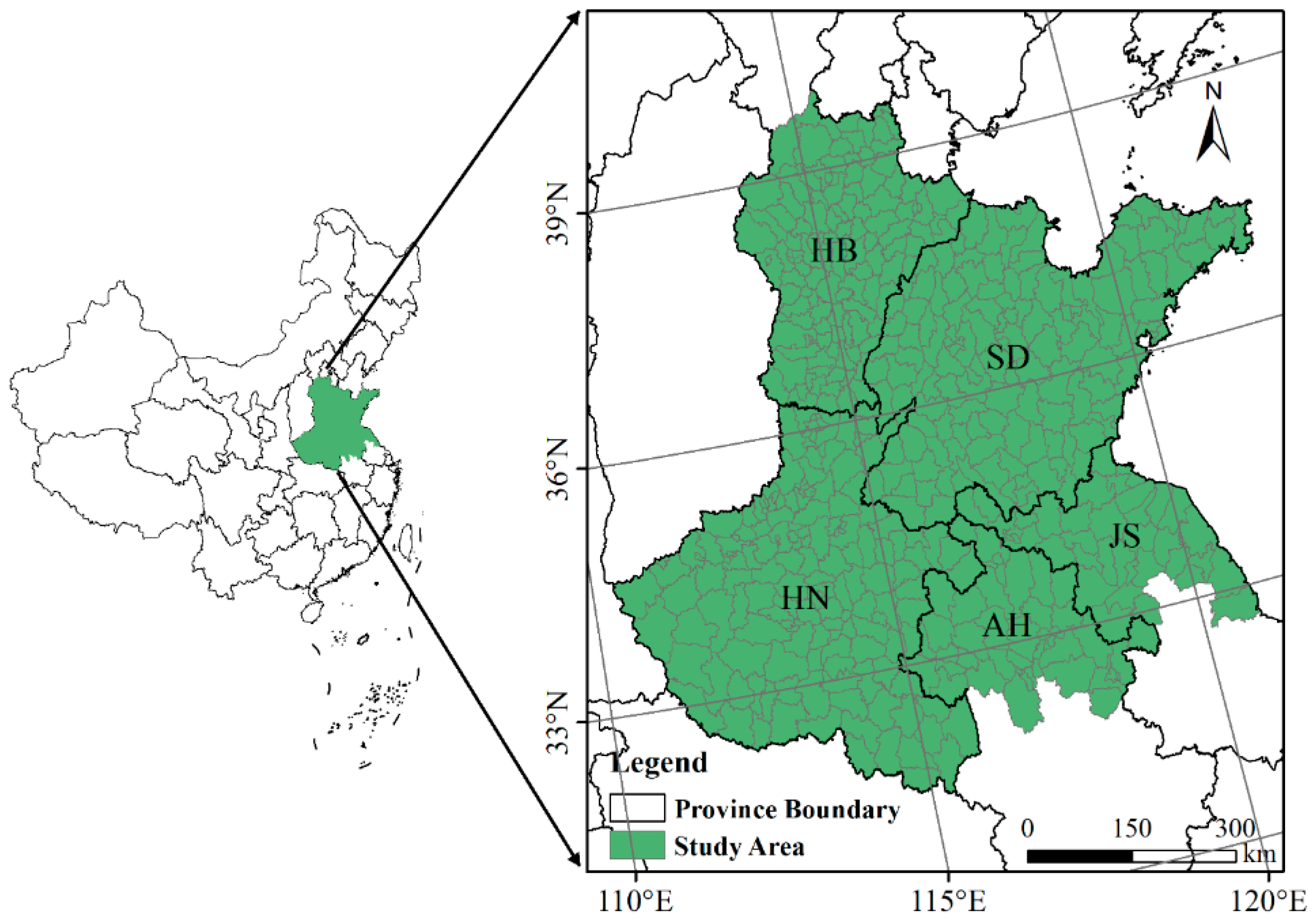
2.1. Study Area

This work focuses on the main summer maize producing region in China, the NCP, which includes most parts of Hebei (HB), Henan (HN), Shandong (SD), and the north of Jiangsu (JS) and Anhui (AH) provinces. This area of mid-eastern China, which stretches from 110°E to 122°E and from 28°N to 40°N (Figure 1), has a semi-humid monsoon climate with an annual rainfall of 400 to 800 mm (mostly falling from July to August, concentrated in the maize-growing season), and average annual temperatures that range from 10 °C in the northern part to 15 °C in the southern part of the region. The plain, where the growing season for maize runs from June to September, is one of the important grain baskets in China, producing one-third of China’s maize. Winter wheat and summer corn are rotated as the primary agricultural practice.

2.2. Datasets and Preprocessing

First, we collected data on maize growth and development from monitoring stations in Fengqiu, Yucheng, and Luancheng from 2004 to 2019 (chinaFLUX). In the NCP, the maize emergence period is primarily around mid-to-late June, and the harvest period is in late September. We concentrated on this time period in our investigation. In this study, data on maize, satellite data, and climatic data were employed.

2.2.1. Maize-Related Data

The statistical data for the county-level maize yields (measured in kg/ha), utilized in this study, were taken from the Agricultural Yearbook (stats.gov.cn, accessed on 30 October 2022) and covered the years 2000 to 2019 (a few counties have data gaps of a year or more). The following values were deemed outliers: (1) values beyond the range of biophysically viable yields; (2) values from between 2000 and 2019 that were two standard deviations above or below the mean [36,37]. If a value is missing from a time series and only one value is missing, the average of the two years before and after is used to fill in the gap; if there are two consecutive missing years, the most recent year’s data is used; and if missing for three consecutive years, the data is deemed to be missing. To predict crop yields, it is also critical to accurately identify the planting area. The planting area’s dynamic change was considered. From 2000 to 2019, China’s annual maize planting pixels at 1 km resolution, from Luo et al. [38], were utilized for mask generation.

2.2.2. Satellite Data

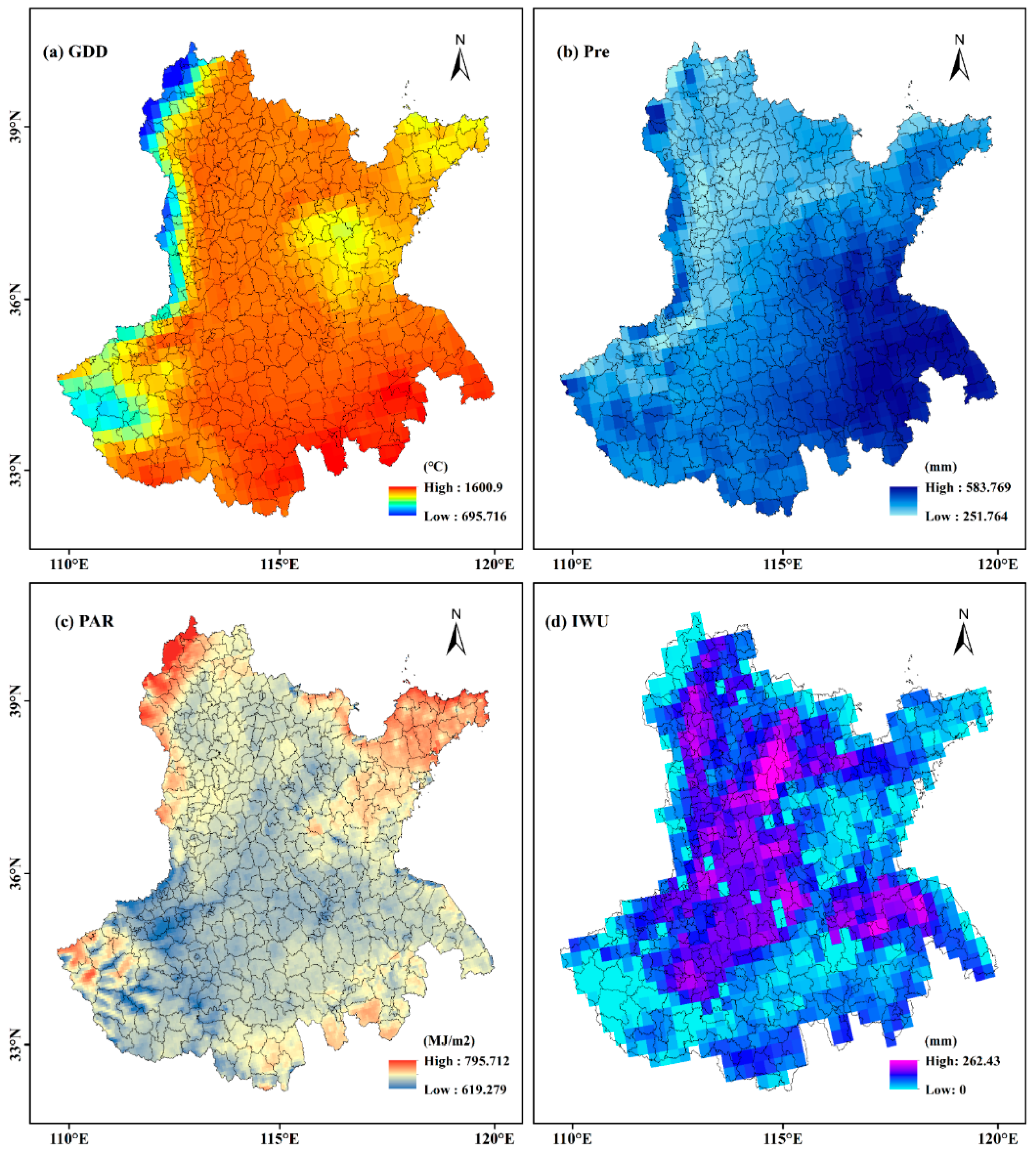
The VI for the growing season is closely related to photosynthesis and the biomass of crops. We obtained the MODIS NDVI data from the GEE platform, using the latest version (Collection 6.1), for the summer maize-growing season, from 2000 to 2019. The Savitzky–Golay (S-G) filter, which has the potential to remove random noise, was used to smooth the NDVI series in accordance with the “Quality reliability of VI pixels” metric, which describes the quality of the pixels in the data. Then, the high-quality pixels from the original sequence were used to replace the pixels at corresponding locations in the new sequence [39]. To calculate the vapor pressure deficit (VPD), we also downloaded the DEM data (digital elevation model), with a 90 m × 90 m spatial resolution, from the SRTM digital elevation dataset (http://srtm.csi.cgiar.org, accessed on 30 October 2022).

2.2.3. Climate Data

In this work, we mainly used three kinds of meteorological data, including air temperature (T), dew-point temperature (Td), and photosynthetically active radiation (PAR), which were all downloaded from the GEE platform. The daily PAR from 2000–2019, with a resolution of 0.05° × 0.05°, was derived from the BESS (Breathing Earth System Simulator) product. This product’s data exhibits a robust linear relationship with in situ measurements (R² = 0.94, and the relative bias = 1.7% for PAR) [40]. The air temperature and dew-point temperature, with a resolution of 0.1° × 0.1°, were derived from ERA-5. The VPD was calculated using the T and Td according to Yuan et al. [41]. To keep the same resolution as the NDVI, the climatic data were resampled to 1 km, and a 16-day average was calculated over the same time frame as the NDVI.

2.3. Methodology

The ecosystem’s source of both material and energy is the GPP that plants make during photosynthesis. The final crop yield is directly correlated with the amount of GPP accumulated over the course of crop growth and development. The accumulated GPP of summer maize over the study area was calculated using the EC-LUE model [42]. Then, the GPP was transformed into yield by using the HI.

2.3.1. EC-LUE Model

The model’s input data also includes the vegetation index (NDVI), which describes the biophysical characteristics of the crops, and environmental–meteorological data (including PAR, T, and Td). The following is a detailed description of the model:

$$\mathrm{GPP}=\mathrm{PAR}\times \mathrm{fPAR}\times {\epsilon }_{\max }\times \min ({\mathrm{T}}_{\mathrm{s}},{\mathrm{W}}_{\mathrm{s}})$$

(1)

$$\mathrm{fPAR}=1.24\times \mathrm{NDVI}-0.168$$

(2)

$${\mathrm{T}}_{\mathrm{S}}=\frac{(\mathrm{T}-{\mathrm{T}}_{\min })\times (\mathrm{T}-{\mathrm{T}}_{\max })}{(\mathrm{T}-{\mathrm{T}}_{\min })\times (\mathrm{T}-{\mathrm{T}}_{\max })-{(\mathrm{T}-{\mathrm{T}}_{\mathrm{opt}})}^2}$$

(3)

$$W_S=\frac{{\mathrm{VPD}}_{\max }-\mathrm{VPD}}{{\mathrm{VPD}}_{\max }-{\mathrm{VPD}}_{\min }}$$

(4)

where $\mathrm{fPAR}$ is the fraction of incident of the PAR intercepted by the crop, which has a suitable connection with the NDVI; ${\epsilon }_{\max }$ (2.84 g C m⁻² MJ⁻¹ APAR) [43] represents the light use efficiency under optimum growing conditions; and $\min ({\mathrm{T}}_{\mathrm{s}},{\mathrm{W}}_{\mathrm{s}})$ represents the minimum value between ${\mathrm{T}}_{\mathrm{s}}$ and ${\mathrm{W}}_{\mathrm{s}}$. ${\mathrm{T}}_{\mathrm{s}}$ and ${\mathrm{W}}_{\mathrm{s}}$ indicate the limitation of the temperature and water to photosynthesis, varying between 0–1. The most stressed component determines the final limit in the model. For maize photosynthetic activity, the ${\mathrm{T}}_{\min }$, ${\mathrm{T}}_{\max }$, and ${\mathrm{T}}_{\mathrm{opt}}$ were adjusted to 0 °C, 45 °C, and 23 °C, respectively, as the minimum, maximum, and optimal air temperatures [44]. When the temperature exceeds the minimum and maximum temperature range, ${\mathrm{T}}_{\mathrm{s}}$ is set to 0 [45]. The values of ${\mathrm{VPD}}_{\min }$ and ${\mathrm{VPD}}_{\max }$ are 650 Pa and 4300 Pa, respectively, and they reflect the minimum and maximum values of the VPD. If the VPD is greater than ${\mathrm{VPD}}_{\max }$, ${\mathrm{W}}_{\mathrm{s}}$ is set to 0, and if the VPD is less than ${\mathrm{VPD}}_{\min }$, it is set to 1 [46].

2.3.2. Yield Estimation

We converted the GPP to crop yield using the following relationship:

$$\mathrm{Yield}=\mathrm{GPP}\times \mathrm{AR}\times \alpha \times \frac{1}{1+\mathrm{RS}}\times \mathrm{HI}\times \frac{1}{1-\mathrm{MC}}$$

(5)

where Yield is the estimated maize yield in an administrative area. GPP represents the average of the accumulated GPP over an administrative area in the summer maize growth stage. AR indicates the fraction of the GPP remaining after autotrophic respiration, which is set to 0.53, according to Waring et al. [47]. RS is the root-to-shoot ratio with a value of 0.18 [48], which was used to obtain the above-ground biomass. MC, the grain’s moisture content at harvest, has a value of 0.11 for maize [49]. HI represents the harvest index, measuring the percentage of the above-ground biomass that is converted to economic yield. Moreover, α, with a value of 2.22, is the conversion factor of carbon content to dry matter [50].

2.3.3. Calibration of the Harvest Index

The HI, which represents the percentage of above-ground biomass that is converted to economic yield and indicates the percentage of the biomass allocated to harvesting organs, is a significant factor influencing crop yield. Numerous elements, including cultivars, management, and growing circumstances, might affect the HI. In order to take into consideration the temporal and spatial volatility of the HI, we referred back to the method used by Ju et al. [51] to calculate the HI for each county based on the estimated GPP and statistical yield in the prior year. Then, the calibrated HI was used to convert the GPP estimated by the model into the crop yield for the year. For the counties where the HI was missing, we used the HI mean from the neighboring counties instead.

2.4. Model Accuracy Evaluation and Validation

To assess the estimated maize yield, we computed the coefficient of determination (R²), root mean square error (RMSE), mean absolute percentage error (MAPE) and the revised Willmott’s index of agreement (${\mathrm{d}}_{\mathrm{r}}$) [52]. The general rule is that the higher the R², the lower the RMSE, signifying a higher accuracy of the estimated yield, and the lower the MAPE, the smaller the difference between the estimated yield and the statistical yield. The ${\mathrm{d}}_{\mathrm{r}}$ is a good indicator to evaluate the model performance, especially relative to the 1:1 best-fit line, and the ${\mathrm{d}}_{\mathrm{r}}$ provides information about the predicted and observed values on the deviation from the observed mean [53,54]. The following calculation formula is used:

$$\mathrm{RMSE}=\sqrt{\frac{1}{\mathrm{n}}{\displaystyle \sum _{\mathrm{i}=1}^{\mathrm{n}}{({\mathrm{Y}}_{\mathrm{i}}-{\mathrm{X}}_{\mathrm{i}})}^2}}$$

(6)

$$\mathrm{MAPE}=\frac{1}{\mathrm{n}}{\displaystyle \sum _{\mathrm{i}=1}^{\mathrm{n}}\left|\frac{{\mathrm{Y}}_{\mathrm{i}}-{\mathrm{X}}_{\mathrm{i}}}{{\mathrm{X}}_{\mathrm{i}}}\right|}\times 100$$

(7)

$${\mathrm{d}}_{\mathrm{r}}=\left\{\begin{array}{l}1-\frac{{\displaystyle {\sum }_{\mathrm{i}=1}^{\mathrm{n}}|{\mathrm{Y}}_{\mathrm{i}}-{\mathrm{X}}_{\mathrm{i}}|}}{\mathrm{c}{\displaystyle {\sum }_{\mathrm{i}=1}^{\mathrm{n}}|{\mathrm{X}}_{\mathrm{i}}-\overline{\mathrm{X}}|}},\mathrm{when}{\displaystyle {\sum }_{\mathrm{i}=1}^{\mathrm{n}}|{\mathrm{Y}}_{\mathrm{i}}-{\mathrm{X}}_{\mathrm{i}}|}\le \mathrm{c}{\displaystyle {\sum }_{\mathrm{i}=1}^{\mathrm{n}}|{\mathrm{X}}_{\mathrm{i}}-\overline{\mathrm{X}}|}\\ \frac{\mathrm{c}{\displaystyle {\sum }_{\mathrm{i}=1}^{\mathrm{n}}|{\mathrm{X}}_{\mathrm{i}}-\overline{\mathrm{X}}|}}{{\displaystyle {\sum }_{\mathrm{i}=1}^{\mathrm{n}}|{\mathrm{Y}}_{\mathrm{i}}-{\mathrm{X}}_{\mathrm{i}}|}}-1,\mathrm{when}{\displaystyle {\sum }_{\mathrm{i}=1}^{\mathrm{n}}|{\mathrm{Y}}_{\mathrm{i}}-{\mathrm{X}}_{\mathrm{i}}|>\mathrm{c}{\displaystyle {\sum }_{\mathrm{i}=1}^n|{\mathrm{X}}_{\mathrm{i}}-\overline{\mathrm{X}}|}}\end{array}\right.$$

(8)

where n is the number of administrative regions, ${\mathrm{Y}}_{\mathrm{i}}$ denotes the estimated yield, and ${\mathrm{X}}_{\mathrm{i}}$ denotes the statistical yield for the ith region. $\overline{\mathrm{X}}$ represents the statistical yield, on average, across all administrative regions. Moreover, ${\mathrm{d}}_{\mathrm{r}}$ has a range from −1 to 1, which implies that the model is performing better when its value is nearer 1, and c equals 2.

3. Results

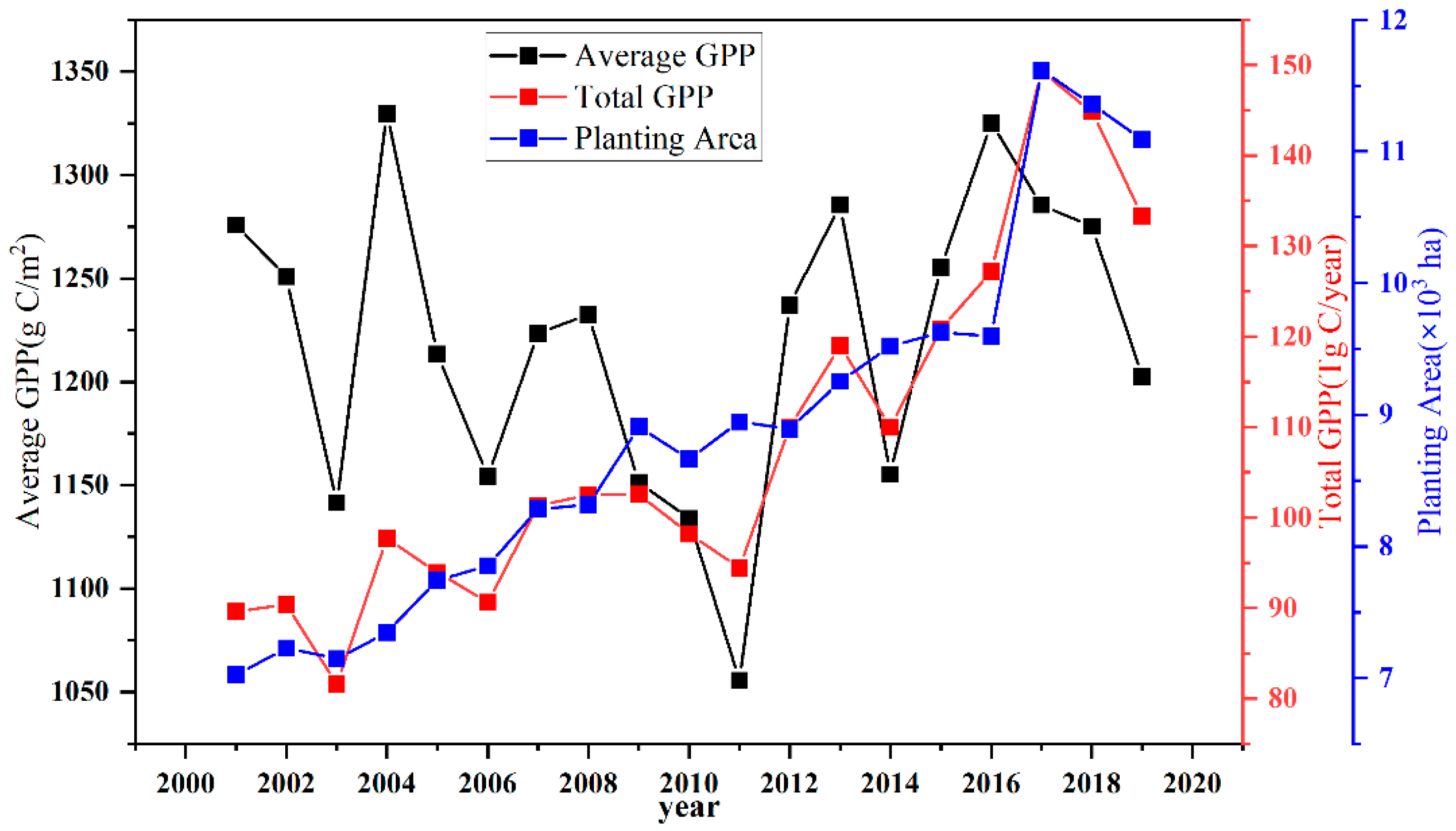
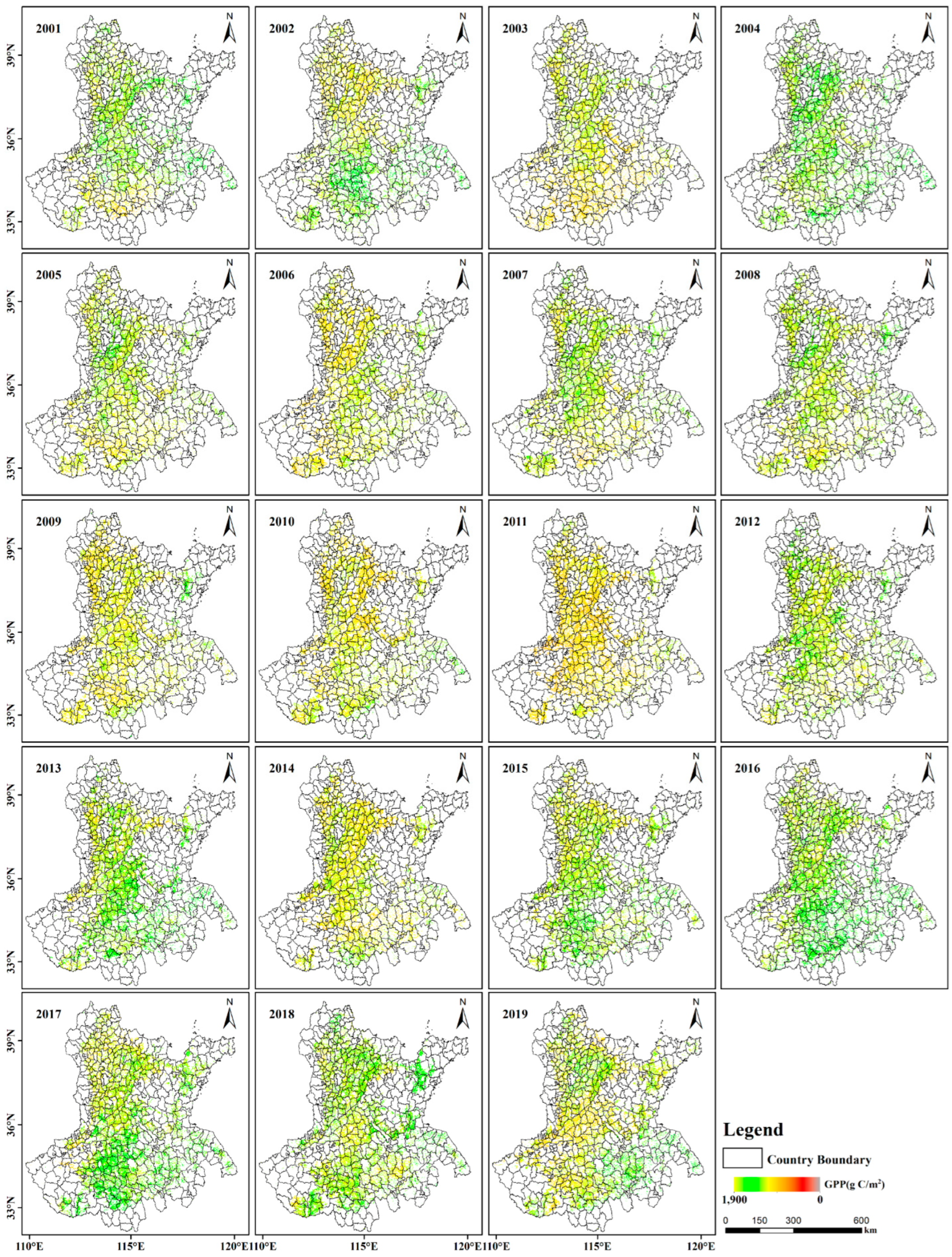
3.1. Gross Primary Productivity of Maize in the NCP

There are large spatiotemporal differences in the estimated GPP in the NCP regions. For example, in 2019, the high-value GPP zones are concentrated in the southeast of the NCP (AH and JS), with values greater than 1400 g C/m² in the majority of those regions, whereas the low-value areas are primarily located in the centre area of the NCP, with many values lower than 1000 g C/m² (Appendix A, Figure A1). The average GPP showed a declining tendency from 2001 to 2011, with a decrease of up to −15.67 ± 5.76 g C/m²/year, and an upward trend from 2011 to 2019, with an increase of 14.52 ± 10.00 g C/m²/year (Figure 2). Also shown in Figure 2 is the cumulative total GPP for the summer maize-growing season in the NCP region, which increased at an average annual growth rate of 2.30 Tg C/year, from 89.63 Tg C/year in 2001 to 133.34 Tg C/year in 2019. The increase in the total GPP is primarily due to an increase in the area planted with summer maize. Summer maize planting space increased from 7.03 × 10⁴ ha in 2001 to 11.09 × 10⁴ ha in 2019, growing at an average rate of 2.14 × 10³ ha/year.

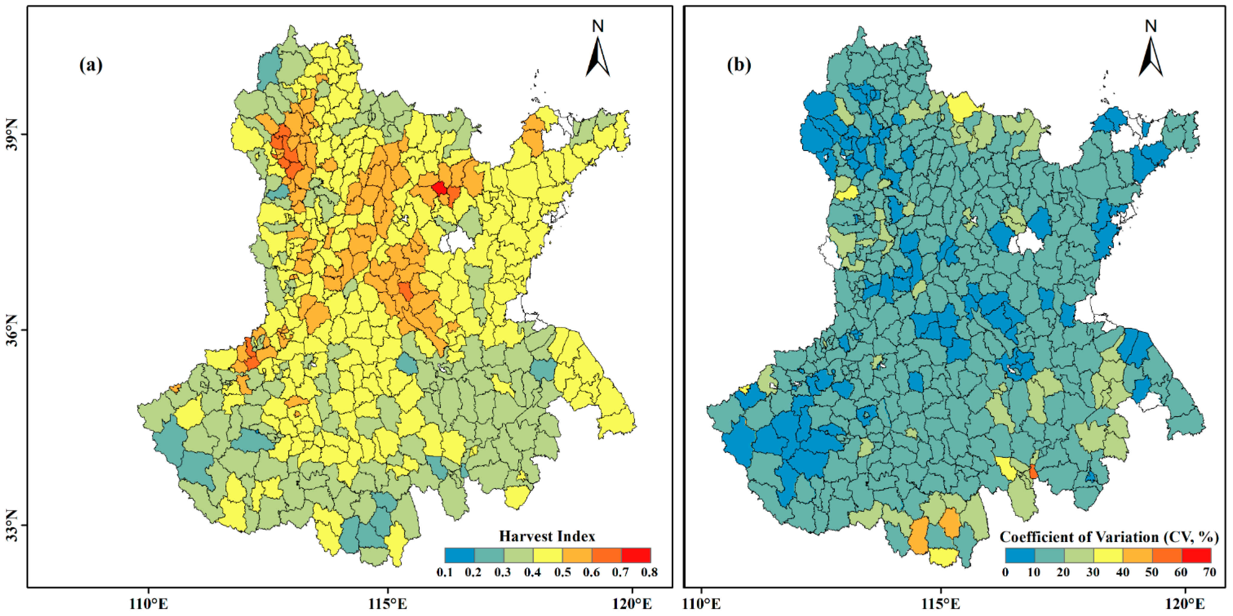
3.2. Distribution of the Harvest Index

The HI is a key parameter in the model that affects how accurately crop yield predictions are made. In this work, the HI was calibrated for each county-level district using the estimated GPP and statistical yield. Figure 3a illustrates the average HI for each county, from 2001 to 2019, demonstrating the significant regional variation in the HI. The difference between the different counties even exceeds 0.4. The HI displays the spatial characteristics, which are low in the south and high in the north. In general, HB and SD are higher than in HN, JS, and AH, and the mean values for the HI are, respectively, 0.46, 0.48, 0.41, 0.39, and 0.37. The HI distribution range consists primarily of the intervals 0.3–0.4 and 0.4–0.5, accounting for more than 77% of the total, followed by 0.5–0.6, accounting for 17.19%, and the sum of less than 0.3 and greater than 0.6 being less than 6%. The calibrated HI values in this investigation are consistent with the findings in earlier studies, proving that this approach can successfully invert the HI. For instance, the HI fluctuation range for the main maize-growing regions in China (2009–2016) was 0.25–0.67, and the values from the HI in the NCP area were 0.32–0.64, according to the field investigation by Liu et al. [55]. The corrected HI can be used to convert the GPP to maize output.

Furthermore, we explored the volatility of the HI over time. Figure 3b shows the coefficient of variation (CV) in the county-level HI from 2001 to 2019. Only a few county-level administrative regions have a CV in the HI that is greater than 20%, indicating a small degree of variation in the summer maize HI from 2001 to 2019.

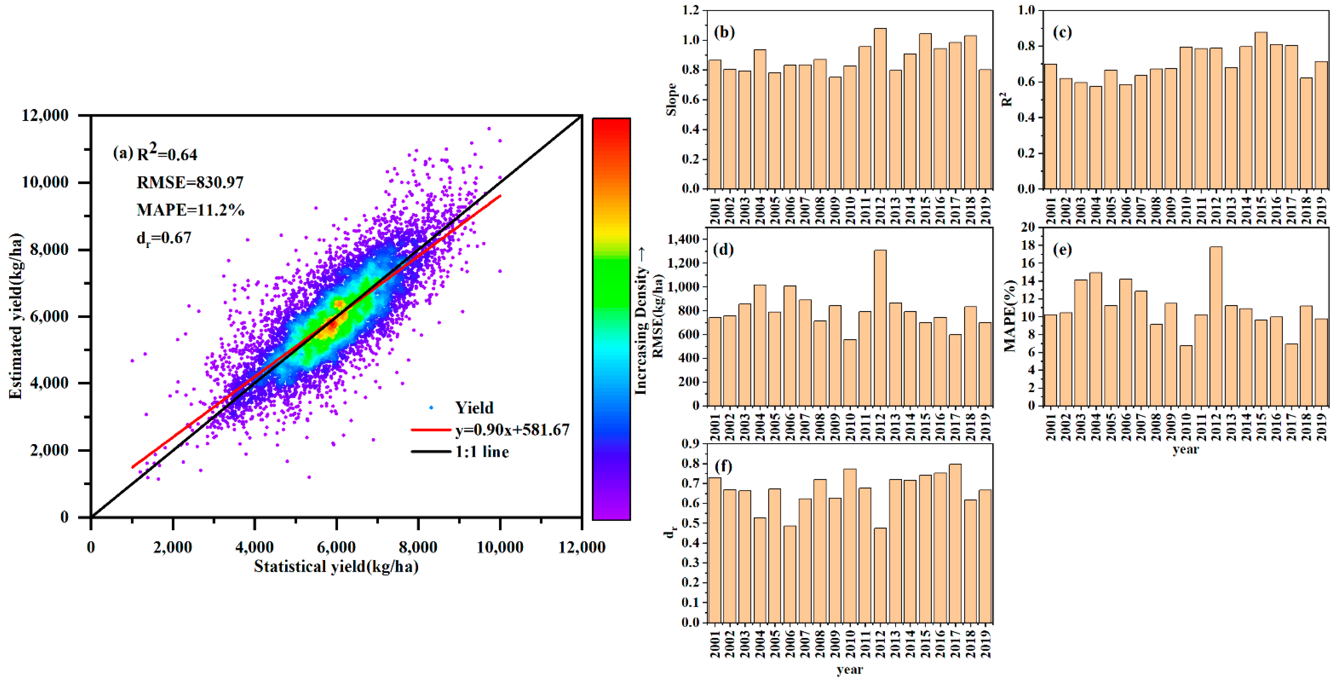
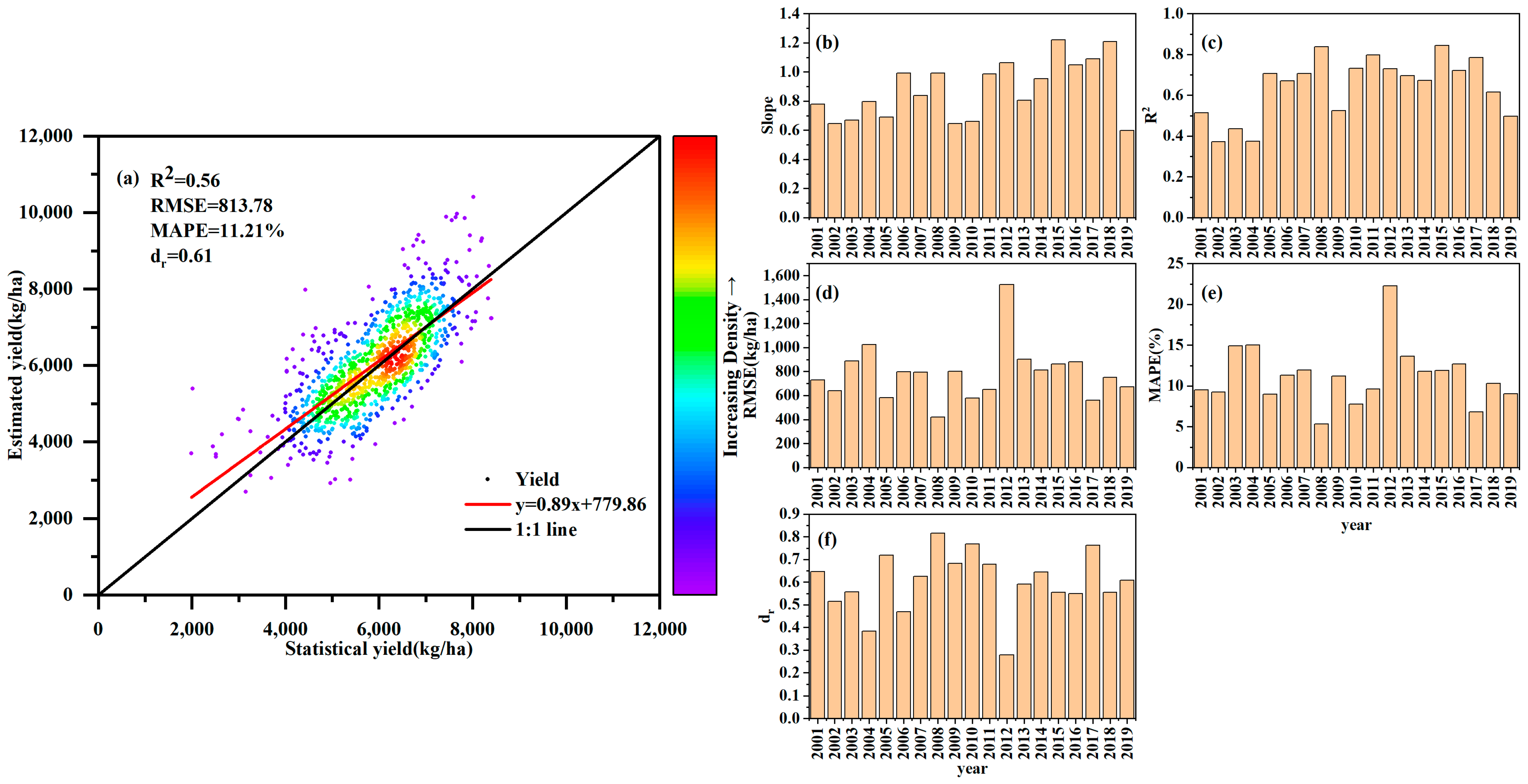
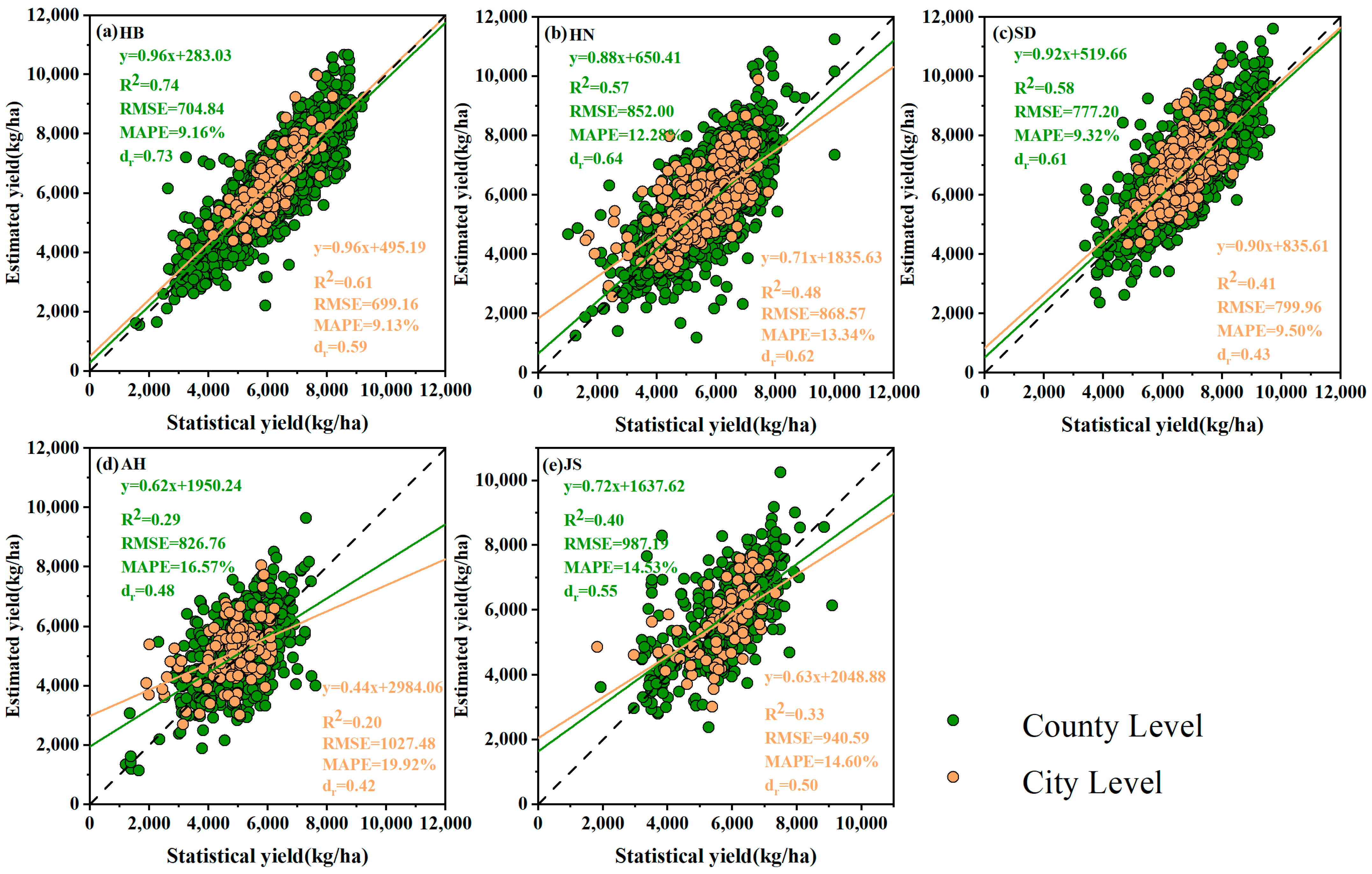
3.3. Validation of the Estimated Yield

Accuracy testing is crucial for agricultural yield estimation. We evaluated the model’s performance in estimating maize yield at the county and municipal levels based on the statistical yield.

Across all research years, the estimated yields can account for 64% of the spatiotemporal variation in yield at the county level (Figure 4a). The indicators of model performance were the RMSE, MAPE, and ${\mathrm{d}}_{\mathrm{r}}$, which were 830.97 kg/ha, 11.20%, and 0.67, respectively. Additionally, we contrasted each year’s statistical yield with the estimated yield. The linear regression slope between the statistical and estimated yield varies from 0.75 to 1.08 (Figure 4b), and the average value is 0.88, indicating a lower deviation between the two yields at the county level. The R² values are higher than 0.57 every year, the RMSE values are between 555.47 kg/ha and 1018.53 kg/ha, all of the MAPE values are below 20%, and the majority of the ${\mathrm{d}}_{\mathrm{r}}$ values are above 0.5 (Figure 4c–f). However, there are still some years where the estimated and statistical yields diverge significantly. For instance, even though the R² values are higher than 0.57 and the MPEA values are lower than 20%, the ${\mathrm{d}}_{\mathrm{r}}$ in 2006 and 2012 is only 0.48 and 0.47, respectively, indicating that these two years saw poor performance.

In addition, based on the HI calibrated at the county scale, the estimated yields and statistical yields were also contrasted at the municipal scale. On the city level, the estimated yields can account for 56% of the variation in the yield for all years (Figure 5a). The RMSE, MAPE, and ${\mathrm{d}}_{\mathrm{r}}$ were 813.78 kg/ha, 11.21% and 0.61, respectively. Additionally, we ran regression analysis for each year’s estimated and statistical yields. In general, the model predictions can also simulate how the statistical yield changes in the majority of the years. The linear regression’s slope for statistical and estimated yields ranged from 0.6 to 1.22 for all years (Figure 5b). The R² values range from 0.37 in 2002 to 0.84 in 2015. Figure 5b–e shows that the model can still estimate maize production well at the city scale. The RMSE ranges from 420.14 kg/ha (2008) to 1523.37 kg/ha (2012), the MAPE values are less than 20%, except for 2012 (22.24%), and the ${\mathrm{d}}_{\mathrm{r}}$ values are greater than 0.45, except for 2004 (0.38) and 2012 (0.28) (Figure 5c–f), which also shows that the model can still estimate the yield well at the city scale. All of these results imply that, despite its inconsistent performance in some years, the estimated yield accurately captures the changes in production over time, particularly at the county level. The model’s accuracy met the requirements for assessing regional maize yield across the NCP.

The crop output varies from region to region and is influenced by climate factors, soil characteristics, and management techniques [18]. As a result, we compared the model in different provinces to confirm how well it performed in various places. Overall, good performance was achieved in HB, HN, and SD; the R² values are 0.74, 0.57, and 0.58 at the county level and 0.61, 0.48, and 0.41 at the city level, respectively (Figure 6a–c). While it performed poorly in AH and JS, the R² are only 0.29 and 0.40 at the county level, and 0.20 and 0.33 at the city level, and all the MAPE values are larger than 14% for both levels (Figure 6d,e). There exist some differences between different provinces, and great uncertainties in the AN and JS provinces.

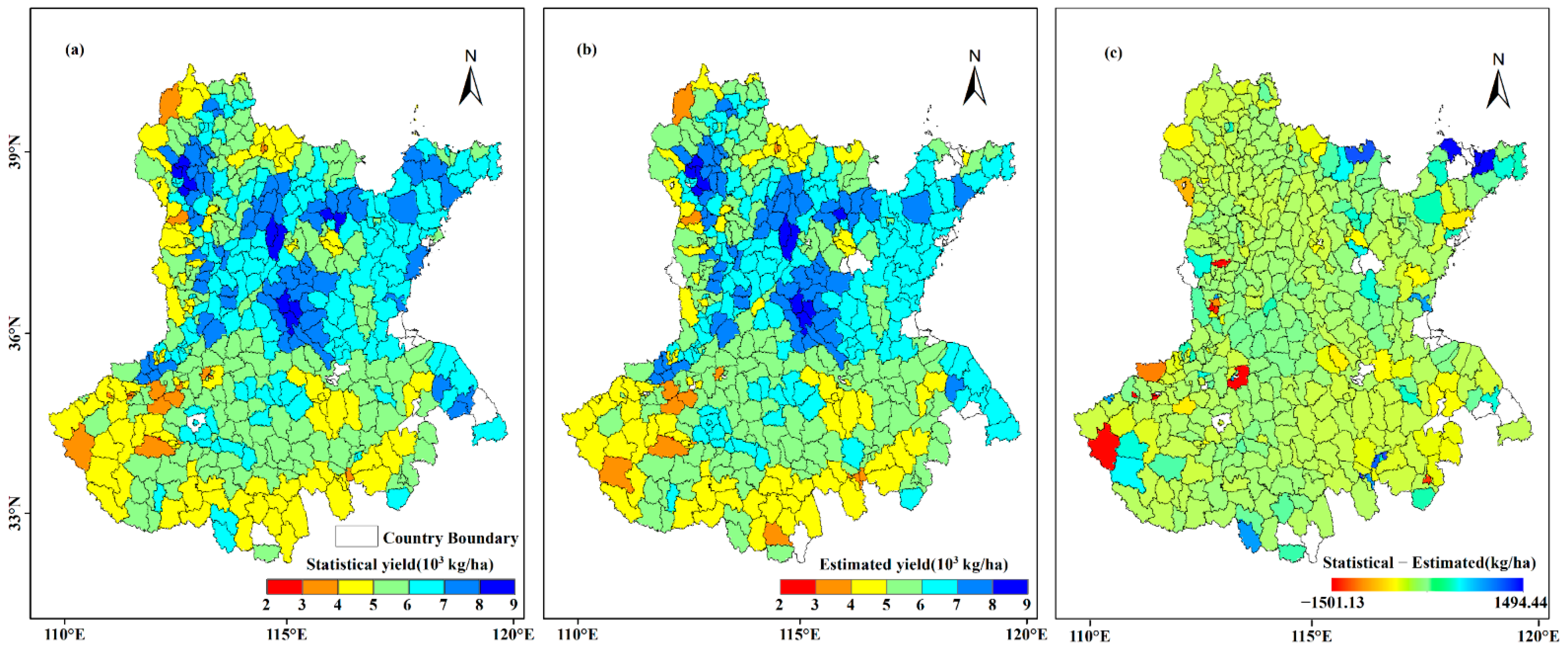
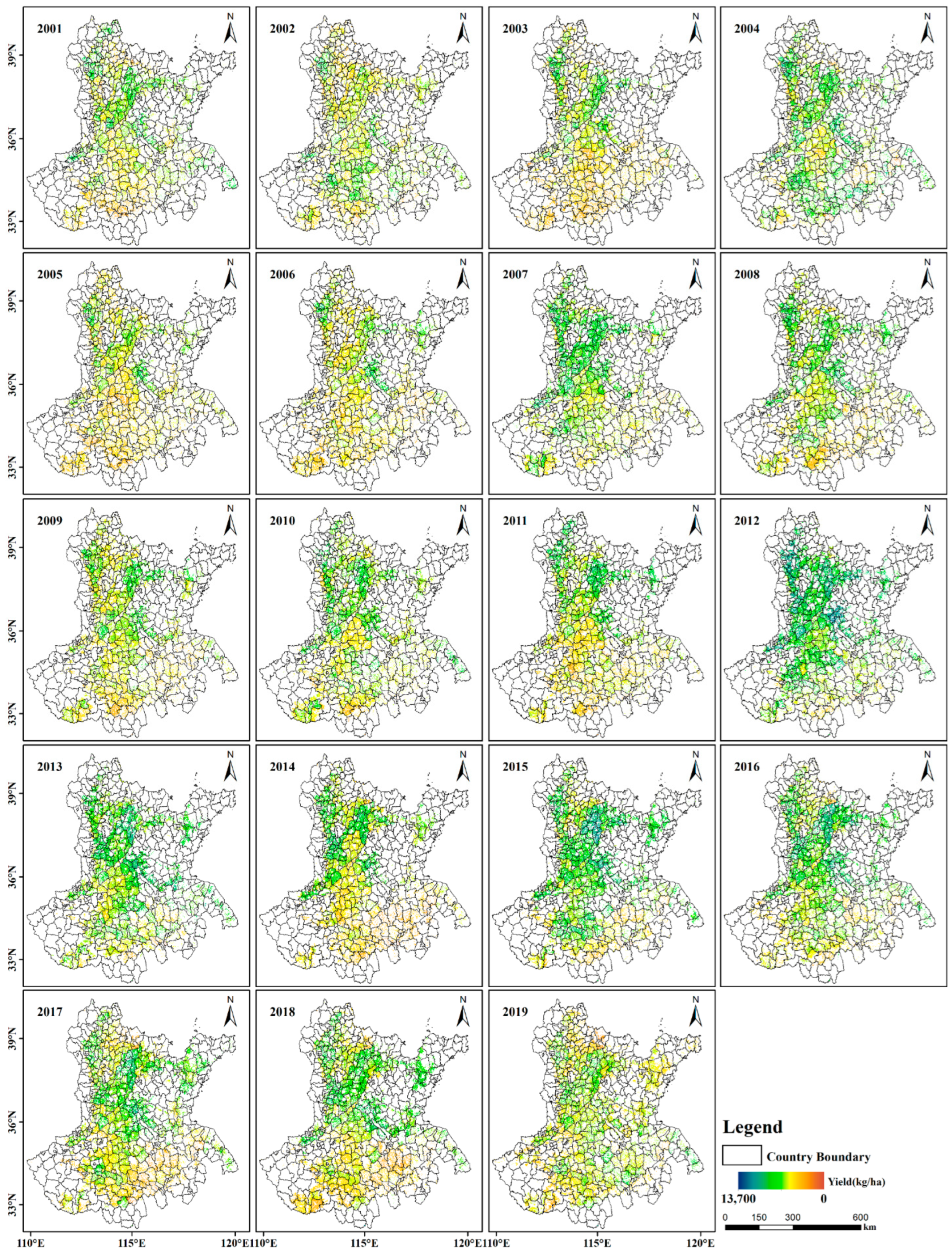
3.4. The Pattern of the Summer Maize Yield’s Spatial Distribution

In this work, we converted the estimated GPP using the LUE model to the summer maize yield based on the corrected HI. Figure A2 shows the maize yield’s spatial distribution, at the pixel scale, from 2001 to 2019. Generally, the estimated maize yield in the NCP region is mainly distributed between 5000–7000 kg/ha, accounting for 61.6%. There are a few pixels less than 1000 kg/ha or more than 11000 kg/ha. In addition, we compared the spatial distribution of the estimated and statistical yields. Figure 7a,b shows the county-level spatial distribution of the mean statistical yield and the mean estimated yield from 2001 to 2019, demonstrating good consistency between the two and the accuracy of the model’s estimated yield. The projected yields display a distribution pattern of high in the north and low in the south, similar to the statistical yields. Overall, HB and SD had greater maize mean yields than HN, AH, and JS. Moreover, they demonstrate the significant regional variation in the maize yield over the NCP. In certain areas, like Dezhou city in SD province, the maize mean yield estimations are greater than 7000 kg/ha or even exceed 8000 kg/ha, while in other areas, like the majority of the county-level administrative districts in AH and several county-level areas in western and southern HN province, they are less than 5000 kg/ha. Additionally, we subtracted the estimated yield from the statistical yield and discovered that the results were concentrated between −300 and 200 kg/ha. The difference between the statistical and estimated mean yield is particularly noticeable in areas with small and dispersed planting areas, like some counties in SD province and western HN province (Figure 7c).

We also investigated the spatial association between the yield distribution and climate factors, such as precipitation (pre), air temperature (T), and photosynthetically active radiation (PAR). Pre is mainly found in the southeast, gradually decreasing from southeast to northwest. From south to north, T declines. Although PAR is higher in the SD Peninsula, it does not vary significantly throughout the research area (Figure 8). The average maize yield’s regional distribution pattern differs from that of Pre, T, or PAR. Irrigation can be an important factor in influencing maize yields in the NCP, especially in HB and western SD provinces. From previous studies, it can be concluded that the NCP area has a high proportion of crop irrigation [56,57]. In addition, we averaged the irrigation water use data (IWU, driven by Zhang et al. [58]) during June-September from 2011 to 2018 and found that the maize yields were highly consistent with IWU in HB and western SD provinces, with a high yield in areas with high IWU and a poor yield in areas with low IWU.

4. Discussion

According to previous studies, the EC-LUE model is capable of simulating the spatiotemporal variation in winter wheat yield at the national level and has the capacity to do the same for other crop yields [35]. However, few studies have focused on maize yield. MODIS remote sensing images remain an important source of information for monitoring crop yields over large areas. In this study, maize yield in the NCP region was successfully estimated using an EC-LUE model based on MODIS vegetation index data and ERA-5 reanalysis data, indicating that the yield of different crops can be estimated using the EC-LUE model combined with the calibrated HI.

In this work, we treated the HI calibrated at the county scale as the HI for each planted cell of maize within the corresponding administrative region. In China, farmers are basic agricultural production units [59], which increases the spatial variability in the crop HI. It can be particularly difficult to directly obtain the HI per pixel on a large spatial scale, because of the lack of regional cultivar and management data. The validation results show that it is feasible to use a calibrated HI in the model. Some studies have used similar methods to calibrate the HI for yield estimation with good results [51,60]. In many crop models, such as AQUACROP [61] and CROPSYST [62], the HI is a crucial variable. Some methods for estimating the HI based on remote sensing are considered feasible in large areas. Based on fractional post-anthesis phase growth, Kemanian et al. [33] devised a straightforward method to calculate the HI, proposing that the HI was correlated with the ratio of the above-ground biomass produced following blooming with that produced throughout the entire growing season. However, this method requires a high temporal resolution in the remote sensing data in order to accurately extract the flowering period. Campoy et al. [32] used the ratio between the variables (e.g., absorbed photosynthetically active radiation, crop transpiration coefficient, and crop transpiration) related with biomass production to estimate the HI. However, the difficulty in accurately estimating the crop transpiration will lead to huge errors [35]. Although the HI estimated by remote sensing methods has high accuracy (R² values ranging from 0.69 to 0.79), further research is needed [12]. In this study, the calibrated HI for maize mainly varies between 0.2–0.6 at the county level, which is comparable to the reported values. Liu et al. [54] summarized the HI with values ranging from 0.25 to 0.67 in the main corn producing regions across China (2009–2016), and the values in the HI are between 0.32 and 0.64 in the NCP. In addition, some counties have a calibrated HI less than 0.2 or greater than 0.6, and these areas tend to have fewer maize-growing pixels. In addition, the uncertainty in the statistical yield causes errors in the calibration of the HI [63]. Furthermore, a higher cumulative GPP of maize during the growing season does not imply a higher grain yield, and there is a significant positive correlation between grain yield and the HI [64]. The regional distribution of the estimated maize yield in this study is similar to the HI. One study showed that the contribution rate of the HI (52.67%) was higher than that of dry matter (47.33%) in the NCP [54]. Although the use of the calibrated HI in the model performed well, it ignores the changes in maize varieties and cultivars. The HI differed significantly between different maize cultivars [55]. Future studies will benefit from more precise variety and yield data for yield estimation.

In addition, the crop area and NDVI have a significant impact on how accurately the GPP and yield are estimated. The crop area dataset that was employed in this study was spatially explicit and temporally continuous, which considerably reduced inaccuracies brought on by changes in maize planting areas. A pixel with a 1 km resolution may contain several different forms of land cover or crops, which might cause uncertainty in the results [65,66]. In this instance, regions with large, contiguous planting areas have smaller errors in the results, while regions with tiny, dispersed planting areas have more errors in the results. A further factor in the inaccuracy is the treatment of non-crop growing areas as crop growing areas, or crop growing areas as non-crop planting areas, due to the intricacy of the surface. In terms of the NDVI, pixels that are combined with trees will have higher values, whereas pixels that are mixed with impermeable surface or bare ground will have lower values, resulting in a higher or lower GPP for estimation. This introduces an inevitable error in the harvest index correction. This is also one of the reasons for the extremely low or extremely high values in the yield estimates. In contrast, AH and JS have smaller and more dispersed maize planting areas than HB, HN, and SD, which may be one of the causes of the inaccurate maize yield estimations in these two regions. Fortunately, we were able to preserve the original signal when reconstructing the NDVI time series using the S-G filter, allowing the NDVI series to accurately depict maize growth and development. Although Landsat and Sentinel-2 have higher spatial resolution, they are more affected by noise [67]. In order to facilitate crop production estimation using remote sensing data, more advanced processing techniques are urgently required.

Moreover, uncertainty exists in the parameters characterizing crop biophysics. A fixed value for ${\epsilon }_{\max }$, a crucial model parameter, may result in systematic uncertainty or mistakes in the GPP for dynamic simulations of a specific region [63,68]. Wagle et al. [69] demonstrated that even in the same site, the ${\epsilon }_{\max }$ changed from year to year. Although utilizing fixed efficiency values to estimate the biomass over crop growth cycles has advantages, meteorological and management conditions are nonetheless crucial determinants of their dynamic variations, according to a recent study [30]. Additionally, variable canopy structures, row spacings, and plant densities effect the ${\epsilon }_{\max }$ of maize [70,71]. Although the ${\epsilon }_{\max }$ value we used (2.84 g C m⁻² MJ⁻¹ APAR) was in the right range, GPP errors were inevitable. For the temperature, we set the suitable growing temperature for maize to 0–45 °C, which is within the reported growth temperature range. Crafts-Brandner and Salvucci [72] discovered that the ideal temperature for maize ranged from 28 °C to 37.5 °C, and that setting the ideal temperature at 23 °C can cause GPP mistakes. The three parameters (AR = 0.53, RS = 0.18, and MC = 0.11) that translate GPP into crop production still have considerable room for error. These three criteria may change based on crop cultivars and varieties, as well as environmental factors [65]. For instance, Wang et al. [73] discovered that there was significant uncertainty in the allocation of GPP with a fixed root/shoot ratio since the maize cultivar and planting year had a significant impact on the root/shoot ratio. The AR varies with the temperature and crop development stage [74]. Future efforts to accurately predict GPP and enhance yield estimates will benefit from the rigorous calibration of these parameters for particular regions. Additionally, because there are variations in cultivation seasons, particularly in regions where farmers are the primary unit of production, using a set summer maize-growing period across the whole research area creates errors [75]. Therefore, it is noteworthy that thorough crop phenology enables more precise production estimations to be made on a broader scale [14,21,38].

5. Conclusions

In this study, the EC-LUE model was used to estimate the cumulative values on the gross primary productivity of maize during the growing season in the NCP from 2000 to 2019, based on satellite data and meteorological analysis data. The county-level HI was calibrated by combining the GPP and statistical yield. Then, the GPP was converted into the yield by using the calibrated HI. To evaluate the accuracy of the estimated yield, we compared the estimates and statistics on the county and city scales. The results show that the average growth rate in the total GPP in the summer maize-growing season from 2001 to 2019 was 2.30 Tg C/year, which was directly related to the increase in planting area. The HI has significant heterogeneity in space and little fluctuation in time between 2001 and 2019. Our estimated yield can simulate 64% and 55% of the yield variability on the county and city scale, respectively, and the model captures accurately the inter-annual changes in the maize yield. The county-level and city-level linear regression slopes vary between 0.75–1.08 and 0.6–1.22, respectively, and the MAPE is less than 20% in almost all years for both scales. But the model performance varies from region to region, HB (R² = 0.74), HN (R² = 0.57), and SD (R² = 0.58) outperformed AH (R² = 0.29) and JS (R² = 0.40) in terms of performance. That is especially true because the combination of the model and the calibrated HI enables estimates on the maize yields from county to province, and for even larger areas. Our study demonstrates that the EC-LUE model can be used to estimate maize yield and highlights the importance of employing a dynamic HI. This study can be considered as a complement to previous studies, demonstrating that the EC-LUE model can be applied to the large-scale estimation of crop yields for various crops, and can contribute to regional and national food production security.

References

1. Wang, Y.; Gong, Y. Spectral Remote Sensing Technology Applied in Crop Yield Estimation: Research Progress. Chin. Agric. Sci. Bull. 2019, 35, 69–75. [Google Scholar]
2. López-Lozano, R.; Baruth, B. An Evaluation Framework to Build a Cost-Efficient Crop Monitoring System. Experiences from the Extension of the European Crop Monitoring System. Agric. Syst. 2019, 168, 231–246. [Google Scholar] [CrossRef]
3. FAO. Fao’s Director-General on How to Feed the World in 2050. Popul. Dev. Rev. 2009, 35, 837–839. [Google Scholar] [CrossRef]
4. Zampieri, M.; Ceglar, A.; Dentener, F.; Dosio, A.; Naumann, G.; van den Berg, M.; Toreti, A. When Will Current Climate Extremes Affecting Maize Production Become the Norm? Earth’s Future 2019, 7, 113–122. [Google Scholar] [CrossRef]
5. Wang, Y.; Xu, X.; Huang, L.; Yang, G.; Fan, L.; Wei, P.; Chen, G. An Improved CASA Model for Estimating Winter Wheat Yield from Remote Sensing Images. Remote Sens. 2019, 11, 1088. [Google Scholar] [CrossRef]
6. Rosenzweig, C.; Elliott, J.; Deryng, D.; Ruane, A.C.; Müller, C.; Arneth, A.; Boote, K.J.; Folberth, C.; Glotter, M.; Khabarov, N.; et al. Assessing Agricultural Risks of Climate Change in the 21st Century in a Global Gridded Crop Model Intercomparison. Proc. Natl. Acad. Sci. USA 2014, 111, 3268–3273. [Google Scholar] [CrossRef]
7. Ren, J.; Chen, Z.X.; Zhou, Q.B.; Liu, J.; Tang, H. MODIS Vegetation Index Data Used for Estimating Corn Yield in USA. J. Remote Sens. 2015, 19, 568–577. [Google Scholar]
8. Fang, H.; Liang, S.; Hoogenboom, G.; Teasdale, J.; Cavigelli, M. Corn-Yield Estimation through Assimilation of Remotely Sensed Data into the CSM-CERES-Maize Model. Int. J. Remote Sens. 2008, 29, 3011–3032. [Google Scholar] [CrossRef]
9. Lobell, D.B. The Use of Satellite Data for Crop Yield Gap Analysis. Field Crops Res. 2013, 143, 56–64. [Google Scholar] [CrossRef]
10. Li, Z.; Taylor, J.; Yang, H.; Casa, R.; Jin, X.; Li, Z.; Song, X.; Yang, G. Field Crops Research A Hierarchical Interannual Wheat Yield and Grain Protein Prediction Model Using Spectral Vegetative Indices and Meteorological Data. Field Crops Res. 2019, 248, 107711. [Google Scholar] [CrossRef]
11. Zhang, J.; Feng, L.; Yao, F. Improved Maize Cultivated Area Estimation over a Large Scale Combining MODIS-EVI Time Series Data and Crop Phenological Information. ISPRS J. Photogramm. Remote Sens. 2014, 94, 102–113. [Google Scholar] [CrossRef]
12. Wu, B.; Zhang, M.; Zeng, H.; Tian, F.; Potgieter, A.B.; Qin, X.; Yan, N.; Chang, S.; Zhao, Y.; Dong, Q.; et al. Challenges and Opportunities in Remote Sensing-Based Crop Monitoring: A Review. Natl. Sci. Rev. 2022, 10, nwac290. [Google Scholar] [CrossRef]
13. Zhang, X.; Zhang, Q. Monitoring Interannual Variation in Global Crop Yield Using Long-Term AVHRR and MODIS Observations. ISPRS J. Photogramm. Remote Sens. 2016, 114, 191–205. [Google Scholar] [CrossRef]
14. Dong, J.; Lu, H.; Wang, Y.; Ye, T.; Yuan, W. Estimating Winter Wheat Yield Based on a Light Use Efficiency Model and Wheat Variety Data. ISPRS J. Photogramm. Remote Sens. 2020, 160, 18–32. [Google Scholar] [CrossRef]
15. Qader, S.H.; Dash, J.; Atkinson, P.M. Forecasting Wheat and Barley Crop Production in Arid and Semi-Arid Regions Using Remotely Sensed Primary Productivity and Crop Phenology: A Case Study in Iraq. Sci. Total Environ. 2018, 613, 250–262. [Google Scholar] [CrossRef]
16. Cao, J.; Zhang, Z.; Tao, F.; Zhang, L.; Luo, Y.; Han, J.; Li, Z. Identifying the Contributions of Multi-Source Data for Winter Wheat Yield Prediction in China. Remote Sens. 2020, 12, 750. [Google Scholar] [CrossRef]
17. Cheng, Z.; Meng, J.; Wang, Y. Improving Spring Maize Yield Estimation at Field Scale by Assimilating Time-Series HJ-1 CCD Data into the WOFOST Model Using a New Method with Fast Algorithms. Remote Sens. 2016, 8, 303. [Google Scholar] [CrossRef]
18. Zhang, Y.; Wang, L.; Chen, X.; Liu, Y.; Wang, S.; Wang, L. Prediction of Winter Wheat Yield at County Level in China Using Ensemble Learning. Prog. Phys. Geogr. Earth Environ. 2022, 46, 676–696. [Google Scholar] [CrossRef]
19. Han, J.; Zhang, Z.; Cao, J.; Luo, Y.; Zhang, L.; Li, Z.; Zhang, J. Prediction of Winter Wheat Yield Based on Multi-Source Data and Machine Learning in China. Remote Sens. 2020, 12, 236. [Google Scholar] [CrossRef]
20. Kang, Y.; Ozdogan, M.; Zhu, X.; Ye, Z.; Hain, C.; Anderson, M. Comparative Assessment of Environmental Variables and Machine Learning Algorithms for Maize Yield Prediction in the US Midwest. Environ. Res. Lett. 2020, 15, 064005. [Google Scholar] [CrossRef]
21. Chen, X.; Feng, L.; Yao, R.; Wu, X.; Sun, J.; Gong, W. Prediction of Maize Yield at the City Level in China Using Multi-Source Data. Remote Sens. 2021, 13, 146. [Google Scholar] [CrossRef]
22. Cao, J.; Zhang, Z.; Tao, F.; Zhang, L.; Luo, Y.; Zhang, J.; Han, J.; Xie, J. Integrating Multi-Source Data for Rice Yield Prediction across China Using Machine Learning and Deep Learning Approaches. Agric. For. Meteorol. 2021, 297, 108275. [Google Scholar] [CrossRef]
23. Filippi, P.; Jones, E.J.; Wimalathunge, N.S.; Somarathna, P.D.S.N.; Pozza, L.E.; Ugbaje, S.U.; Jephcott, T.G.; Paterson, S.E.; Whelan, B.M.; Bishop, T.F.A. An Approach to Forecast Grain Crop Yield Using Multi-Layered, Multi-Farm Data Sets and Machine Learning. Precis. Agric. 2019, 20, 1015–1029. [Google Scholar] [CrossRef]
24. Burke, M.; Lobell, D.B. Satellite-Based Assessment of Yield Variation and Its Determinants in Smallholder African Systems. Proc. Natl. Acad. Sci. USA 2017, 114, 2189–2194. [Google Scholar] [CrossRef]
25. Monteith, J.L. Solar Radiation and Productivity in Tropical Ecosystems. J. Appl. Ecol. 1972, 9, 747. [Google Scholar] [CrossRef]
26. Zhang, Y.; Xiao, X.; Wu, X.; Zhou, S.; Zhang, G.; Qin, Y.; Dong, J. A Global Moderate Resolution Dataset of Gross Primary Production of Vegetation for 2000–2016. Sci. Data 2017, 4, 170165. [Google Scholar] [CrossRef]
27. Zheng, Y.; Shen, R.; Wang, Y.; Li, X.; Liu, S.; Liang, S.; Chen, J.M.; Ju, W.; Zhang, L.; Yuan, W. Improved Estimate of Global Gross Primary Production for Reproducing Its Long-Term Variation, 1982–2017. Earth Syst. Sci. Data. 2020, 12, 2725–2746. [Google Scholar] [CrossRef]
28. Lobell, D.B.; Ortiz-Monasterio, J.I.; Falcon, W.P. Yield Uncertainty at the Field Scale Evaluated with Multi-Year Satellite Data. Agric. Syst. 2007, 92, 76–90. [Google Scholar] [CrossRef]
29. He, M.; Kimball, J.S.; Maneta, M.P.; Maxwell, B.D.; Moreno, A.; Beguería, S.; Wu, X. Regional Crop Gross Primary Productivity and Yield Estimation Using Fused Landsat-MODIS Data. Remote Sens. 2018, 10, 372. [Google Scholar] [CrossRef]
30. Campoy, J.; Campos, I.; Villodre, J.; Bodas, V.; Osann, A.; Calera, A. Remote Sensing-Based Crop Yield Model at Field and within-Field Scales in Wheat and Barley Crops. Eur. J. Agron. 2023, 143, 126720. [Google Scholar] [CrossRef]
31. HAY, R.K.M. Harvest Index: A Review of Its Use in Plant Breeding and Crop Physiology. Ann. Appl. Biol. 1995, 126, 197–216. [Google Scholar] [CrossRef]
32. Campoy, J.; Campos, I.; Plaza, C.; Calera, M.; Bodas, V.; Calera, A. Estimation of Harvest Index in Wheat Crops Using a Remote Sensing-Based Approach. Field Crops Res. 2020, 256, 107910. [Google Scholar] [CrossRef]
33. Kemanian, A.R.; Stöckle, C.O.; Huggins, D.R.; Viega, L.M. A Simple Method to Estimate Harvest Index in Grain Crops. Field Crops Res. 2007, 103, 208–216. [Google Scholar] [CrossRef]
34. Samarasinghe, G.B. Growth and Yields of Sri Lanka’s Major Crops Interpreted from Public Domain Satellites. Agric. Water Manag. 2003, 58, 145–157. [Google Scholar] [CrossRef]
35. Fu, Y.; Huang, J.; Shen, Y.; Liu, S.; Huang, Y.; Dong, J.; Han, W.; Ye, T.; Zhao, W.; Yuan, W. A Satellite-Based Method for National Winter Wheat Yield Estimating in China. Remote Sens. 2021, 13, 4680. [Google Scholar] [CrossRef]
36. Cheng, M.; Penuelas, J.; Mccabe, M.F.; Atzberger, C.; Jiao, X.; Wu, W.; Jin, X. Agricultural and Forest Meteorology Combining Multi-Indicators with Machine-Learning Algorithms for Maize Yield Early Prediction at the County-Level in China. Agric. For. Meteorol. 2022, 323, 109057. [Google Scholar] [CrossRef]
37. Cao, J.; Zhang, Z.; Luo, Y.; Zhang, L.; Zhang, J.; Li, Z.; Tao, F. Wheat Yield Predictions at a County and Field Scale with Deep Learning, Machine Learning, and Google Earth Engine. Eur. J. Agron. 2021, 123, 126204. [Google Scholar] [CrossRef]
38. Luo, Y.; Zhang, Z.; Chen, Y.; Li, Z.; Tao, F. ChinaCropPhen1km: A High-Resolution Crop Phenological Dataset for Three Staple Crops in China during 2000-2015 Based on Leaf Area Index (LAI) Products. Earth Syst. Sci. Data. 2020, 12, 197–214. [Google Scholar] [CrossRef]
39. Yin, L.; Wang, X.; Feng, X.; Fu, B.; Chen, Y. A Comparison of SSEBop-Model-Based Evapotranspiration with Eight Evapotranspiration Products in the Yellow River Basin, China. Remote Sens. 2020, 12, 2528. [Google Scholar] [CrossRef]
40. Ryu, Y.; Jiang, C.; Kobayashi, H.; Detto, M. MODIS-Derived Global Land Products of Shortwave Radiation and Diffuse and Total Photosynthetically Active Radiation at 5 Km Resolution from 2000. Remote Sens. Environ. 2018, 204, 812–825. [Google Scholar] [CrossRef]
41. Yuan, W.; Zheng, Y.; Piao, S.; Ciais, P.; Lombardozzi, D.; Wang, Y.; Ryu, Y.; Chen, G.; Dong, W.; Hu, Z.; et al. Increased Atmospheric Vapor Pressure Deficit Reduces Global Vegetation Growth. Sci. Adv. 2019, 5, eaax1396. [Google Scholar] [CrossRef]
42. Yuan, W.; Liu, S.; Zhou, G.; Zhou, G.; Tieszen, L.L.; Baldocchi, D.; Bernhofer, C.; Gholz, H.; Goldstein, A.H.; Goulden, M.L.; et al. Deriving a Light Use Efficiency Model from Eddy Covariance Flux Data for Predicting Daily Gross Primary Production across Biomes. Agric. For. Meteorol. 2007, 143, 189–207. [Google Scholar] [CrossRef]
43. Yuan, W.; Chen, Y.; Xia, J.; Dong, W.; Magliulo, V.; Moors, E.; Olesen, J.E.; Zhang, H. Estimating Crop Yield Using a Satellite-Based Light Use Efficiency Model. Ecol. Indic. 2015, 60, 702–709. [Google Scholar] [CrossRef]
44. Xie, W.; Wang, H.; Chi, H.; Dang, H.; Huang, D.; Li, H.; Cai, G.; Xiao, X. Spatial-Temporal Variation of Satellite-Based Gross Primary Production Estimation in Wheat-Maize Rotation Area during 2000–2015. Geocarto Int. 2022, 37, 2506–2523. [Google Scholar] [CrossRef]
45. Yan, H.; Fu, Y.; Xiao, X.; Huang, H.Q.; He, H.; Ediger, L. Modeling Gross Primary Productivity for Winter Wheat-Maize Double Cropping System Using MODIS Time Series and CO2 Eddy Flux Tower Data. Agric. Ecosyst. Environ. 2009, 129, 391–400. [Google Scholar] [CrossRef]
46. Running, S.W.; Zhao, M. Daily GPP and Annual NPP (MOD17A2/A3) Products NASA Earth Observing System MODIS Land Algorithm (User’s Guide V3). User Guid. 2015, 28, 1–6. [Google Scholar]
47. Waring, R.H.; Landsberg, J.J.; Williams, M. Net Primary Production of Forests: A Constant Fraction of Gross Primary Production? Tree Physiol. 1998, 18, 129–134. [Google Scholar] [CrossRef] [PubMed]
48. Prince, S.D.; Haskett, J.; Steininger, M.; Strand, H.; Wright, R. Net Primary Production of U.S. Midwest Croplands from Agricultural Harvest Yield Data. Ecol. Appl. 2001, 11, 1194–1205. [Google Scholar] [CrossRef]
49. Lobell, D.B.; Hicke, J.A.; Asner, G.P.; Field, C.B.; Tucker, C.J.; Los, S.O. Satellite Estimates of Productivity and Light Use Efficiency in United States Agriculture, 1982–1998. Glob. Chang. Biol. 2002, 8, 722–735. [Google Scholar] [CrossRef]
50. Zhuang, Q.; Qin, Z.; Chen, M. Biofuel, Land and Water: Maize, Switchgrass or Miscanthus? Environ. Res. Lett. 2013, 8, 015020. [Google Scholar] [CrossRef]
51. Ju, W.; Gao, P.; Zhou, Y.; Chen, J.M.; Chen, S.; Li, X. Prediction of Summer Grain Crop Yield with a Process-Based Ecosystem Model and Remote Sensing Data for the Northern Area of the Jiangsu Province, China. Int. J. Remote Sens. 2010, 31, 1573–1587. [Google Scholar] [CrossRef]
52. Willmott, C.J.; Robeson, S.M.; Matsuura, K. A Refined Index of Model Performance. Int. J. Climatol. 2012, 32, 2088–2094. [Google Scholar] [CrossRef]
53. Xiao, D.; Tao, F. Contributions of Cultivar Shift, Management Practice and Climate Change to Maize Yield in North China Plain in 1981–2009. Int. J. Biometeorol. 2016, 60, 1111–1122. [Google Scholar] [CrossRef] [PubMed]
54. Subba Rao, A.V.M.; Sarath Chandran, M.A.; Bal, S.K.; Pramod, V.P.; Sandeep, V.M.; Manikandan, N.; Raju, B.M.K.; Prabhakar, M.; Islam, A.; Naresh Kumar, S.; et al. Evaluating Area-Specific Adaptation Strategies for Rainfed Maize under Future Climates of India. Sci. Total Environ. 2022, 836, 155511. [Google Scholar] [CrossRef] [PubMed]
55. Liu, W.; Hou, P.; Liu, G.; Yang, Y.; Guo, X.; Ming, B.; Xie, R.; Wang, K.; Liu, Y.; Li, S. Contribution of Total Dry Matter and Harvest Index to Maize Grain Yield—A Multisource Data Analysis. Food Energy Secur. 2020, 9, e256. [Google Scholar] [CrossRef]
56. Zhong, H.; Sun, L.; Fischer, G.; Tian, Z.; van Velthuizen, H.; Liang, Z. Mission Impossible? Maintaining Regional Grain Production Level and Recovering Local Groundwater Table by Cropping System Adaptation across the North China Plain. Agric. Water Manag. 2017, 193, 1–12. [Google Scholar] [CrossRef]
57. Huang, J.; Ridoutt, B.G.; Sun, Z.; Lan, K.; Thorp, K.R.; Wang, X.; Yin, X.; Huang, J.; Chen, F.; Scherer, L. Balancing Food Production within the Planetary Water Boundary. J. Clean. Prod. 2020, 253, 119900. [Google Scholar] [CrossRef]
58. Zhang, K.; Li, X.; Zheng, D.; Zhang, L.; Zhu, G. Estimation of Global Irrigation Water Use by the Integration of Multiple Satellite Observations. Water Resour. Res. 2022, 58, e2021WR030031. [Google Scholar] [CrossRef]
59. Li, G.; Han, W.; Dong, Y.; Zhai, X.; Huang, S.; Ma, W.; Cui, X.; Wang, Y. Multi-Year Crop Type Mapping Using Sentinel-2 Imagery and Deep Semantic Segmentation Algorithm in the Hetao Irrigation District in China. Remote Sens. 2023, 15, 875. [Google Scholar] [CrossRef]
60. Wang, J.; Zhang, J.; Bai, Y.; Zhang, S.; Yang, S.; Yao, F. Integrating Remote Sensing-Based Process Model with Environmental Zonation Scheme to Estimate Rice Yield Gap in Northeast China. Field Crops Res. 2020, 246, 107682. [Google Scholar] [CrossRef]
61. Vanuytrecht, E.; Raes, D.; Steduto, P.; Hsiao, T.C.; Fereres, E.; Heng, L.K.; Garcia Vila, M.; Mejias Moreno, P. AquaCrop: FAO’s Crop Water Productivity and Yield Response Model. Environ. Model. Softw. 2014, 62, 351–360. [Google Scholar] [CrossRef]
62. Stöckle, C.O.; Donatelli, M.; Nelson, R. CropSyst, a Cropping Systems Simulation Model. Eur. J. Agron. 2003, 18, 289–307. [Google Scholar] [CrossRef]
63. Yao, F.; Tang, Y.; Wang, P.; Zhang, J. Estimation of Maize Yield by Using a Process-Based Model and Remote Sensing Data in the Northeast China Plain. Phys. Chem. Earth. 2015, 87–88, 142–152. [Google Scholar] [CrossRef]
64. Kobata, T.; Koç, M.; Barutçular, C.; Tanno, K.-I.; Inagaki, M. Harvest Index Is a Critical Factor Influencing the Grain Yield of Diverse Wheat Species under Rain-Fed Conditions in the Mediterranean Zone of Southeastern Turkey and Northern Syria. Plant Prod. Sci. 2018, 21, 71–82. [Google Scholar] [CrossRef]
65. Reeves, M.C.; Zhao, M.; Running, S.W. Usefulness and Limits on MODIS GPP for Estimating Wheat Yield. Int. J. Remote Sens. 2005, 26, 1403–1421. [Google Scholar] [CrossRef]
66. Luo, Y.; Zhang, Z.; Li, Z.; Chen, Y.; Chen, Y.; Zhang, L.; Cao, J.; Tao, F.; Tao, F. Identifying the Spatiotemporal Changes of Annual Harvesting Areas for Three Staple Crops in China by Integrating Multi-Data Sources. Environ. Res. Lett. 2020, 15, 074003. [Google Scholar] [CrossRef]
67. Shao, Z.; Cai, J.; Fu, P.; Hu, L.; Liu, T. Deep Learning-Based Fusion of Landsat-8 and Sentinel-2 Images for a Harmonized Surface Reflectance Product. Remote Sens. Environ. 2019, 235, 111425. [Google Scholar] [CrossRef]
68. Zheng, Y.; Zhang, L.; Xiao, J.; Yuan, W.; Yan, M.; Li, T.; Zhang, Z. Sources of Uncertainty in Gross Primary Productivity Simulated by Light Use Efficiency Models: Model Structure, Parameters, Input Data, and Spatial Resolution. Agric. For. Meteorol. 2018, 263, 242–257. [Google Scholar] [CrossRef]
69. Wagle, P.; Gowda, P.H.; Xiao, X.; Anup, K.C. Parameterizing Ecosystem Light Use Efficiency and Water Use Efficiency to Estimate Maize Gross Primary Production and Evapotranspiration Using MODIS EVI. Agric. For. Meteorol. 2016, 222, 87–97. [Google Scholar] [CrossRef]
70. Liu, G.; Yang, Y.; Liu, W.; Guo, X.; Xie, R.; Ming, B.; Xue, J.; Zhang, G.; Li, R.; Wang, K.; et al. Optimized Canopy Structure Improves Maize Grain Yield and Resource Use Efficiency. Food Energy Secur. 2022, 11, e375. [Google Scholar] [CrossRef]
71. Li, R.; Zhang, G.; Xie, R.; Hou, P.; Ming, B.; Xue, J.; Wang, K.; Li, S. Optimizing Row Spacing Increased Radiation Use Efficiency and Yield of Maize. Agron. J. 2021, 113, 4806–4818. [Google Scholar] [CrossRef]
72. Crafts-Brandner, S.J.; Salvucci, M.E. Sensitivity of Photosynthesis in a C4 Plant, Maize, to Heat Stress. Plant Physiol. 2002, 129, 1773–1780. [Google Scholar] [CrossRef]
73. Wang, L.; Li, X.G.; Guan, Z.H.; Jia, B.; Turner, N.C.; Li, F.M. The Effects of Plastic-Film Mulch on the Grain Yield and Root Biomass of Maize Vary with Cultivar in a Cold Semiarid Environment. Field Crops Res. 2018, 216, 89–99. [Google Scholar] [CrossRef]
74. Zhang, Q.; Lei, H.M.; Yang, D.W. Seasonal Variations in Soil Respiration, Heterotrophic Respiration and Autotrophic Respiration of a Wheat and Maize Rotation Cropland in the North China Plain. Agric. For. Meteorol. 2013, 180, 34–43. [Google Scholar] [CrossRef]
75. He, H.; Hu, Q.; Li, R.; Pan, X.; Huang, B.; He, Q. Regional Gap in Maize Production, Climate and Resource Utilization in China. Field Crops Res. 2020, 254, 107830. [Google Scholar] [CrossRef]
Figure 1. The main summer maize planting areas in this study.
Remotesensing 15 04216 g001
Figure 2. Changes in GPP from 2001 to 2019. The black dots, red dots, and blue dots linked by solid lines represent the average GPP, total GPP, and planting area, respectively.
Remotesensing 15 04216 g002
Figure 3. The spatial distributions (a) and coefficient of variation (b) in the maize HI at the county scale. The insert shows the frequency distribution in the HI.
Remotesensing 15 04216 g003
Figure 4. County-level comparison of the statistical and estimated yields: (a) shows the model’s overall performance and (bf) display the correlation coefficients (slope, R2, RMSE, MAPE, and d r ) between the statistics and estimates on the yield from 2001 to 2019. All the coefficients in the figure passed the significance test at the 0.01 confidence level.
Remotesensing 15 04216 g004
Figure 5. City-level comparison of the statistical and estimated yields: (a) shows the model’s overall performance and (bf) display the correlation coefficients (slope, R2, RMSE, MAPE, and d r ) between the statistics and estimates on the yield from 2001 to 2019. All the coefficients in the figure passed the significance test at the 0.01 confidence level.
Remotesensing 15 04216 g005
Figure 6. Scatter plots on the statistics and estimated yield at the county and city level: (ae) show the relationship between the statistics and estimates on the yield during 2001–2019 in HB, HN, SD, AH, and JS provinces, respectively. The green and yellow dots represent the county-level and city-level yield, respectively. Green and yellow represent regression lines at the county and city levels, respectively. Dotted line indicates 1:1 line.
Remotesensing 15 04216 g006
Figure 7. Spatial distribution of the county-level statistics and estimates for the mean maize yield from 2001 to 2019. Here, (ac) show the statistical, estimated yields for maize and the difference between them, respectively.
Remotesensing 15 04216 g007
Figure 8. Spatial distribution map of the meteorological and management conditions: (ad) show the mean GDD (accumulated temperature greater than 10 °C), Pre, PAR, and IWU from 2001 to 2019.
Remotesensing 15 04216 g008
Disclaimer/Publisher’s Note: The statements, opinions and data contained in all publications are solely those of the individual author(s) and contributor(s) and not of MDPI and/or the editor(s). MDPI and/or the editor(s) disclaim responsibility for any injury to people or property resulting from any ideas, methods, instructions or products referred to in the content.