
Retrieval of Arctic Sea Ice Motion from FY-3D/MWRI Brightness Temperature Data

Abstract
:1. Introduction
2. Materials and Methods
2.1. Data
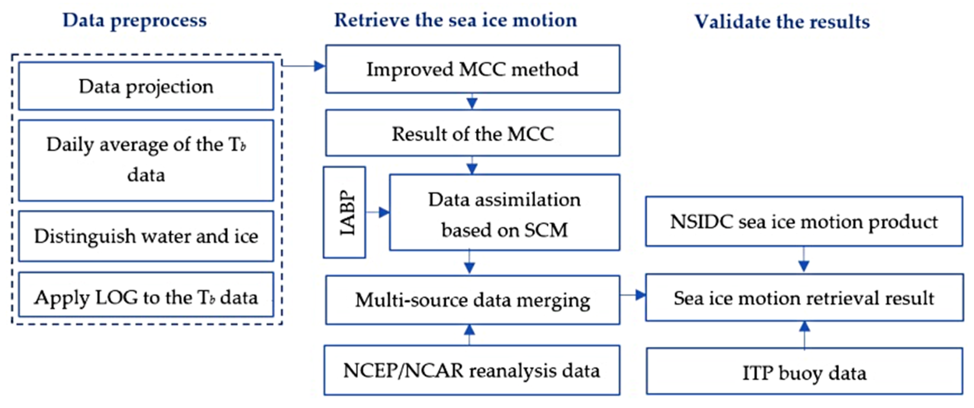
2.2. Data Preprocessing
2.3. SIM Retrieval Method in the Arctic
3. Results
3.1. Retrieval Results of Arctic SIM Based on Modified MCC Method
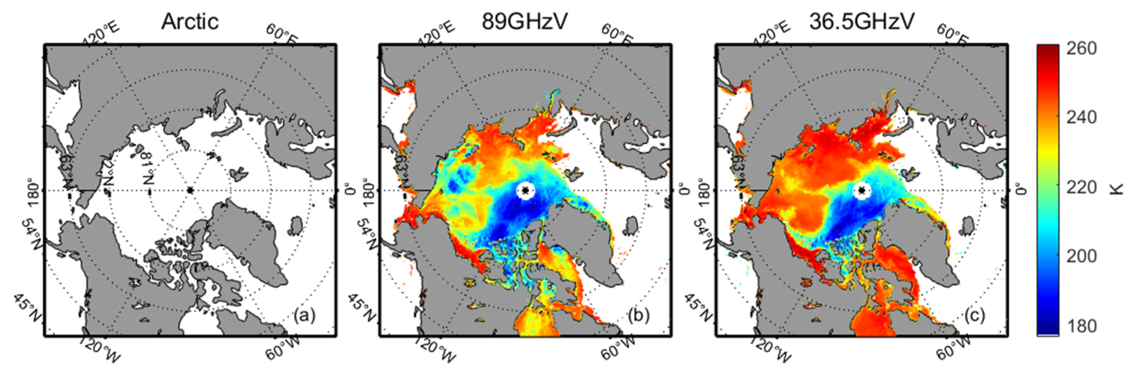
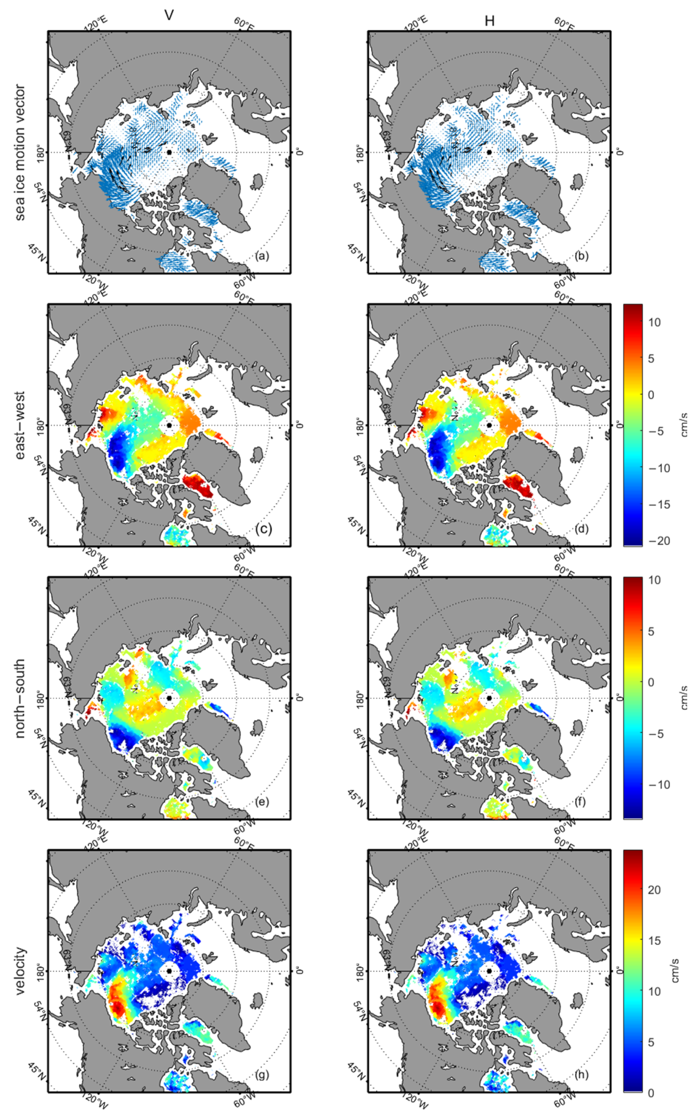
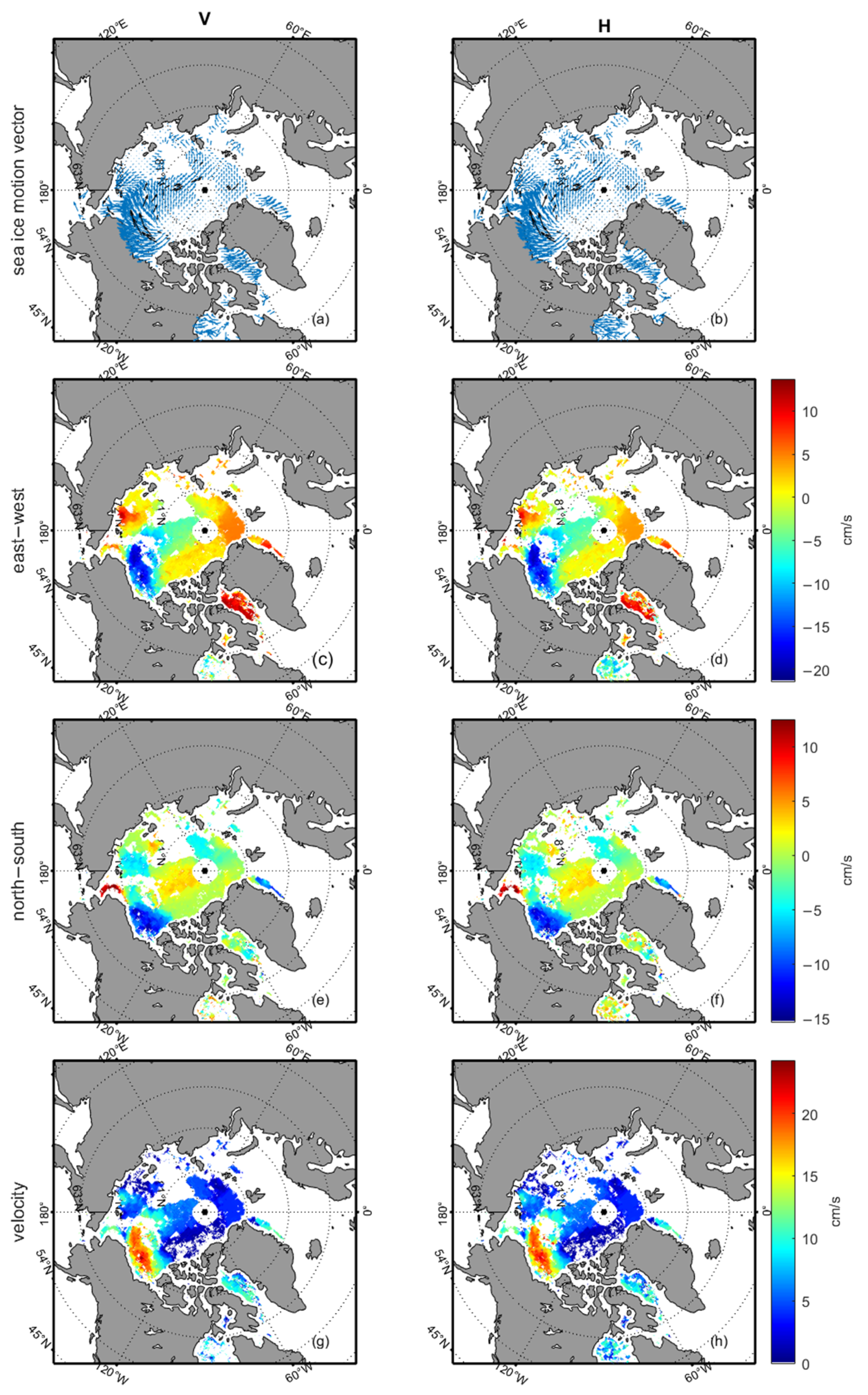
3.1.1. SIM Inversion from Tb Data with Different Polarization
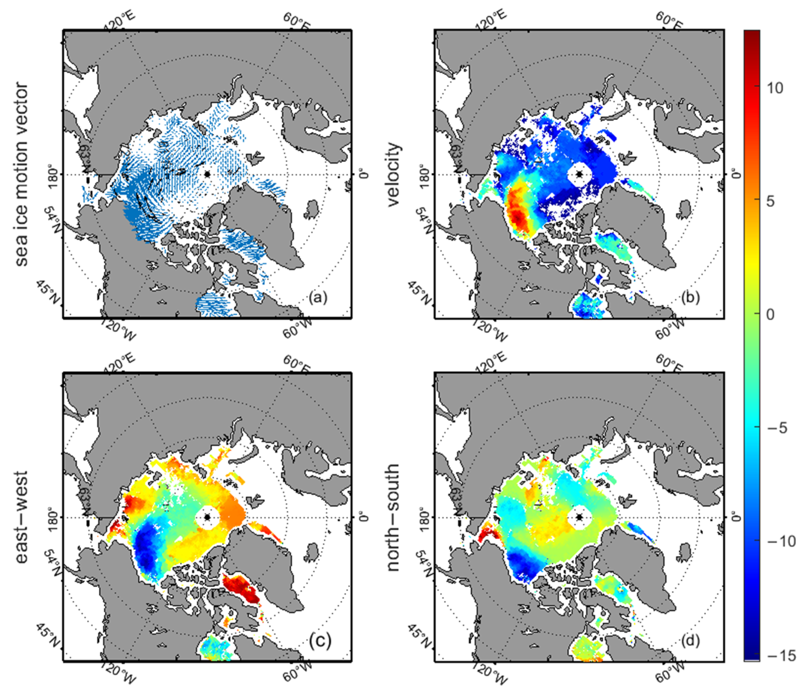
3.1.2. Merging SIM from FY-3D/MWRI Tb Data at Different Frequencies
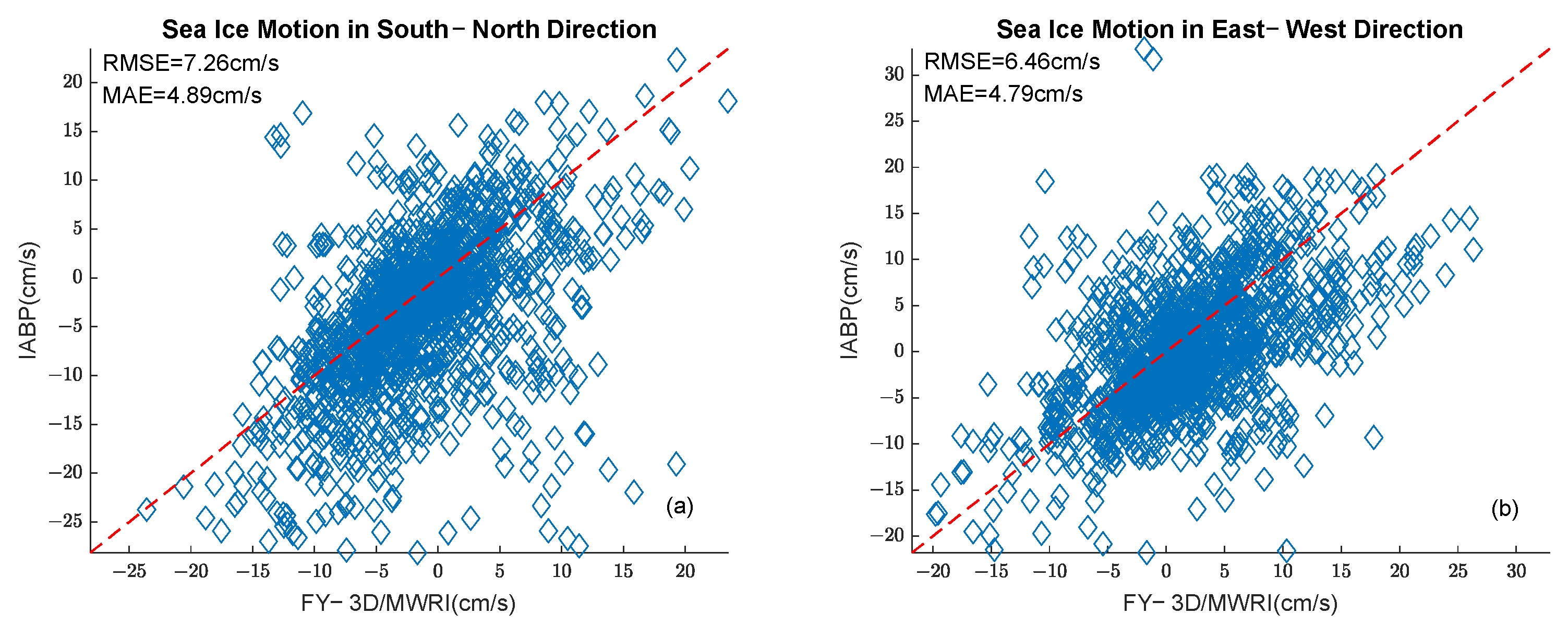
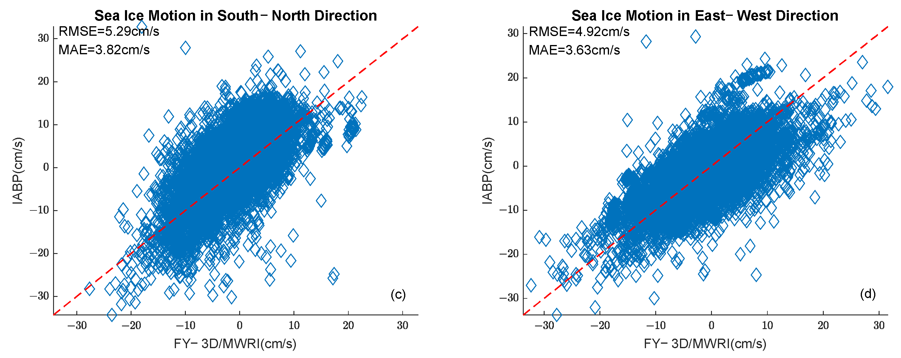
3.2. Multisource Data Merging
4. Discussion
5. Conclusions
Author Contributions
Funding
Data Availability Statement
Acknowledgments
Conflicts of Interest
References
- Holland, M.M.; Bitz, C.M. Polar amplification of climate change in coupled models. Clim. Dyn. 2003, 21, 221–232. [Google Scholar] [CrossRef]
- Comiso, J.C.; Hall, D.K. Climate trends in the Arctic as observed from space. Wiley Interdiscip. Rev.-Clim. Chang. 2014, 5, 389–409. [Google Scholar] [CrossRef]
- Liu, N.; Chen, H.; Ni, K.; Li, L. Retrieval of Thin Ice Thickness from FY-3D/MWRI Brightness Temperature in the Arctic. Master’s Thesis, The Ocean University of China, Qingdao, China, 2022. [Google Scholar]
- Zuo, Z.D. The Characteristics of Arctic Sea Ice Motion and the Effects of Arctic Cyclone on It. Master’s Thesis, Shanghai Ocean University, Shanghai, China, 2016. [Google Scholar]
- Kang, J.C.; Yan, Q.D.; Sun, B.; Meng, G.L.; Kumiko, G. The arctic sea ice, climate and its relation with global climate system. Chin. J. Polar Res. 1999, 4, 301–310. [Google Scholar]
- Gui, D. Characteristics of Sea Ice Motion and Deformation in the Arctic Using Sea Ice Motion Product. Ph.D. Thesis, Wuhan University, Wuhan, China, 2020. [Google Scholar]
- Williams, W.J.; Carmack, E.C.; Shimada, K.; Meling, H.; Aagaard, K.; Macdonald, R.W.; Grant Ingram, R. Joint effects of wind and ice motion in forcing upwelling in Mackenzie Trough. Beaufort Sea. Cont. Shelf Res. 2006, 26, 2352–2366. [Google Scholar] [CrossRef]
- Holland, M.M.; Bitz, C.M.; Eby, M.; Weaver, A.J. The Role of Ice-Ocean Interactions in the Variability of the North Atlantic Thermohaline Circulation. J. Clim. 2001, 14, 656–675. [Google Scholar] [CrossRef]
- Peiji, L. The Arctic Sea Ice and Climate Change. J. Glaciol. Geocryol. 1996, 1, 74–82. [Google Scholar]
- Mauritzen, C.; Häkkinen, S. Influence of sea ice on the thermohaline circulation in the Arctic-North Atlantic Ocean. Geophys. Res. Lett. 1997, 24, 3257–3260. [Google Scholar] [CrossRef]
- Wang, X.; Lei, G.; Li, L. Comparison and validation of sea ice concentration from FY-3B/MWRI and Aqua/AMSR-E observations. Natl. Remote Sens. Bull. 2018, 22, 723–736. [Google Scholar] [CrossRef]
- Li, L.; Chen, H.; Wang, X.; Guan, L. Study on the Retrieval of Sea Ice Concentration from Fy3b/Mwri in the Arctic. In Proceedings of the 2019 IEEE 39th International Geoscience and Remote Sensing Symposium (IGARSS), Yokohama, Japan, 28 July–2 August 2019; pp. 4242–4245. [Google Scholar]
- Li, L.; Chen, H.; Guan, L. Retrieval of snow depth on sea ice in the Arctic using the FengYun-3B microwave radiation imager. J. Ocean. Univ. Chin. 2019, 18, 580–588. [Google Scholar] [CrossRef]
- Ni, K.; Chen, H.; Li, L.; Meng, X. Retrieving the Motion of Beaufort Sea Ice Using Brightness Temperature Data from FY-3D Microwave Radiometer Imager. Sensors 2022, 22, 8298. [Google Scholar] [CrossRef]
- Ninnis, R.M.; Emery, W.J.; Collins, M.J. Automated extraction of pack ice motion from advanced very high resolution radiometer imagery. J. Geophys. Res.-Ocean. 1986, 91, 10725–10734. [Google Scholar] [CrossRef]
- Kwok, R.; Curlander, J.C.; McConnell, R.; Pang, S.S. An ice-motion tracking system at the Alaska SAR facility. IEEE J. Ocean. Eng. 1990, 15, 44–54. [Google Scholar] [CrossRef]
- Martin, T.; Augstein, E. Large-scale drift of Arctic Sea ice retrieved from passive microwave satellite data. J. Geophys. Res. 2000, 105, 8775–8788. [Google Scholar] [CrossRef]
- Lavergne, T.; Eastwood, S.; Teffah, Z.; Schyberg, H.; Breivik, L.A. Sea ice motion from low-resolution satellite sensors: An alternative method and its validation in the Arctic. J. Geophys. Res. Ocean. 2010, 115, C10032. [Google Scholar] [CrossRef]
- Ezraty, R.; Girard-Ardhuin, F.; Croizé-Fillon, D. Sea Ice Drift in the Central Arctic using the 89 GHz Brightness Temperature of the Advanced Microwave Scanning Radiometer—User’s Manual 2.0. French Research Institute for the Exploitation of the Seas (Ifremer). 2007. Available online: ftp://ftp.ifremer.fr/ifremer/cersat/products/gridded/psi-drift/documentation/amsr.pdf (accessed on 26 August 2022).
- Liu, A.K.; Cavalieri, D.J. On sea ice drift from the wavelet analysis of the Defense Meteorological Satellite Program (DMSP) Special Sensor Microwave Imager (SSM/I) data. Int. J. Remote Sens. 1998, 19, 1415–1423. [Google Scholar] [CrossRef]
- Wang, L.; He, Y.; Zhang, B.; Liu, B. Retrieval of Arctic sea ice drift using HY-2 satellite scanning microwave radiometer data. Haiyang Xuebao 2017, 39, 110–120. [Google Scholar]
- Komarov, A.S.; Barber, D.G. Sea Ice Motion Tracking from Sequential Dual-Polarization RADARSAT-2 Images. IEEE Trans. Geosci. Remote Sens. 2014, 52, 121–136. [Google Scholar] [CrossRef]
- Howell, S.E.L.; Brady, M.; Komarov, A.S. Generating large-scale sea ice motion from Sentinel-1 and the RADARSAT Constellation Mission using the Environment and Climate Change Canada automated sea ice tracking system. Cryosphere 2022, 16, 1125–1139. [Google Scholar] [CrossRef]
- Muckenhuber, S.; Sandven, S. Open-source sea ice drift algorithm for Sentinel-1 SAR imagery using a combination of feature tracking and pattern matching. Cryosphere 2017, 11, 1835–1850. [Google Scholar] [CrossRef]
- Li, C.; Li, G.; Chen, Z.; Wang, X.; Cheng, X. Matching Vector Filtering Methods for Sea Ice Motion Detection Using SAR Imagery Feature Tracking. IEEE J. Sel. Top. Appl. Earth Obs. Remote Sens. 2022, 15, 6197–6202. [Google Scholar] [CrossRef]
- Hwang, B. Inter-comparison of satellite sea ice motion with drifting buoy data. Int. J. Remote Sens. 2013, 34, 8741–8763. [Google Scholar] [CrossRef]
- Shi, Q.; Su, J.; Spreen, G.; Yang, Q. An Improved Sea-Ice Velocity Retrieval Algorithm Based on 89 GHz Brightness Temperature Satellite Data in the Fram Strait. Earth Space Sci. 2022, 9, e2021EA002170. [Google Scholar] [CrossRef]
- Wang, X.; Chen, R.; Li, C.; Chen, Z.; Hui, F.; Cheng, X. An Intercomparison of Satellite Derived Arctic Sea Ice Motion Products. Remote Sens. 2022, 14, 1261. [Google Scholar] [CrossRef]
- Kalnay, E.; Kanamitsu, M.; Kistler, R.; Collins, W.; Deaven, D.; Gandin, L.; Iredell, M.; Saha, S.; White, G.; Woollen, J.; et al. The NCEP/NCAR 40-Year Reanalysis Project. Bull. Amer. Meteorol. Soc. 1996, 77, 437–472. [Google Scholar] [CrossRef]
- Tschudi, M.; Meier, W.N.; Stewart, J.S.; Fowler, C.; Maslanik, J. Polar Pathfinder Daily 25 km EASE-Grid Sea Ice Motion Vectors; Version 4. [The Arctic Region]; NASA National Snow and Ice Data Center Distributed Active Archive Center: Boulder, CO, USA, 2019. [CrossRef]
- Tschudi, M.; Meier, W.; Stewart, J. An enhancement to sea ice motion and age products at the National Snow and Ice Data Center (NSIDC). Cryosphere 2020, 14, 1519–1536. [Google Scholar] [CrossRef]
- Kalnay, E. Atmospheric Modeling Data Assimilation and Predictability, 1st ed.; China Meteorological Press: Beijing, China, 2005; pp. 115–119. [Google Scholar]
- Bergthorsson, P.; Döös, B.R.; Fryklund, S.; Haug, O.; Lindquist, R. Routine Forecasting with the Barotropic Model. Tellus 1955, 7, 272–274. [Google Scholar] [CrossRef]
- Cressman, G.P. An Operational Objective Analysis System. Mon. Weather. Rev. 1959, 87, 367–374. [Google Scholar] [CrossRef]


| 36.5 GHz | 89 GHz | |||
|---|---|---|---|---|
| H | V | H | V | |
| Winter | 9764 | 10,607 | 8472 | 9098 |
| Summer | 617 | 1032 | 468 | 590 |
| Total number | 10,381 | 11,639 | 8940 | 9688 |
| H | V | ||||
|---|---|---|---|---|---|
| East–West cm/s) | North–South cm/s) | East–West cm/s) | North–South cm/s) | ||
| Winter | January | 2.42/3.33 | 2.58/3.83 | 2.43/3.36 | 2.62/3.83 |
| February | 3.95/4.85 | 3.39/4.33 | 3.88/4.70 | 3.30/4.29 | |
| March | 2.35/3.43 | 2.52/3.63 | 2.34/3.39 | 2.52/3.72 | |
| April | 3.22/4.39 | 3.28/4.41 | 3.22/4.46 | 3.13/4.24 | |
| May | 3.51/4.91 | 4.56/6.47 | 3.49/4.67 | 4.09/5.74 | |
| Summer | June | 4.73/6.40 | 5.63/8.36 | 4.74/6.69 | 4.64/7.24 |
| July | 6.27/8.78 | 5.83/8.77 | 5.58/7.72 | 7.05/10.72 | |
| August | 7.3/10.05 | 7.38/11.1 | 6.72/8.89 | 7.53/10.23 | |
| September | 5.81/7.54 | 5.00/7.55 | 5.08/6.91 | 4.60/6.87 | |
| Winter | October | 3.51/4.76 | 5.17/6.57 | 3.43/4.57 | 5.13/6.55 |
| November | 4.92/6.25 | 5.21/6.68 | 4.84/6.17 | 5.08/6.44 | |
| December | 4.33/5.77 | 4.57/6.01 | 4.28/5.73 | 4.55/5.91 | |
| January–December | 3.70/5.07 | 4.06/5.62 | 3.65/4.98 | 3.97/5.50 | |
| H | V | ||||
|---|---|---|---|---|---|
| East–West cm/s) | North–South cm/s) | East–West cm/s) | North–South cm/s) | ||
| Winter | January | 2.50/3.51 | 2.50/3.66 | 2.50/3.50 | 2.56/3.75 |
| February | 4.12/5.09 | 3.24/4.22 | 4.11/5.04 | 3.28/4.33 | |
| March | 2.41/3.51 | 2.60/4.05 | 2.36/3.49 | 2.45/3.51 | |
| April | 3.10/4.27 | 2.88/4.05 | 3.12/4.25 | 3.00/4.23 | |
| May | 2.95/3.99 | 3.41/4.78 | 3.16/4.27 | 3.56/4.99 | |
| Summer | June | 3.88/5.14 | 4.28/5.70 | 4.77/6.65 | 4.85/7.44 |
| July | 3.82/5.33 | 3.94/6.05 | 4.69/6.47 | 5.01/7.02 | |
| August | 5.19/6.65 | 5.74/8.37 | 5.83/7.94 | 5.46/7.88 | |
| September | 4.61/6.37 | 4.28/6.34 | 4.40/5.82 | 4.15/6.03 | |
| Winter | October | 3.32/4.46 | 4.83/6.24 | 3.46/4.58 | 4.73/6.10 |
| November | 4.93/6.31 | 4.81/6.16 | 4.85/6.12 | 4.83/6.20 | |
| December | 4.01/5.39 | 4.41/5.89 | 4.34/5.89 | 4.47/5.98 | |
| January–December | 3.59/4.89 | 3.73/5.15 | 3.69/5.01 | 3.81/5.28 | |
| East–West (cm/s) | North–South (cm/s) | ||
|---|---|---|---|
| Winter | January | 2.56/3.60 | 2.62/3.84 |
| February | 4.12/5.10 | 3.27/4.36 | |
| March | 2.41/3.55 | 2.56/3.97 | |
| April | 3.26/4.47 | 3.26/4.34 | |
| May | 3.28/4.42 | 3.74/5.28 | |
| Summer | June | 4.70/6.31 | 5.18/7.84 |
| July | 4.64/6.53 | 4.96/7.39 | |
| August | 5.82/7.84 | 6.15/8.90 | |
| September | 4.55/5.97 | 4.29/6.20 | |
| Winter | October | 3.53/4.74 | 4.72/6.13 |
| November | 4.79/6.06 | 4.92/6.36 | |
| December | 4.39/5.92 | 4.61/6.15 | |
| 2019 | January–December | 3.76/5.11 | 3.94/5.54 |
| Winter | Summer | Total Number | |
|---|---|---|---|
| Number of matching points | 11,595 | 1454 | 13,049 |
| East–West (AE/RMSE(cm/s)) | North–South (AE/RMSE(cm/s)) | Sea Ice Velocity (AE/RMSE(cm/s)) | |
|---|---|---|---|
| January | 0.26/0.88 | 0.24/0.76 | −0.94/0.89 |
| February | 1.47/0.99 | −0.13/0.85 | −0.88/0.99 |
| March | 0.66/0.95 | 0.18/0.89 | −0.91/0.95 |
| April | −0.63/0.79 | 0.26/0.83 | −0.33/0.79 |
| May | −1.04/0.68 | 0.39/0.72 | 0.32/0.69 |
| June | −0.29/0.58 | −0.30/0.56 | 0.35/0.58 |
| July | −0.38/0.49 | −0.08/0.50 | 0.51/0.49 |
| August | 0.19/0.40 | 0.27/0.38 | 0.49/0.40 |
| September | −0.19/0.41 | 0.75/0.45 | 0.36/0.41 |
| October | −0.38/0.81 | −0.90/0.90 | 0.50/0.81 |
| November | 0.044/0.76 | −0.02/0.66 | 0.02/0.76 |
| December | −0.35/0.69 | 0.33/0.70 | −0.36/0.69 |
| winter | 0.29/0.83 | 0.27/0.79 | −0.76/0.77 |
| summer | −0.20/0.47 | −0.03/0.45 | 0.36/0.49 |
| FY-3D/MWRI | NSIDC | |||
|---|---|---|---|---|
| East–West (cm/s) | North–South (cm/s) | East–West (cm/s) | North–South (cm/s) | |
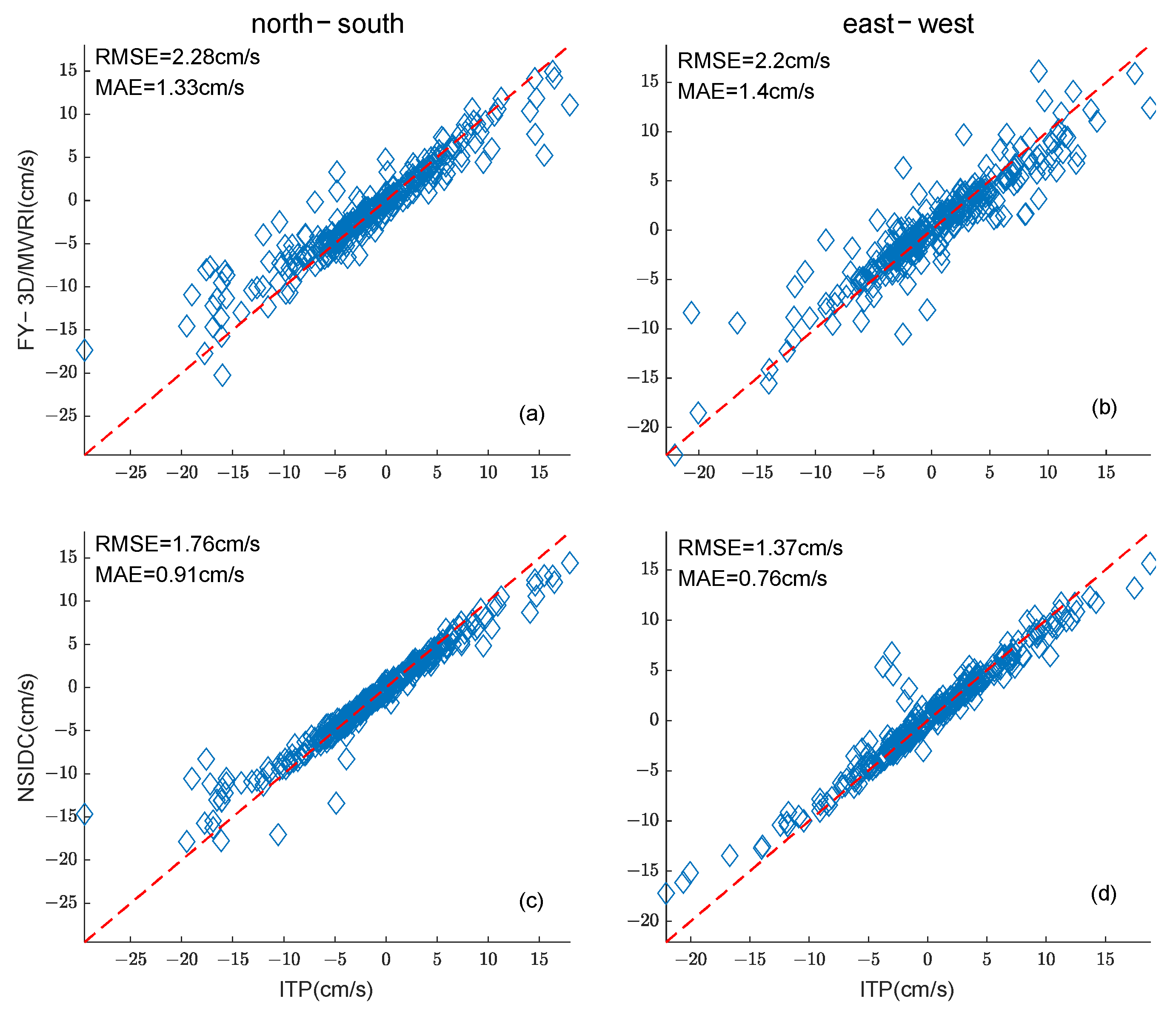
| Summer | 1.40/2.20 | 1.33/2.28 | 0.76/1.37 | 0.91/1.76 |
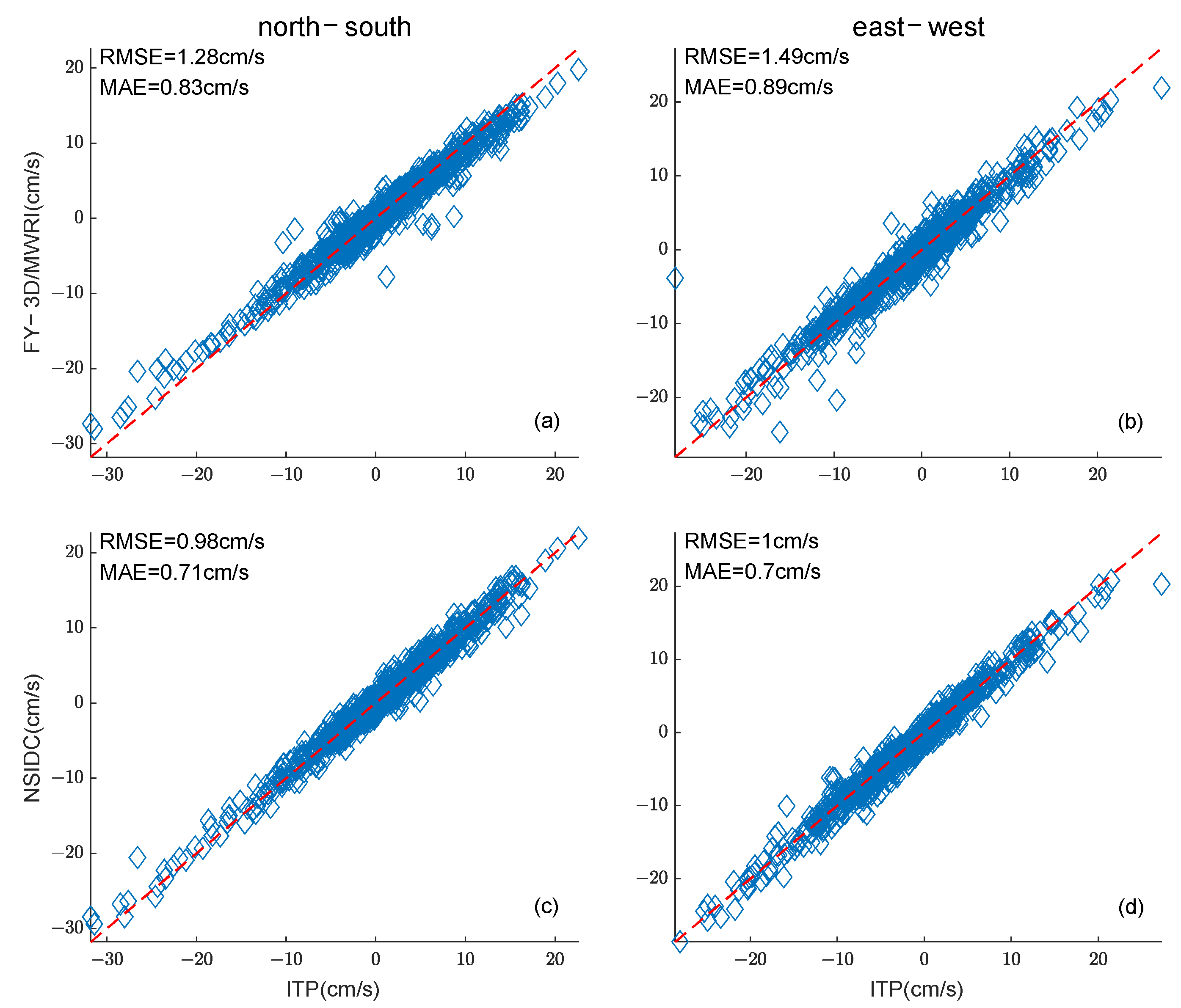
| Winter | 0.89/1.49 | 0.83/1.28 | 0.70/1.00 | 0.71/0.98 |
| 2019 | 1.01/1.68 | 0.95/1.56 | 0.71/1.09 | 0.76/1.20 |
| FY-3D/MWRI | NSIDC | |||
|---|---|---|---|---|
| Time | East–West APE (%) | North–South APE (%) | East–West APE (%) | North–South APE (%) |
| Summer | −12.67 | −13.94 | −5.20 | −7.98 |
| Winter | −4.64 | −6.13 | −3.15 | −5.19 |
| 2019 | −6.54 | −7.92 | −3.62 | −5.81 |
Disclaimer/Publisher’s Note: The statements, opinions and data contained in all publications are solely those of the individual author(s) and contributor(s) and not of MDPI and/or the editor(s). MDPI and/or the editor(s) disclaim responsibility for any injury to people or property resulting from any ideas, methods, instructions or products referred to in the content. |
© 2023 by the authors. Licensee MDPI, Basel, Switzerland. This article is an open access article distributed under the terms and conditions of the Creative Commons Attribution (CC BY) license (https://creativecommons.org/licenses/by/4.0/).
Share and Cite
Chen, H.; Ni, K.; Liu, J.; Li, L. Retrieval of Arctic Sea Ice Motion from FY-3D/MWRI Brightness Temperature Data. Remote Sens. 2023, 15, 4191. https://doi.org/10.3390/rs15174191
Chen H, Ni K, Liu J, Li L. Retrieval of Arctic Sea Ice Motion from FY-3D/MWRI Brightness Temperature Data. Remote Sensing. 2023; 15(17):4191. https://doi.org/10.3390/rs15174191
Chicago/Turabian StyleChen, Haihua, Kun Ni, Jun Liu, and Lele Li. 2023. "Retrieval of Arctic Sea Ice Motion from FY-3D/MWRI Brightness Temperature Data" Remote Sensing 15, no. 17: 4191. https://doi.org/10.3390/rs15174191