
Spatiotemporal Evaluation of the Flood Potential Index and Its Driving Factors across the Volga River Basin Based on Combined Satellite Gravity Observations

 , ,
, ,
Abstract
:1. Introduction
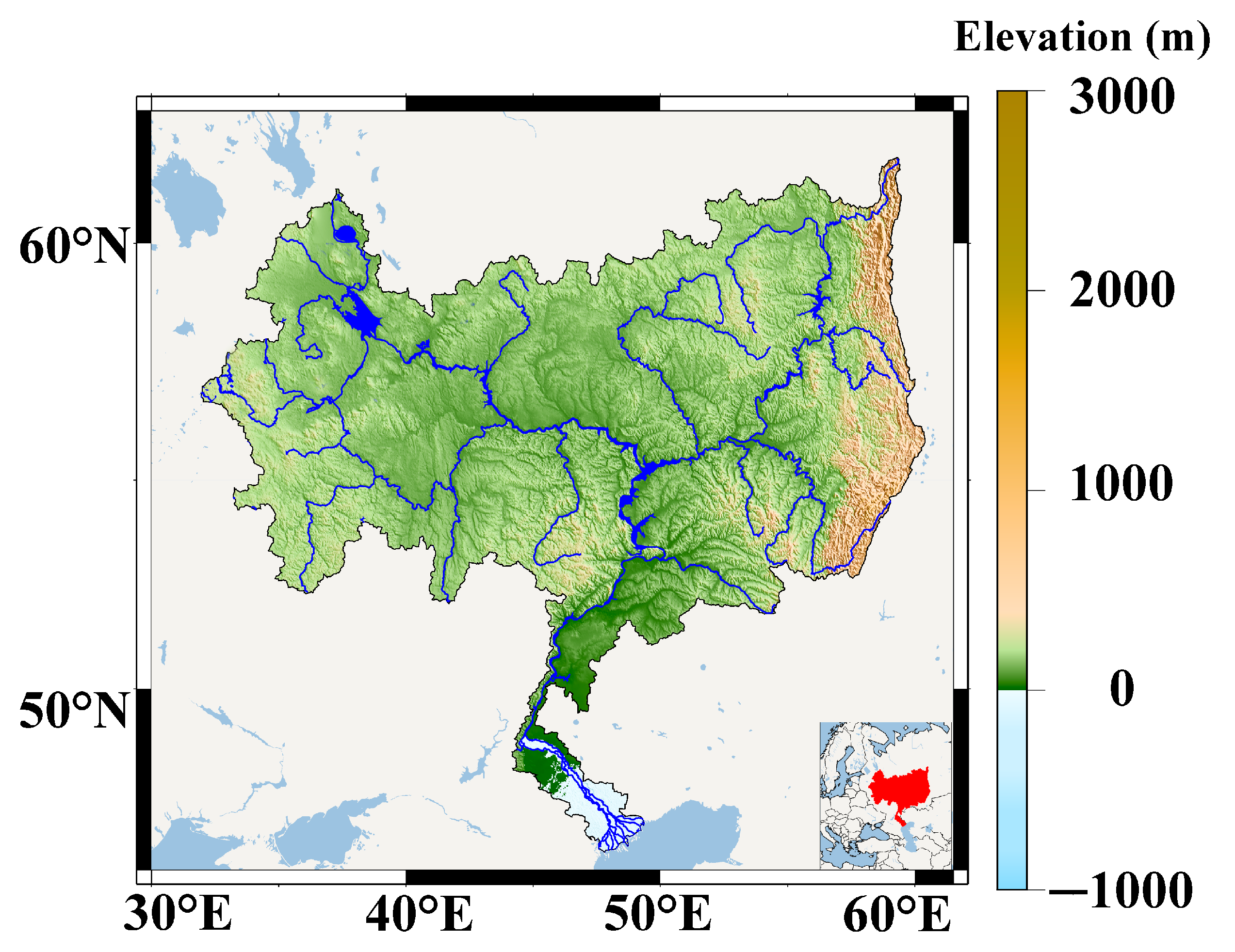
2. Study Areas
3. Data and Methods
3.1. Data
3.1.1. GRACE/GRACE-FO Data
3.1.2. Swarm Solution
3.1.3. PPT Data
3.1.4. ET Data
3.1.5. Other Hydrometeorological Data
3.2. Method
3.2.1. Data Fusion
3.2.2. FPI Calculation
3.2.3. Time Series Analysis
3.2.4. Partial Least Square Regression Model (PLSR)
3.2.5. Correlation Coefficient and Delay Months
4. Results
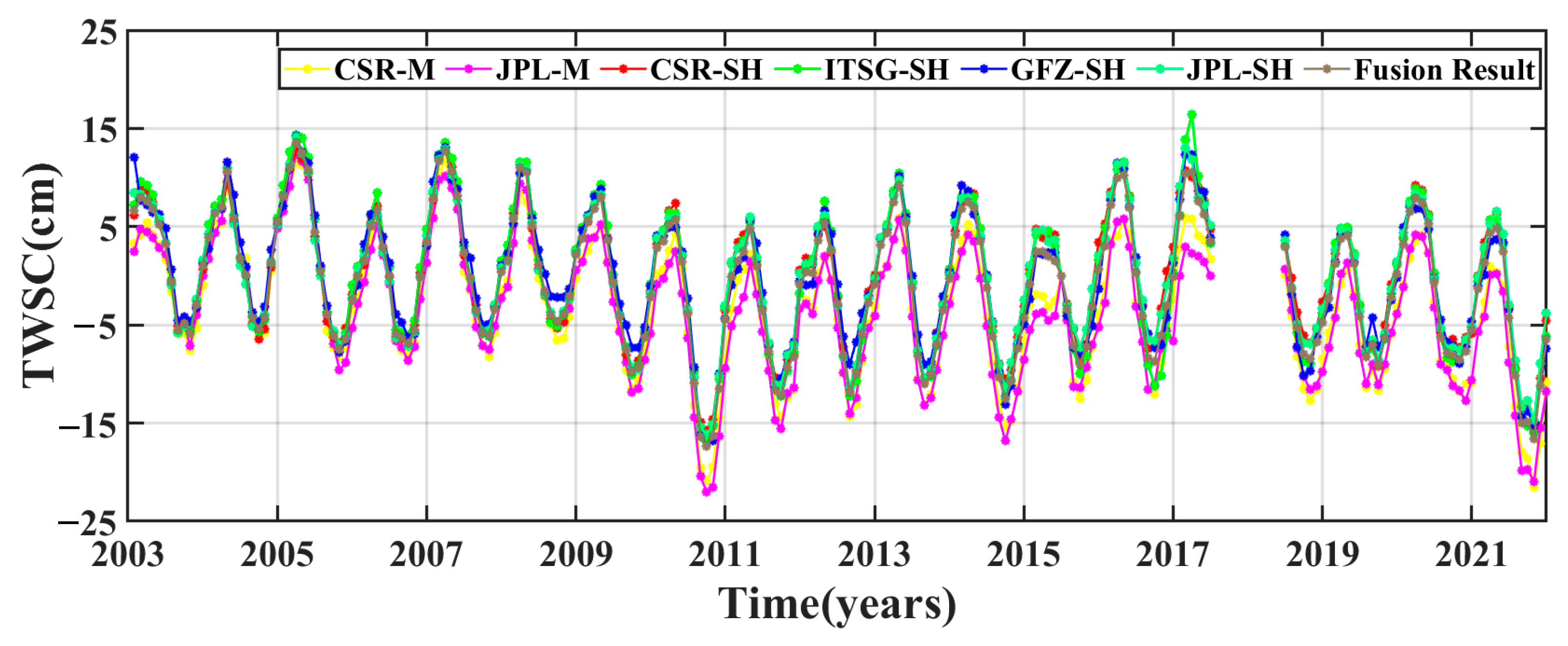
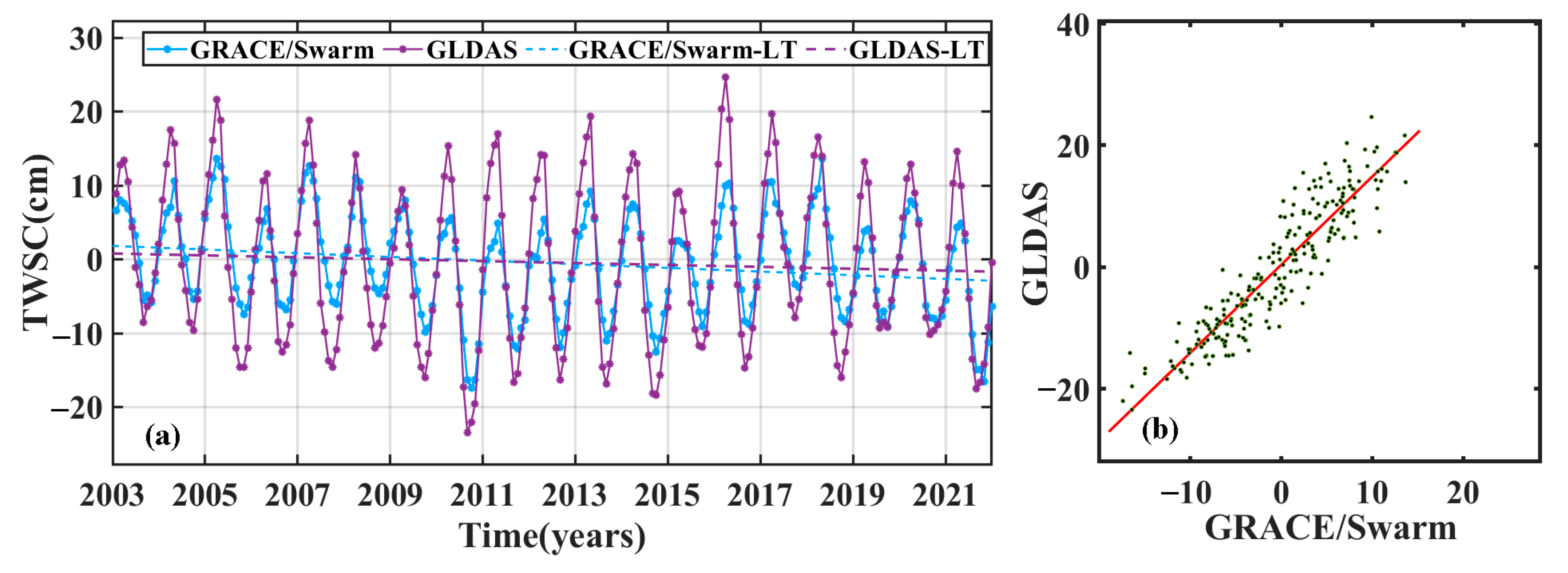
4.1. Construction of Combined TWSC Observation
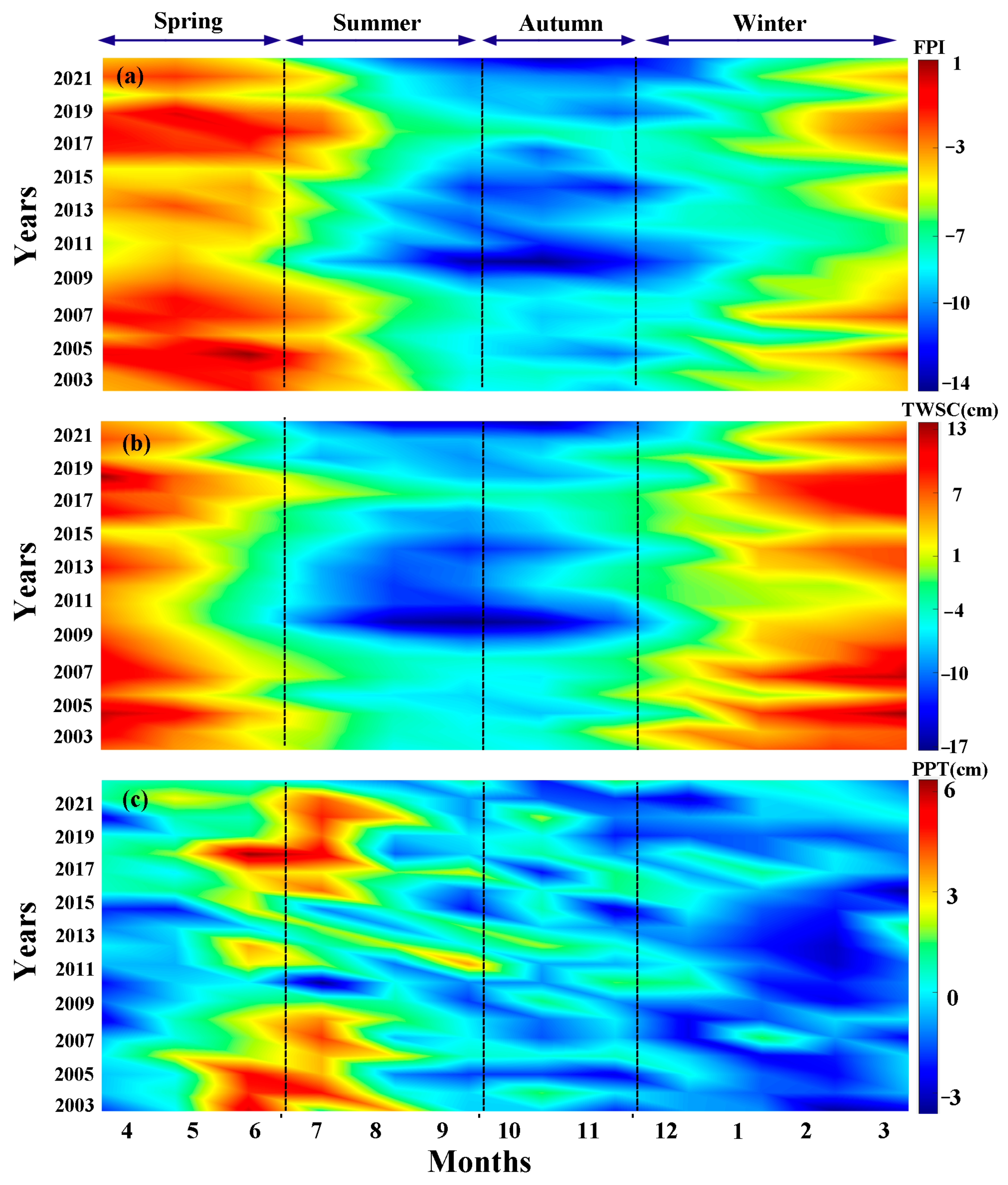
4.2. Spatial and Temporal Characteristics of the FPI
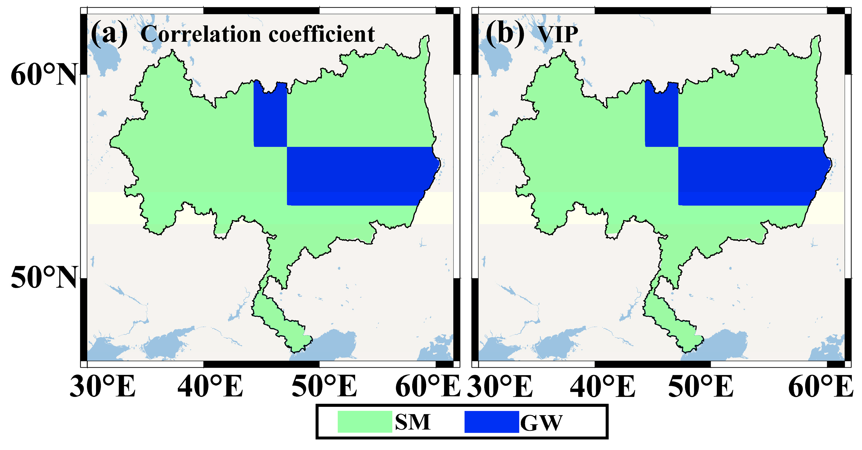
4.3. Influencing Factors on the FPI
5. Discussion
5.1. Path of Flood Formation
5.2. Uncertainty of the FPI
5.3. Future Direction
6. Conclusions
- (1)
- The uncertainty of the fused TWSC results (0.76 cm) is much lower than the uncertainty of any single solution (the average is 2.14 cm), and the Swarm TWSC results have a good consistency with the GRACE results (correlation coefficient is 0.82) in the VRB. The TWSC time series estimated by combining the fused result and Swarm solution has the same performance as the ones from the GLDAS model.
- (2)
- On the seasonal scale, spring and autumn are the seasons with the greatest and smallest FPI, respectively. With regards to spatial distribution, the FPI is rising in the north and falling in the south, so the north is more prone to floods than the south. In the study period, there were two extreme floods detected by the FPI in the VRB.
- (3)
- Since SWE is an important source of recharge for water resources in the VRB, it has a strong correlation with the FPI. SWE is vulnerable to ST. Snow melts faster when the ST rises. And more water in runoff and SM comes from SWE than PPT. Therefore, the abnormal changes in SWE have a very important impact on the floods in the VRB, and the effect of SWE on the floods is greater than that of PPT.
Author Contributions
Funding
Institutional Review Board Statement
Informed Consent Statement
Data Availability Statement
Acknowledgments
Conflicts of Interest
References
- Hall, J.; Arherimer, B.; Borga, M.; Brázdil, R.; Claps, P.; Kiss, A.; Kjeldsen, T.; Kriaučiūniene, J.; Kundzewica, Z.; Lang, M.; et al. Understanding flood regime changes in Europe: A state-of-the-art assessment. Hydol. Earth Syst. Sci. 2014, 18, 2735–2772. [Google Scholar]
- Cui, L.; He, M.; Zou, Z.; Yao, C.; Wang, S.; An, J.; Wang, X. The influence of climate change on droughts and floods in the Yangtze River basin from 2003 to 2020. Sensors 2022, 22, 8178. [Google Scholar] [PubMed]
- Fang, J.; Kong, F.; Fang, J.; Zhao, L. Observed changes in hydrological extreme and flood disaster in Yangtze River Basin: Spatial-temporal variability and climate change impacts. Nat. Hazards 2018, 93, 89–107. [Google Scholar]
- Zhao, Q.; Ding, Y.; Wang, J.; Gao, H.; Zhang, S.; Zhao, C.; Xu, J.; Han, H.; Shangguan, D. Projecting climate change impacts on hydrological processes on the Tibetan Plateau with model calibration against the glacier inventory data and observed streamflow. J. Hydrol. 2019, 573, 60–81. [Google Scholar]
- IPCC. Climate Change 2021: The Physical Science Basis. Contribution of Working Group I to the Sixth Assessment Report of the Intergovernmental Panel on Climate Change; Cambridge University Press: Cambridge, UK, 2021. [Google Scholar]
- Hirabayashi, Y.; Mahendran, R.; Koirala, S.; Konoshima, L.; Yamazaki, D.; Watanabe, S.; Kim, H.; Kanae, S. Global flood risk under climate change. Nat. Clim. Chang. 2013, 3, 816–821. [Google Scholar]
- Arnell, N.; Gosling, S. The impacts of climate change on river flood risk at the global scale. Clim. Chang. 2016, 134, 387–401. [Google Scholar]
- Tabari, H. Climate change impact on flood and extreme precipitation increases with water availability. Sci. Rep. 2020, 10, 13768. [Google Scholar]
- Khalequzzaman, M. Recent Floods in Bangladesh-possible causes and solutions. Nat. Hazards 1994, 9, 65–80. [Google Scholar]
- Persoons, E.; Vanclooster, M.; Desmed, A. Flood hazard causes and flood protection recommendations for Belgian river basins. Water Int. 2002, 27, 202–207. [Google Scholar]
- Marengo, J.; Espinoza, J. Extreme seasonal drought and floods in Amazonia: Causes, trends and Impacts. Int. J. Climatol. 2016, 36, 1033–1050. [Google Scholar]
- Dahri, N.; Abida, H. Causes and impacts of flash floods: Case of Gabes City, Southern Tunisia. Arab. J. Geosci. 2020, 13, 176. [Google Scholar]
- Hughes, A.; Vounaki, T.; Peach, D.; Ireson, A.; Jackson, C.; Butler, A.; Bloomfield, J.; Finch, J.; Wheater, H. Flood risk from groundwater: Examples from a Chalk catchment in southern England. J. Flood Risk Manag. 2011, 4, 143–155. [Google Scholar]
- Att-ur, R.; Amir, N. Analysis of flood causes and associated socio-economic damage in the Hindukush region. Nat. Hazards 2011, 59, 1239–1260. [Google Scholar] [CrossRef]
- Zhong, M.; Zeng, T.; Jiang, T.; Wu, H.; Chen, X.; Hong, Y. A copula-based multivariate probability analysis for flash flood risk under the compound effect of soil moisture and rainfall. Water Res. Manag. 2021, 35, 83–98. [Google Scholar] [CrossRef]
- Hagen, E.; Lu, X. Let us create flood hazard maps for developing countries. Nat. Hazards 2011, 58, 841–843. [Google Scholar] [CrossRef]
- Hossain, F.; Lettenmaier, D. Flood prediction in the future: Recognizing hydrologic issues in anticipation of the Global Precipitation Measurement mission. Water Resour. Res. 2006, 42, W11301. [Google Scholar]
- Clark, M.; Fan, Y.; Lawrence, D.; Adam, J.; Bolster, D.; Gochis, D.; Hooper, R.; Kumar, M.; Leung, L.; Mackay, D.; et al. Improving the representation of hydrologic processes in Earth System Models. Water Resour. Res. 2015, 51, 5929–5956. [Google Scholar]
- Wang, Y.; Chen, A.; Fu, G.; Djordjevic, S.; Zhang, C.; Savic, D. An integrated framework for high-resolution urban flood modelling considering multiple information sources and urban features. Environ. Model. Softw. 2018, 107, 85–95. [Google Scholar]
- Girotto, M.; Rodell, M. Chapter Two-Terrestrial water storage. In Extreme Hydro-Climatic Events and Multivariate Hazards in a Changing Environment; Maggioni, V., Massari, C., Eds.; Elsevier: Amsterdam, The Netherlands, 2019; pp. 41–46. [Google Scholar]
- Mohamed, A.; Faye, C.; Othman, A.; Abdelrady, A. Hydro-geophysical evaluation of the regional variability of Senegal’s terrestrial water storage using time-variable gravity data. Remote Sens. 2022, 14, 4059. [Google Scholar] [CrossRef]
- Chen, J.; Wilson, C.; Tapley, B. The 2009 exceptional Amazon flood and inter annual terrestrial water storage change observed by GRACE. Water Resour. Res. 2010, 46, W12526. [Google Scholar]
- Li, B.; Rodell, M.; Zaitchik, B.; Reichle, R.; Koster, R.; Dam, T. Assilation of GRACE terrestrial water storage into a land surface model: Evaluation and potential value for drought monitoring in western and central Europe. J. Hydrol. 2012, 446–447, 103–105. [Google Scholar]
- Wang, L.; Peng, Z.; Ma, X.; Zheng, Y.; Chen, C. Multiscale gravity measurements to characterize 2020 flodd events and their spatio-temporal evolution in Yangtze River of China. J. Hydrol. 2021, 603, 127176. [Google Scholar]
- Yan, X.; Zhang, B.; Yao, Y.; Yin, J.; Wang, H.; Ran, Q. Jointly using the GLDAS2.2 model and GRACE to study the severe Yangtze flooding of 2020. J. Hydrol. 2022, 610, 127927. [Google Scholar]
- Nigatu, Z.; Fan, D.; You, W.; Melesse, A. Hydroclimatic extremes evaluation using GRACE/GRACE-FO and multidecadal climatic variables over the Nile River basin. Remote Sens. 2021, 13, 651. [Google Scholar]
- Idowu, D.; Zhou, W. Performance evaluation of a potential component of an early flood warning system—A case study of the 2012 flood, lower Niger River basin, Nigeria. Remote Sens. 2019, 11, 1970. [Google Scholar] [CrossRef]
- Chen, X.; Jiang, J.; Li, H. Drought and flood monitoring of the Liao River basin in northeast China using extended GRACE data. Remote Sens. 2018, 10, 1168. [Google Scholar]
- Cui, L.; Song, Z.; Luo, Z.; Zhong, B.; Wang, X.; Zou, Z. Comparison of terrestrial water storage changes derived from GRACE/GRACE-FO and Swarm: A case study in the Amazon River Basin. Water 2020, 12, 3128. [Google Scholar]
- Da Encarnação, T.; Visser, P.; Arnold, D.; Bezdek, A.; Doornbos, E.; Ellmer, M.; Guo, J.; van den IJssel, J.; Iorfida, E.; Jäggi, A.; et al. Description of the multi-approach gravity field models from Swarm GPS data. Earth Syst. Sci. Data 2020, 12, 1385–1417. [Google Scholar]
- Cui, L.; Yin, M.; Huang, Z.; Yao, C.; Wang, X.; Lin, X. The drought events over the Amazon River basin from 2003 to 2020 detected by GRACE/GRACE-FO and Swarm satellites. Remote Sens. 2022, 14, 2887. [Google Scholar]
- Zhang, C.; Shum, C.; Bezdĕk, A.; Bevis, M.; Da Encarnação, T.; Tapley, B. Rapid mass loss in West Antarctica revealed by Swarm gravimetry in the absence of GRACE. Geophys. Res. Letts 2021, 48, e2021GL095141. [Google Scholar]
- Reager, J.; Famigietti, J. Global terrestrial water storage capacity and flood potential using GRACE. Geophys. Res. Lett. 2009, 36, L23402. [Google Scholar]
- Molodtsova, T.; Molodtsov, S.; Kirilenko, A.; Zhang, X.; Vanlooy, J. Evaluating flood potential with GRACE in the United States. Nat. Hazards Earth Syst. Sci. 2016, 16, 1011–1018. [Google Scholar]
- Sun, Z.; Zhu, X.; Pan, Y.; Zhang, J. Assessing terrestrial water storage and flood potential using GRACE data in the Yangzte River basin, China. Remote Sens. 2017, 9, 1011. [Google Scholar]
- Idowu, D.; Zhou, W. Spatiotemporal evaluation of flood potential indices for watershed flood prediction in the Mississippi River basin, USA. Environ. Eng. Geosci. 2021, 27, 319–330. [Google Scholar]
- Gupta, D.; Dhanya, C. The potential of GRACE in assessing the flood potential of Peninsular Indian River basin. Int. J. Remote Sens. 2020, 41, 9009–9038. [Google Scholar] [CrossRef]
- Abelen, S.; Seitz, F.; Abarca-del-Rio, R.; Huentner, A. Droughts and floods in the La Plata basin in soil moisture data and GRACE. Remote Sens. 2015, 7, 7324–7349. [Google Scholar]
- Xiong, J.; Yin, J.; Guo, S.; Gu, L.; Xiong, F.; Li, N. Integrated flood potential index for flood monitoring in the GRACE era. J. Hydrol. 2021, 603, 127115. [Google Scholar]
- Kalugin, A. Hydrological and meteorological variability in the Volga River basin under global warming by 1.5 and 2 degrees. Climate 2022, 10, 107. [Google Scholar]
- Volga River. Available online: http://xxfb.mwr.cn/slbk/zh/zyhl/202004/t20200409_1466531.html (accessed on 9 August 2023).
- Buber, A.; Bolgov, M.; Buber, V. Statistical and water management assessment of the impact of climate change in the reservoir basin of the Volga-Kama cascade on the environment safety of the lower Volga ecosystem. Appl. Sci. 2023, 13, 4768. [Google Scholar] [CrossRef]
- Georgievskii, V.; Grek, E.A.; Grek, E.N.; Lobanova, A.; Molchanova, T. Spatiotemporal changes in extreme runoff characteristics for the Volga basin rivers. Russ. Meteorol. Hydrol. 2018, 43, 633–638. [Google Scholar]
- Wahr, J.; Molenaar, M.; Bryan, F. Time variability of the Earth’s gravity field: Hydrological and oceanic effects and their possible using GRACE. J. Geophys. Res. Soild Earth 1998, 103, 30205–30229. [Google Scholar]
- Cui, L.; Zhang, C.; Yao, C.; Luo, Z.; Wang, X.; Li, Q. Analysis of the influencing factors of drought events based on GRACE data under different climatic conditions: A case study in Mainland China. Water 2021, 13, 2575. [Google Scholar]
- Jean, Y.; Meyer, U.; Jäggi, A. Combination of GRACE monthly gravity field solutions from different processing strategies. J. Geod. 2018, 92, 1313–1328. [Google Scholar]
- National Weather Information Center. Global Atmospheric/Land Surface Reanalysis Products of China Meteorological Administration, 1st ed.; National Weather Information Center: Beijing, China, 2011; pp. 43–49. [Google Scholar]
- Miralles, D.G.; Holmes, T.R.H.; de Jeu, R.A.M.; Gash, H.; Meesters, A.G.C.A.; Dolman, A.J. Global land surface evaporation estimated from satellite-based observations. Hydrol. Earth Syst. Sci. 2011, 15, 453–469. [Google Scholar] [CrossRef]
- Martens, B.D.G.; Miralles, H.; Lievens, H.; van der Schalie, R.; de Jeu, R.A.M.; Férnandez-Prieto, D.; Beck, H.E.; Dorigo, W.A.; Verhoest, N.E.C. GLEAM v3: Satellite-based land evaporation and root-zone soil moisture. Geosci. Model Dev. 2017, 10, 1903–1925. [Google Scholar]
- Rodell, M.; Houser, P.; Jambor, U.E.A.; Gottschalck, J.; Mitchell, K.; Meng, C.; Arsenault, K.; Cosgrove, B.; Radakovich, J.; Bosilovich, M. The global land data assimilation system. Bull. Am. Meteorol. Soc. 2004, 85, 381–394. [Google Scholar] [CrossRef]
- Long, D.; Pan, Y.; Zhou, J.; Chen, Y.; Hou, X.; Hong, Y.; Scanlon, B.; Longuevergne, L. Global analysis of spatiotemporal variability in merged total water storage changes using multiple GRACE products and global hydrological models. Remote Sens. Environ. 2017, 192, 198–216. [Google Scholar]
- Cui, L.; Zhu, C.; Wu, Y.; Yao, C.; Wang, X.; An, J.; Wei, P. Natural- and human-induced influences on terrestrial water storage change in Sichuan, Southwest China from 2003 to 2020. Remote Sens. 2022, 14, 1369. [Google Scholar]
- Bai, H.; Ming, Z.; Zhong, Y.; Zhong, M.; Kong, D.; Ji, B. Evaluation of evapotranspiration for exorheic basins in China using an improved estimate of terrestrial water storage change. J. Hydrol. 2022, 610, 127885. [Google Scholar]
- Cui, L.; Luo, C.; Yao, C.; Zou, Z.; Wu, G.; Li, Q.; Wang, X. The influence of climate change on forest fires in Yunnan province, Southwest China detected by GRACE satellites. Remote Sens. 2022, 14, 712. [Google Scholar]
- Yan, B.; Fang, N.; Zhang, P.C.; Shi, Z. Impacts of land use change on watershed streamflow and sediment yield: An assessment using hydrologic modelling and partial least squares regression. J. Hydrol. 2013, 484, 26–37. [Google Scholar]
- Woldesenbet, T.A.; Elagib, N.A.; Ribbe, L.; Heinrich, J. Hydrological responses to land use/cover changes in the source region of the Upper Blue Nile Basin, Ethiopia. Sci. Total Environ. 2017, 575, 724–741. [Google Scholar] [PubMed]
- Cui, L.; Chen, X.; An, J.; Yao, C.; Su, Y.; Zhu, C.; Li, Y. Spatiotemporal Variation Characteristics of Droughts and Its Connection to Climate Variability and Human Activities in the Pearl River Basin, South China. Water 2023, 15, 1720. [Google Scholar] [CrossRef]
- Cui, L.; Zhu, C.; Zou, Z.; Yao, C.; Zhang, C.; Li, Y. The spatiotemporal characteristics of wildfires across Australia and their connection to extreme climate based on a combined hydrological drought index. Fire 2023, 6, 42. [Google Scholar]
- Oltchev, A.; Cermak, J.; Gurtz, J.; Tishenko, A.; Kiely, G.; Nadezhdine, N.; Zappa, M.; Lebedeva, N.; Vitvar, T.; Albertson, J.; et al. The response of the water fluxes of the boreal forest region at the Vloga’s source area to climatic and land-use changes. Phys. Chemis. Earth 2002, 27, 675–690. [Google Scholar] [CrossRef]
- Springtime Floods in Southern Russia. Available online: https://earthobservatory.nasa.gov/images/14928/springtime-floods-in-southern-russia (accessed on 30 June 2023).
- Gorelits, O.; Ermakova, G.; Terskii, P. Hydrological regime of the lower Volga River under modern conditions. Russ. Meteorol. Hydrol. 2018, 43, 646–654. [Google Scholar] [CrossRef]
- Rivard, C.; Lefebvre, R.; Paradis, D. Regional recharge estimation using multiple methods: An application in the Annapolis Valley, Nova Scotia (Canada). Environ. Earth Sci. 2014, 71, 1389–1408. [Google Scholar]
- Ma, Q.; Keyimu, M.; Li, X.; Wu, S.; Zeng, F.; Lin, L. Climate and elevation control snow depth and snow phenology on the Tibetan Plateau. J. Hydrol. 2023, 617, 128938. [Google Scholar]
- Loukas, A.; Vasiliades, L.; Dalezios, N. Flood Producing mechanisms identification in southern British Columbia, Canada. J. Hydrol. 2000, 227, 218–235. [Google Scholar]
- Duan, Y.; Liu, T.; Meng, F.; Yuan, Y.; Luo, M.; Huang, Y.; Xing, W.; Nzabarinda, V.; de Maeyer, P. Accurate simulation of ice and snow runoff for the mountainous terrain of the Kunlun Mountains, China. Remote Sens. 2020, 12, 179. [Google Scholar]
- Wasko, C.; Nathan, R. Influence of changes in rainfall and soil moisture on trends in flooding. J. Hydrol. 2019, 575, 432–441. [Google Scholar]
- Kreibich, H.; Thieken, A. Assessment of damage caused by high groundwater inundation. Water Resour. Res. 2008, 44, W09409. [Google Scholar]
- Czajkowski, J.; Engel, V.; Martinez, C.; Mirchi, A.; Watkins, D.; Sukop, M.; Hughes, J. Economic impacts of urban flooding in Soth Florida: Potential consequences of managing groundwater to prevent salt water intrusion. Sci. Total Environ. 2018, 621, 465–478. [Google Scholar] [CrossRef] [PubMed]
- Yan, L.; Lu, X.; Zhang, L.; Li, Y.; Ji, C.; Wang, N.; Zhang, J. Quantifying rain, snow and glacier meltwater in river discharge during flood events in the Manas River basin, China. Nat. Hazards 2021, 108, 1137–1158. [Google Scholar]
- Wang, Z.; Tian, K.; Li, F.; Xiong, S.; Gao, Y.; Wang, L.; Zhang, B. Using Swarm to detect total water storage changes in 26 global basins (taking the Amazon Basin, Volga Basin and Zamibezi Basin as examples). Remote Sens. 2021, 13, 2659. [Google Scholar] [CrossRef]


| TWSC | Long-Term Change Trend | Annual Amplitude | Annual Phase |
|---|---|---|---|
| GRACE | −1.38 ± 5.83 mm/a | 7.51 cm | 4.78 rad |
| Swarm | −2.66 ± 5.36 mm/a | 6.77 cm | 5.02 rad |
| TWSC | Long-Term Change Trend | Annual Amplitude | Annual Phase |
|---|---|---|---|
| GRACE/Swarm | −2.48 ± 1.57 mm/a | 8.19 cm | 1.50 rad |
| GLDAS | −1.29 ± 2.53 cm/a | 14.03 cm | 1.44 rad |
| Indicators | PPT | ET | SM | GW | Runoff | SWE | ST |
|---|---|---|---|---|---|---|---|
| Correlation Coefficient | 0.21 | 0.44 | 0.76 | 0.77 | 0.39 | 0.16 | 0.19 |
| VIP | 0.26 | 0.85 | 1.77 | 1.85 | 0.64 | 0.36 | 0.14 |
Disclaimer/Publisher’s Note: The statements, opinions and data contained in all publications are solely those of the individual author(s) and contributor(s) and not of MDPI and/or the editor(s). MDPI and/or the editor(s) disclaim responsibility for any injury to people or property resulting from any ideas, methods, instructions or products referred to in the content. |
© 2023 by the authors. Licensee MDPI, Basel, Switzerland. This article is an open access article distributed under the terms and conditions of the Creative Commons Attribution (CC BY) license (https://creativecommons.org/licenses/by/4.0/).
Share and Cite
Zou, Z.; Li, Y.; Cui, L.; Yao, C.; Xu, C.; Yin, M.; Zhu, C. Spatiotemporal Evaluation of the Flood Potential Index and Its Driving Factors across the Volga River Basin Based on Combined Satellite Gravity Observations. Remote Sens. 2023, 15, 4144. https://doi.org/10.3390/rs15174144
Zou Z, Li Y, Cui L, Yao C, Xu C, Yin M, Zhu C. Spatiotemporal Evaluation of the Flood Potential Index and Its Driving Factors across the Volga River Basin Based on Combined Satellite Gravity Observations. Remote Sensing. 2023; 15(17):4144. https://doi.org/10.3390/rs15174144
Chicago/Turabian StyleZou, Zhengbo, Yu Li, Lilu Cui, Chaolong Yao, Chuang Xu, Maoqiao Yin, and Chengkang Zhu. 2023. "Spatiotemporal Evaluation of the Flood Potential Index and Its Driving Factors across the Volga River Basin Based on Combined Satellite Gravity Observations" Remote Sensing 15, no. 17: 4144. https://doi.org/10.3390/rs15174144