Virtual Metrology Filter-Based Algorithms for Estimating Constant Ocean Current Velocity

Abstract

The strap-down inertial navigation system (SINS) and Doppler velocity log (DVL) integrated navigation system are widely used for autonomous underwater vehicles (AUVs). Whereas DVL works in the water tracking mode, the velocity provided by DVL is relative to the current layer and cannot be directly used to suppress the divergence of SINS errors. Therefore, the estimation and compensation of the ocean current velocity play an essential role in improving navigation positioning accuracy. In recent works, ocean currents are considered constant over a short term in small areas. In the common KF algorithm with the ocean current as a state vector, the current velocity cannot be estimated because the current velocity and the SINS velocity error are coupled. In this paper, two virtual metrology filter (VMF) methods are proposed for estimating the velocity of ocean currents based on the properties that the currents remain unchanged at the adjacent moments. New measurement equations are constructed to decouple the current velocity and the SINS velocity error, respectively. Simulations and lake tests show that both proposed methods are effective in estimating the current velocity, and each has its advantages in estimating the ocean current velocity or the misalignment angle.

1. Introduction

Nowadays, with the deepening of ocean exploration and development, the use of the autonomous underwater vehicle (AUV) in these missions is becoming common. However, the accuracy and stability of underwater navigation systems also face higher requirements [1,2].

The strapdown inertial navigation system (SINS) has become the primary navigation device of AUVs due to the comprehensive navigation information that can be provided, including velocity, attitude, and position, and it has the advantages of high precision and substantial autonomy [2,3,4]. However, the navigation error of SINS needs to be corrected, otherwise results are lower in navigation accuracy [4,5]. Typical devices combined with SINS consist of a Global Positioning System (GPS), pressure sensor (PS), Doppler Velocity Log (DVL), and several acoustic equipment [2]. Kalman filter can decrease the accumulated position error by combining GPS and INS [6]. For inertial navigation system’s (INS’s) initial alignment, the invariant extended Kalman filtering (IEKF) is applicable even with arbitrary large misalignments [7,8]. However, it is not applicable because of the rapid attenuation of GPS signals in complex underwater environments [9]. DVL is a relatively good choice, it can provide accurate ground speed in the body frame, or the velocity relative to water flow. When DVL and SINS are velocity-matched through Kalman filtering, the velocity output from the DVL effectively mitigates the error accumulation in SINS over time [6,10].

SINS/DVL integrated navigation systems can entirely rely on the vehicle’s equipment to navigate and obtain a higher positioning accuracy [11]. However, the accuracy of SINS/DVL integrated navigation also depends on the alignment and calibration accuracy of the sensors [12]. The navigation could be better due to the error of reference velocity information affecting the positioning accuracy of the SINS/DVL integrated navigation system directly [12]. It mainly includes the scale factor error of DVL [13], the misalignment angles between SINS and DVL, and the lever arm between SINS and DVL [2]. Besides, to ensure the system’s navigation accuracy, the fast initial alignment of the SINS needs to be performed before it works [14,15]. In practical applications, when the carrier navigates to the deep sea, the operating mode of DVL automatically switches from the bottom-tracking mode to the water tracking mode. The ocean current velocity will significantly impact the navigation accuracy of the SINS/DVL integrated navigation system [11,16]. For navigation systems, ocean current velocity is usually required to be included in the kinematic models [17], as Yao noted in the concluding section of [18], “It should be noted that when DVL works on its water track mode, the inference of the water current should be considered and compensated before employing the proposed algorithm,” which implies ocean current velocity is vital in many underwater applications.

In order to reduce the influence of ocean current velocity on the navigation system, scholars have conducted much research. Morgado et al. presented a novel approach to designing globally asymptotically stable position filters based directly on the sensor readings of an ultra-short baseline (USBL) acoustic array and a DVL [19]. Wu et al. proposed a multi-AUVs cooperative ocean current estimation method [20]. He et al. focused on estimating unknown currents and measurement noise covariance for an underwater vehicle based on the USBL, DVL, and PS. They proposed a novel unbiased adaptive two-stage information filter for the underwater vehicle with an unknown time-varying current velocity [21]. These methods heavily rely on external auxiliary equipment to provide location information. Meurer et al. presented a flow-relative velocity sensor for marine vehicles using differential pressure [22]. However, the actual lightweight and energy efficient sensor (DPSSv2) is far from the accuracy of the model. In [23], the authors proposed a deep learning approach to predict the relative horizontal velocity of AUVs using data from the inertial measurement unit (IMU), PS, and control inputs, and implemented them in natural ocean conditions. However, this method is relatively less mature because it needs to consider sensor noise and random walk errors. Zang et al. proposed a Multiple Model Adaptive Estimation algorithm to estimate the ocean current velocity [24], which dramatically increases the computation of the system.

Recently, the research focused on increasing the measurement information without adding external sensors is also a development direction. Many approaches to machine learning have been proposed, but uncertainty in machine learning models is not friendly to navigation accuracy [25]. Chang et al. proposed an active perception approach for the localization of AUV. Ocean current velocity has been estimated from IMU measurements by exploiting spiral motion underflow and integrated into the model [26,27]. However, this method could be better and still needs to improve. Liu et al. proposed a concept of a self-aided navigation system, using only information from the IMU itself [28], and Wu et al. made some optimizations on this basis [29]. Ben et al. proposed a dual-state filter algorithm to solve the problem of degradation of the accuracy of the SINS/DVL integrated navigation system due to ocean currents [30]. In [30], the authors assumed that ocean current velocity over a short period is relatively stable, chose the difference between the two adjacent sample points as the external measurement information, and the final simulation results show that the effect of unknown ocean current velocity can be alleviated. Wang et al. constructed a virtual velocity by velocity variations of SINS and DVL and the SINS velocity of compensation and used it as a different measurement for the Kalman filter [31]. Inspired by these ideas, the main work of this study is to propose a novel method for estimating the constant ocean current velocity based on a virtual metrology filter (VMF) without using any external auxiliary information.

When the DVL operates in bottom-tracking mode, its measured velocity is unaffected by the ocean current velocity. By utilizing SINS and DVL for velocity matching, highly accurate integrated navigation can be achieved. However, when the DVL operates in water tracking mode, it measures velocity relative to the ocean current layer. In this scenario, the true AUV speed is obtained by adding the DVL speed to the ocean current speed. Including ocean current speed as a part of the state estimation in a Kalman filter-based integrated navigation system can result in poor positioning accuracy due to the coupling of SINS velocity error and the ocean current term. In this paper, leveraging the assumption of constant ocean currents and fully utilizing historical data, we manage to decouple the ocean current speed by constructing a virtual speed measurement and a new measurement equation. This has allowed us to achieve our goal of high-precision positioning.

The rest of this paper is organized as follows: in Section 2, the SINS/DVL integrated navigation system under the influence of ocean currents based on KF is described and analyzed. Furthermore, Section 3 introduces the proposed VMFs method for estimating the ocean current velocity. Section 4 verifies the reliability of the proposed algorithms by simulation and lake tests. Finally, conclusions are given in Section 5.

2. The SINS/DVL Integrated Navigation System under the Influence of Ocean Currents Based on KF

The coordinate frames used for the alignment are defined as follows:

• The n-frame is the ideal local-level navigation coordinate frame with east-north-up geodetic axes.
• The b-frame is the strapdown inertial sensor’s body coordinate frame.
• The i-frame is the inertial coordinate frame.
• The e-frame is the Earth coordinate frame.
• The d-frame is the DVL frame.

2.1. Dynamics Model of SINS and DVL

After the alignment of initial attitude, velocity, and position, SINS obtains the motion information (attitude, velocity, and position) of the vehicle in real-time based on integral operation, relying on the acceleration, ${\tilde{\mathit{f}}}^b$, measured by the accelerometer and the angular acceleration, ${\tilde{\mathit{\omega }}}_{ib}^b$, measured by the gyroscope.

The differential equation of the attitude is as follows:

$${\dot{\mathit{C}}}_b^n={\mathit{C}}_b^n\left({\mathit{\omega }}_{nb}^b\times \right)$$

(1)

where $C_b^n$ donates the ideal attitude matrix from b-frame to n-frame, the ${\mathit{\omega }}_{nb}^b$ represents the angular velocity of the b-frame with respect to the n-frame and expressed in the b-frame, and the $\left({\mathit{\omega }}_{nb}^b\times \right)$ represents the skew-symmetric matrix of the vector ${\mathit{\omega }}_{nb}^b$.

The differential equation of the velocity is as follows:

$${\dot{\mathit{V}}}^n={\mathit{C}}_b^n{\mathit{f}}^b-\left(2{\mathit{\omega }}_{ie}^n+{\mathit{\omega }}_{en}^n\right)\times {\mathit{V}}^n+{\mathit{g}}^n$$

(2)

where $2{\mathit{\omega }}_{ie}^n\times {\mathit{V}}^n$ is the acceleration caused by carrier motion and earth rotation, and ${\mathit{\omega }}_{ie}^n={\left[\begin{array}{ccc}0& {\omega }_{ie}\cos L& {\omega }_{ie}\sin L\end{array}\right]}^T$. And ${\mathit{\omega }}_{en}^n\times {\mathit{V}}^n$ is the centripetal acceleration of the carrier, and ${\mathit{\omega }}_{en}^n={\left[\begin{array}{ccc}-\frac{V_N}{R_M+h}& \frac{V_E}{R_N+h}& \frac{V_E}{R_N+h}\tan L\end{array}\right]}^T$. The ${\mathit{g}}^n$ denotes the acceleration of gravity. The ${\omega }_{ie}$ is the angular velocity of the earth’s rotation, usually taken as $7.292\begin{array}{c}\end{array}\times \begin{array}{c}\end{array}{10}^{-5}$ rad/s. The L and h represent the latitude and height, respectively, the $V_E$ and $V_N$ are donate the eastward and northward velocity, respectively, and $R_M$ and $R_N$ represent the transverse and meridian radii of curvature, respectively.

The differential equations of the position are as follows:

$$\dot{L}=\frac{V_N}{R_M+h},\dot{\lambda }=\frac{V_E}{R_N+h}\sec L,\dot{h}=V_U$$

(3)

where the $\lambda$ is the longitude and $V_U$ is the upward velocity.

There are inevitable errors in both IMU and initial motion parameters (attitude, velocity, position), which accumulate continually with the navigation update process and whose propagation laws are determined by the SINS error equation.

The IMU consists of the gyroscopes and accelerometers, for which the measurements contain the constant bias and the random walk noise, and the models for the gyroscope and accelerometer are as follows:

$${\tilde{\mathit{\omega }}}_{ib}^b={\mathit{\omega }}_{ib}^b+{\mathit{\epsilon }}_g^b+{\mathit{\sigma }}_g$$

(4)

$${\tilde{\mathit{f}}}^b={\mathit{f}}^b+{\mathit{\nabla }}_a^b+{\mathit{\sigma }}_a$$

(5)

where ${\mathit{\omega }}_{ib}^b$ and ${\mathit{f}}^b$ represent the ideal value of gyroscope and accelerometer, respectively, ${\mathit{\epsilon }}_g^b$ and ${\mathit{\nabla }}_a^b$ represent the gyroscope bias and accelerometer bias, respectively, ${\mathit{\sigma }}_g$ and ${\mathit{\sigma }}_a$ represent the random walk noise of gyroscope and accelerometer, respectively. The differential equation of the gyroscope bias and the accelerometer bias are as follows:

$${\dot{\mathit{\epsilon }}}_g^b=0$$

(6)

$${\dot{\mathit{\nabla }}}_a^b=0$$

(7)

The term $\mathit{\varphi }$, represents the misalignment angle error, which is the attitude angle from the calculated navigation coordinate system (n’-frame) to the ideal navigation coordinate system (n-frame). Since it can be considered as a small amount, the corresponding transfer attitude matrix from n’-frame to the n-frame can be expressed as:

$${\mathit{C}}_{n^{\prime }}^n=\mathit{I}+\mathit{\varphi }\times$$

(8)

The differential equations of the misalignment angle error, velocity error, and position error are as follows:

$$\dot{\mathit{\varphi }}=\mathit{\varphi }\times {\mathit{\omega }}_{in}^n+\delta {\mathit{\omega }}_{in}^n-{\mathit{C}}_b^n\left({\mathit{\epsilon }}_g^b+{\mathit{\sigma }}_g\right)$$

(9)

$$\delta {\dot{\mathit{V}}}^n={\mathit{f}}^n\times \mathit{\varphi }+{\mathit{V}}^n\times \left(2\delta {\mathit{\omega }}_{ie}^n+\delta {\mathit{\omega }}_{en}^n\right)-\left(2{\mathit{\omega }}_{ie}^n+{\mathit{\omega }}_{en}^n\right)\times \delta {\mathit{V}}^n+{\mathit{C}}_b^n\left({\mathbf{\nabla }}_a^b+{\mathit{\sigma }}_a\right)$$

(10)

$$\delta {\dot{\mathit{P}}}^n=\left[\begin{array}{c}\delta \dot{L}\\ \delta \dot{\lambda }\\ \delta \dot{h}\end{array}\right]=\left[\begin{array}{c}\frac{\delta V_N}{R_M+h}\\ \frac{\sec L}{R_N+h}\delta V_E+\frac{V_E\sec L\tan L}{R_N+h}\delta L\\ \delta V_U\end{array}\right]$$

(11)

Assuming that DVL works on the water tracking mode, it measures the velocity of the vehicle with respect to the ocean current in the b-frame. The model for DVL is as follows:

$${\stackrel{⏜}{\mathit{V}}}_{DVL}^b={\mathit{C}}_n^b{\stackrel{⏜}{\mathit{V}}}_{DVL}^n+{\mathit{W}}_v={\mathit{C}}_n^b\left({\mathit{V}}_{}^n-{\mathit{V}}_C^n\right)+{\mathit{W}}_v$$

(12)

where the ${\stackrel{⏜}{\mathit{V}}}_{DVL}^b$ represents the output of DVL, the ${\mathit{W}}_v$ is the white noise, and the ${\mathit{V}}_{}^n$ denotes the velocity of AUV in n-frame. The ocean current velocity, ${\mathit{V}}_C^n$, is assumed as a constant value, and the differential equation of the ocean current velocity is as follows:

$${\dot{\mathit{V}}}_C^n=\left[\begin{array}{c}{\dot{V}}_{C\_E}^n\\ {\dot{V}}_{\mathit{C}\_N}^n\end{array}\right]=\left[\begin{array}{c}0\\ 0\end{array}\right]$$

(13)

where $V_{C\_E}^n$ and $V_{C\_N}^n$ represent the velocity of the eastward and northward ocean currents, respectively. Due to the focus on the effect of constant ocean current velocity on SINS/DVL, it is assumed that the DVL’s scale factor error, the misalignment error, and the lever arm between the SINS and the DVL are well pre-calibrated. Since the height information can be accurately obtained from the PS, only the horizontal current velocity is added to the state vector for Kalman filter as follows:

$$\mathit{X}=\left[\begin{array}{cc}\begin{array}{ccccc}\mathit{\varphi }& \delta {\mathit{V}}_{SINS}^n& \delta {\mathit{P}}^n& {\mathit{\epsilon }}_g^b& {\mathit{\nabla }}_a^b\end{array}& {\mathit{V}}_C^n\end{array}\right]$$

(14)

2.2. Measurement Model

In the underwater SINS/DVL integrated navigation system, without any additional information sources to provide absolute velocity and position auxiliary information, the velocity information provided by DVL will be used to suppress the dispersion of SINS errors. First, project the ${\stackrel{⏜}{\mathit{V}}}_{DVL}^b$ to the n-frame by the attitude matrix obtained from the SINS solution, as follows:

$${\stackrel{⏜}{\mathit{V}}}_{DVL}^{n^{\prime }}={\mathit{C}}_b^{n^{\prime }}{\stackrel{⏜}{\mathit{V}}}_{DVL}^b=\left[\mathit{I}-\left(\mathit{\varphi }\times \right)\right]{\mathit{C}}_b^n{\stackrel{⏜}{\mathit{V}}}_{DVL}^b$$

(15)

Differentiating the SINS update velocity, ${\tilde{\mathit{V}}}_{SINS}^n$, with ${\stackrel{⏜}{\mathit{V}}}_{DVL}^{n^{\prime }}$, yields,

$$\begin{array}{ll}{\tilde{\mathit{V}}}_{SINS}^n-{\stackrel{⏜}{\mathit{V}}}_{D\mathit{V}L}^{n^{\prime }}& =\left({\mathit{V}}_{SINS}^n+\delta {\mathit{V}}_{SINS}^n\right)-\left[\mathit{I}-\left(\mathit{\varphi }\times \right)\right]{\mathit{C}}_b^n{\stackrel{⏜}{\mathit{V}}}_{D\mathit{V}L}^b\\ & =\left({\mathit{V}}_{SINS}^n+\delta {\mathit{V}}_{SINS}^n\right)-{\mathit{C}}_b^n{\stackrel{⏜}{\mathit{V}}}_{D\mathit{V}L}^b+\left(\mathit{\varphi }\times \right){\mathit{C}}_b^n{\stackrel{⏜}{\mathit{V}}}_{D\mathit{V}L}^b\\ & =\left({\mathit{V}}_{SINS}^n+\delta {\mathit{V}}_{SINS}^n\right)-\left({\mathit{V}}_{}^n-{\mathit{V}}_C^n\right)-\left({\mathit{C}}_b^n{\stackrel{⏜}{\mathit{V}}}_{D\mathit{V}L}^b\right)\times \mathit{\varphi }\\ & ={\mathit{V}}_{SINS}^n+\delta {\mathit{V}}_{SINS}^n-{\mathit{V}}_{}^n+{\mathit{V}}_C^n-\left({\mathit{C}}_b^n{\stackrel{⏜}{\mathit{V}}}_{D\mathit{V}L}^b\right)\times \mathit{\varphi }\\ & \approx \delta {\mathit{V}}_{SINS}^n+{\mathit{V}}_C^n-\left({\widehat{\mathit{C}}}_b^n{\stackrel{⏜}{\mathit{V}}}_{D\mathit{V}L}^b\right)\times \mathit{\varphi }\end{array}$$

(16)

where the $\delta {\mathit{V}}_{SINS}^n$ donates the velocity error of SINS and the ${\widehat{\mathit{C}}}_b^n$ donates the modified attitude matrix which has been calculated by SINS as follows:

$${\widehat{\mathit{C}}}_b^n={\mathit{C}}_{n^{\prime }}^n{\mathit{C}}_b^{n^{\prime }}=\left(\mathit{I}+\mathit{\varphi }\times \right){\mathit{C}}_b^{n^{\prime }}$$

(17)

The difference between the eastward and northward velocities of SINS and DVL in the n-frame, as well as the depth of SINS and PS, can be chosen as the measurement vectors of the Kalman Filter:

$$\mathit{Z}=\left[\begin{array}{c}{\tilde{V}}_{SINS\_E}^n-{\stackrel{⏜}{V}}_{DVL\_E}^{n^{\prime }}\\ {\tilde{V}}_{SINS\_N}^n-{\stackrel{⏜}{V}}_{DVL\_N}^{n^{\prime }}\\ {\tilde{H}}_{SINS}-{\tilde{H}}_{PS}\end{array}\right]$$

(18)

And Equation (18) can be expanded as:

$$\left[\begin{array}{c}{\tilde{V}}_{SINS\_E}^n-{\stackrel{⏜}{V}}_{DVL\_E}^{n^{\prime }}\\ {\tilde{V}}_{SINS\_N}^n-{\stackrel{⏜}{V}}_{DVL\_N}^{n^{\prime }}\\ {\tilde{H}}_{SINS}-{\tilde{H}}_{PS}\end{array}\right]=\left[\begin{array}{c}{\widehat{\mathit{C}}}_{3\mathrm{j}}{\stackrel{⏜}{\mathit{V}}}_{DVL}^b{\mathit{\varphi }}_N-{\widehat{\mathit{C}}}_{2\mathrm{j}}{\stackrel{⏜}{\mathit{V}}}_{DVL}^b{\mathit{\varphi }}_U+\delta V_{SINS\_E}^n+V_{C\_E}^n\\ {\widehat{\mathit{C}}}_{1\mathrm{j}}{\stackrel{⏜}{\mathit{V}}}_{DVL}^b{\mathit{\varphi }}_U-{\widehat{\mathit{C}}}_{3\mathrm{j}}{\stackrel{⏜}{\mathit{V}}}_{DVL}^b{\mathit{\varphi }}_E+\delta V_{SINS\_N}^n+V_{C\_N}^n\\ \delta h\end{array}\right]$$

(19)

where ${\widehat{\mathit{C}}}_{\mathrm{ij}}$ represent the i-th row of ${\widehat{\mathit{C}}}_b^n$. According to Equations (17) and (18), the measurement model for the SINS/DVL integrated navigation system can be written as:

$$\mathit{Z}=\mathit{H}\mathit{X}+\mathit{\Theta }$$

(20)

where the $\mathit{\Theta }$ donates the measurement noise. The measurement matrix $\mathit{H}$ can be written as follows:

$$\mathit{H}=\left[\begin{array}{ccccc}\begin{array}{ccc}0& {\widehat{\mathit{C}}}_{3\mathrm{j}}{\stackrel{⏜}{\mathit{V}}}_{DVL}^b& -{\widehat{\mathit{C}}}_{2\mathrm{j}}{\stackrel{⏜}{\mathit{V}}}_{DVL}^b\\ -{\widehat{\mathit{C}}}_{3\mathrm{j}}{\stackrel{⏜}{\mathit{V}}}_{DVL}^b& 0& {\widehat{\mathit{C}}}_{1\mathrm{j}}{\stackrel{⏜}{\mathit{V}}}_{DVL}^b\\ 0& 0& 0\end{array}& \left|\begin{array}{c}\\ \\ \end{array}\right.\begin{array}{ccc}1& 0& 0\\ 0& 1& 0\\ 0& 0& 0\end{array}& \left|\begin{array}{c}\\ \\ \end{array}\right.\begin{array}{ccc}0& 0& 0\\ 0& 0& 0\\ 0& 0& 1\end{array}& \left|\begin{array}{c}\\ \\ \end{array}\right.{\mathbf{0}}_{3\times 6}& \left|\begin{array}{c}\\ \\ \end{array}\begin{array}{cc}1& 0\\ 0& 1\\ 0& 0\end{array}\right.\end{array}\right]$$

(21)

As seen in Equation (19), the velocity error of SINS, $\delta {\mathit{V}}_{SINS}^n$, is coupled with the ocean current velocity ${\mathit{V}}_C^n$ because they have the same coefficient. As a result, the Kalman filter cannot identify the velocity of ocean currents.

2.3. Motivation of This Work

When DVL operates on its water tracking mode, the current velocity significantly impacts navigation accuracy. The observability analysis of ocean currents described in Section 2.2 has shown that the ocean current velocity and the SINS velocity error are coupled in the KF method, so it is impossible to estimate the ocean current velocity. In the common KF method, which directly ignores the current velocity term, the current velocity will be considered as part of the SINS velocity error in the measurement equation and will eventually cause the navigation trajectory to be offset in the opposite direction of the current.

Among the studies completed in [19,20,21] and similar research, the estimation of current velocity heavily relies on external auxiliary equipment to provide location information, and they have the disadvantage of high costs and deployment difficulties. Studies in [22,23] and similar research show that the ocean current velocity is estimated by modeling the current velocity using differential pressure or deep learning methods. However, they have the disadvantages of modeling inaccurately and estimating with low accuracy. Little research has been carried out to deal with the estimation of ocean current velocity for the SINS/DVL integrated navigation system due to its technical difficulties.

In the standard Kalman filtering process, there is a general assumption that both the state and measurement noise are Gaussian white noise. Whereas, for ocean currents, the noise is considered a constant value over small ocean areas within a few hours during AUV operations, called colored noise. Section 2.1 introduces the current velocity into the dynamical model as part of the state vector. Unfortunately, the measurement equations provided in Section 2.2 do not decouple the ocean current velocity from the SINS velocity error. Thus, some new measurement equations have to be proposed.

In [30], Ben et al. rederived filter equations regarding the Dual-State Filter based on the previous states and the current state to alleviate the effect of unknown ocean currents. The Dual-State Filter filtering process utilizes only the data output from SINS and DVL, naming it the DSF. However, its model has the disadvantage of being computationally complex and has less observability of the attitude compared to the KF method.

As mentioned above, ocean currents, which can be assumed as a constant value, have the characteristic that there is no change over time. Based on this feature, the difference between the velocity at the previous and current state can be used to construct new measurement equations. In Section 3, two VMF methods are proposed, which entirely use historical data from existing sensors to augment the observability of ocean current velocity.

3. The Proposed VMF Methods

The corrected SINS velocity, ${\widehat{\mathit{V}}}_{{}^{SINS}}^n\left(t_{k-1}\right)$, at $t_{k-1}$ can be obtained by subtracting the SINS velocity error, $\delta {\widehat{\mathit{V}}}_{SINS}^n\left(t_{k-1}\right)$, from the SINS update velocity, ${\tilde{\mathit{V}}}_{SINS}^n\left(t_{k-1}\right)$, as follows:

$${\widehat{\mathit{V}}}_{{}^{SINS}}^n\left(t_{k-1}\right)={\tilde{\mathit{V}}}_{SINS}^n\left(t_{k-1}\right)-\delta {\widehat{\mathit{V}}}_{SINS}^n\left(t_{k-1}\right)$$

(22)

Based on the assumption that the ocean current velocity is constant, the increment velocity in n-frame during the time period $\left[\begin{array}{cc}{t}_{k-1}& t_k\end{array}\right]$ can be approximated by the increment velocity of DVL in n-frame as follows:

$$\begin{array}{ll}\mathsf{\Delta }{\mathit{V}}_{}^n& \approx \mathsf{\Delta }{\widehat{\mathit{V}}}_{DVL}^n\\ & =\left[\mathit{I}+\left(\mathit{\varphi }(t_k)\times \right)\right]{\mathit{C}}_b^{n^{\prime }}(t_k){\stackrel{⏜}{\mathit{V}}}_{DVL}^b(t_k)-\left[\mathit{I}+\left(\mathit{\varphi }(t_{k-1})\times \right)\right]{\mathit{C}}_b^{n^{\prime }}(t_{k-1}){\stackrel{⏜}{\mathit{V}}}_{DVL}^b(t_{k-1})\\ & \approx \left[\mathit{I}+\left(\widehat{\mathit{\varphi }}(t_{k-1})\times \right)\right]{\mathit{C}}_b^{n^{\prime }}(t_k){\stackrel{⏜}{\mathit{V}}}_{DVL}^b(t_k)-\left[\mathit{I}+\left(\widehat{\mathit{\varphi }}(t_{k-2})\times \right)\right]{\mathit{C}}_b^{n^{\prime }}(t_{k-1}){\stackrel{⏜}{\mathit{V}}}_{DVL}^b(t_{k-1})\end{array}$$

(23)

where the estimated misalignment angles of $t_{k-1}$, $\widehat{\mathit{\varphi }}(t_{k-1})$ are used to correct the attitude matrix for the current time. Note that this approximate expression of the misalignment angle during the incremental velocity calculation does not cause accumulated errors. By adding the corrected SINS velocity of the previous moment to the increments of the two adjacent moments, the virtual velocity of the current moment can be constructed as follows:

$$\begin{array}{ll}{\mathit{V}}_{{}^{Virtual}}^n\left(t_k\right)& ={\mathit{V}}_{{}^{{}^{}}}^n\left(t_{k-1}\right)+\mathsf{\Delta }{\mathit{V}}_{}^n\\ & \approx {\widehat{\mathit{V}}}_{{}^{{}^{SINS}}}^n\left(t_{k-1}\right)+\mathsf{\Delta }{\mathit{V}}_{DVL}^n\\ & \approx {\tilde{\mathit{V}}}_{SINS}^n\left(t_{k-1}\right)-\delta {\widehat{\mathit{V}}}_{SINS}^n\left(t_{k-1}\right)+\mathsf{\Delta }{\mathit{V}}_{DVL}^n\end{array}$$

(24)

The construction of the virtual velocity, ${\mathit{V}}_{{}^{Virtual}}^n\left(t_k\right)$, at the time $t_k$ in Equation (24) has a prerequisite condition: the corrected SINS velocity, ${\widehat{\mathit{V}}}_{{}^{{}^{SINS}}}^n\left(t_{k-1}\right)$, must be accurate enough. An accurate initial velocity is a critical guarantee for subsequent corrections, so it is necessary to obtain an accurate initial velocity in the AUV navigation system.

3.1. Decoupling the Ocean Current Velocity

Differencing the virtual velocity with the DVL velocity projection in the n-system at the current moment yields:

$${\mathit{V}}_{{}^{Virtual}}^n\left(t_k\right)-{\widehat{\mathit{C}}}_b^n{\stackrel{⏜}{\mathit{V}}}_{DVL}^b\left(t_k\right)={\mathit{V}}_{{}^{Virtual}}^n\left(t_k\right)-\left({\mathit{V}}_{}^n\left(t_k\right)-{\mathit{V}}_C^n\right)\approx {\mathit{V}}_C^n$$

(25)

The eastward and northward of the velocity differences are selected as the new measurement vector, as follows:

$${\mathit{Z}}_1=\left[\begin{array}{c}{V}_{{}^{Virtual\_E}}^n\left(t_k\right)-{\widehat{\mathit{C}}}_{1j}{\stackrel{⏜}{\mathit{V}}}_{DVL}^b\left(t_k\right)\\ V_{{}^{Virtual\_N}}^n\left(t_k\right)-{\widehat{\mathit{C}}}_{2j}{\stackrel{⏜}{\mathit{V}}}_{DVL}^b\left(t_k\right)\end{array}\right]$$

(26)

Combining Equation (25), the new added measurement equation can be expanded as:

$$\left[\begin{array}{c}{V}_{{}^{Virtual\_E}}^n\left(t_k\right)-{\widehat{\mathit{C}}}_{1j}{\stackrel{⏜}{\mathit{V}}}_{DVL}^b\left(t_k\right)\\ V_{{}^{Virtual\_N}}^n\left(t_k\right)-{\widehat{\mathit{C}}}_{2j}{\stackrel{⏜}{\mathit{V}}}_{DVL}^b\left(t_k\right)\end{array}\right]=\left[\begin{array}{c}{V}_{C\_E}^n\\ V_{C\_N}^n\end{array}\right]$$

(27)

where ${\widehat{\mathit{C}}}_{\mathrm{ij}}$ represent the i-th row of ${\widehat{\mathit{C}}}_b^n$. According to Equations (25)–(27), the additional measurement equations can be constructed as:

$${\mathit{Z}}_1={\mathit{H}}_1\mathit{X}+{\mathit{\Theta }}_1$$

(28)

where the ${\mathit{\Theta }}_1$ donates the measurement noise. The measurement matrix ${\mathit{H}}_1$ can be written as follows:

$${\mathit{H}}_1=\left[{\mathbf{0}}_{2\times 15}\left|\begin{array}{c}\\ \end{array}\begin{array}{cc}1& 0\\ 0& 1\end{array}\right.\right]$$

(29)

Combining ${\mathit{Z}}_1$ with $\mathit{Z}$ of Equation (20) as the new measurement model:

$$\left[\begin{array}{l}\mathit{Z}\\ {\mathit{Z}}_1\end{array}\right]=\left[\begin{array}{l}\mathit{H}\\ {\mathit{H}}_1\end{array}\right]\mathit{X}+\left[\begin{array}{l}\mathit{\Theta }\\ {\mathit{\Theta }}_1\end{array}\right]$$

(30)

The measurement matrix ${\left[\begin{array}{cc}\mathit{H}& {\mathit{H}}_1\end{array}\right]}^T$ can be expanded as follows:

$$\left[\begin{array}{l}\mathit{H}\\ {\mathit{H}}_1\end{array}\right]=\left[\begin{array}{cc}\begin{array}{ccc}0& {\widehat{\mathit{C}}}_{3\mathrm{j}}{\stackrel{⏜}{\mathit{V}}}_{DVL}^b& -{\widehat{\mathit{C}}}_{2\mathrm{j}}{\stackrel{⏜}{\mathit{V}}}_{DVL}^b\\ -{\widehat{\mathit{C}}}_{3\mathrm{j}}{\stackrel{⏜}{\mathit{V}}}_{DVL}^b& 0& {\widehat{\mathit{C}}}_{1\mathrm{j}}{\stackrel{⏜}{\mathit{V}}}_{DVL}^b\\ 0& 0& 0\end{array}& \left|\begin{array}{c}\\ \\ \end{array}\right.\begin{array}{ccc}1& 0& 0\\ 0& 1& 0\\ 0& 0& 0\end{array}& \left|\begin{array}{c}\\ \\ \end{array}\right.\begin{array}{ccc}0& 0& 0\\ 0& 0& 0\\ 0& 0& 1\end{array}& \left|\begin{array}{c}\\ \\ \end{array}\right.{\mathbf{0}}_{3\times 6}& \left|\begin{array}{cc}1& 0\\ 0& 1\\ 0& 0\end{array}\right.\\ \begin{array}{c}\begin{array}{c}\hfill {\mathbf{0}}_{2\times 15}\hfill \end{array}\end{array}& |\begin{array}{cc}1& 0\\ 0& 1\end{array}\end{array}\right]$$

(31)

In Equation (27), the newly added measurement only contains the term related to the ocean current velocity. By introducing this new measurement equation, the current velocity becomes decoupled from the SINS velocity error. We refer to this method as VMF 1.

3.2. Decoupling the Error of SINS Velocity

Similar to Section 3.1, a new measurement equation containing only the SINS velocity error term can be constructed by virtual velocity. Differencing the SINS update velocity with the virtual velocity in the n-system at the current moment yields:

$${\tilde{\mathit{V}}}_{SINS}^n\left(t_k\right)-{\mathit{V}}_{{}^{Virtual}}^n\left(t_k\right)={\mathit{V}}_{}^n\left(t_k\right)+\delta {\mathit{V}}_{SINS}^n\left(t_k\right)-{\mathit{V}}_{{}^{Virtual}}^n\left(t_k\right)\approx \delta {\mathit{V}}_{SINS}^n\left(t_k\right)$$

(32)

The eastward and northward velocity differences are selected as the new measurement vector similar to Equation (26), as follows:

$${\mathit{Z}}_2=\left[\begin{array}{c}{\tilde{V}}_{SINS\_E}^n\left(t_k\right)-V_{{}^{Virtual\_E}}^n\left(t_k\right)\\ {\tilde{V}}_{SINS\_N}^n\left(t_k\right)-V_{{}^{Virtual\_N}}^n\left(t_k\right)\end{array}\right]$$

(33)

Combining Equation (32), the newly added measurement equation can be expanded as:

$$\left[\begin{array}{c}{\tilde{V}}_{SINS\_E}^n\left(t_k\right)-V_{{}^{Virtual\_E}}^n\left(t_k\right)\\ {\tilde{V}}_{SINS\_N}^n\left(t_k\right)-V_{{}^{Virtual\_N}}^n\left(t_k\right)\end{array}\right]=\left[\begin{array}{c}\delta {\mathit{V}}_{SINS\_E}^n\left(t_k\right)\\ \delta {\mathit{V}}_{SINS\_N}^n\left(t_k\right)\end{array}\right]$$

(34)

where ${\widehat{\mathit{C}}}_{\mathrm{ij}}$ represent the i-th row of ${\widehat{\mathit{C}}}_b^n$. Similarly, the additional measurement equation is obtained as:

$${\mathit{Z}}_2={\mathit{H}}_2\mathit{X}+{\mathit{\Theta }}_2$$

(35)

where the ${\mathit{\Theta }}_2$ donates the measurement noise. The measurement matrix ${\mathit{H}}_2$ can be written as follows:

$${\mathit{H}}_2=\left[{\mathbf{0}}_{2\times 3}\left|\begin{array}{c}\\ \end{array}\begin{array}{cc}1& 0\\ 0& 1\end{array}\left|\begin{array}{c}\\ \end{array}\begin{array}{c}{\mathbf{0}}_{2\times 12}\end{array}\right.\right.\right]$$

(36)

Combining ${\mathit{Z}}_2$ with $\mathit{Z}$ of Equation (20) as the new measurement model:

$$\left[\begin{array}{l}\mathit{Z}\\ {\mathit{Z}}_2\end{array}\right]=\left[\begin{array}{l}\mathit{H}\\ {\mathit{H}}_2\end{array}\right]\mathit{X}+\left[\begin{array}{l}\mathit{\Theta }\\ {\mathit{\Theta }}_2\end{array}\right]$$

(37)

The measurement matrix ${\left[\begin{array}{cc}\mathit{H}& {\mathit{H}}_2\end{array}\right]}^T$ can be expanded as follows:

$$\left[\begin{array}{l}\mathit{H}\\ {\mathit{H}}_2\end{array}\right]=\left[\begin{array}{ccc}\begin{array}{ccc}0& {\widehat{\mathit{C}}}_{3\mathrm{j}}{\stackrel{⏜}{\mathit{V}}}_{DVL}^b& -{\widehat{\mathit{C}}}_{2\mathrm{j}}{\stackrel{⏜}{\mathit{V}}}_{DVL}^b\\ -{\widehat{\mathit{C}}}_{3\mathrm{j}}{\stackrel{⏜}{\mathit{V}}}_{DVL}^b& 0& {\widehat{\mathit{C}}}_{1\mathrm{j}}{\stackrel{⏜}{\mathit{V}}}_{DVL}^b\\ 0& 0& 0\end{array}& \left|\begin{array}{c}\\ \\ \end{array}\right.\begin{array}{ccc}1& 0& 0\\ 0& 1& 0\\ 0& 0& 0\end{array}|& \begin{array}{ccc}0& 0& 0\\ 0& 0& 0\\ 0& 0& 1\end{array}|& {\mathbf{0}}_{3\times 6}& \left|\begin{array}{cc}1& 0\\ 0& 1\\ 0& 0\end{array}\right.\\ \begin{array}{c}\begin{array}{cc}{\mathbf{0}}_{2\times 3}& \end{array}\end{array}& \left|\begin{array}{ccc}1& 0& 0\\ 0& 1& 0\end{array}\right|& \begin{array}{cc}\hfill {\mathbf{0}}_{2\times 11}\hfill & \end{array}\end{array}\right]$$

(38)

Similarly, since the newly added measurement Equation (34) only contains the item of SINS velocity error, the current velocity is decoupled from the SINS velocity error after adding the new measurement equation, naming it the VMF 2.

3.3. The Structure and Analysis of the SINS/DVL Integrated Navigation System

System structure of the common KF and VMFs for the SINS/DVL integrated navigation system are shown in Figure 1. The common KF uses the SINS update velocity with the DVL measured velocity projected in n-frame for velocity matching, and the SINS update height and PS measured depth information for position matching. During the navigation process, the term of ocean current velocity has been ignored and regarded as a part of the SINS velocity error. Both the VMF 1 and 2 have added new measurement equations to (19) by constructing virtual measurement information as shown in Equations (27) and (34), respectively. The newly added measurement equations have both decoupled the ocean current velocity from the SINS velocity error.

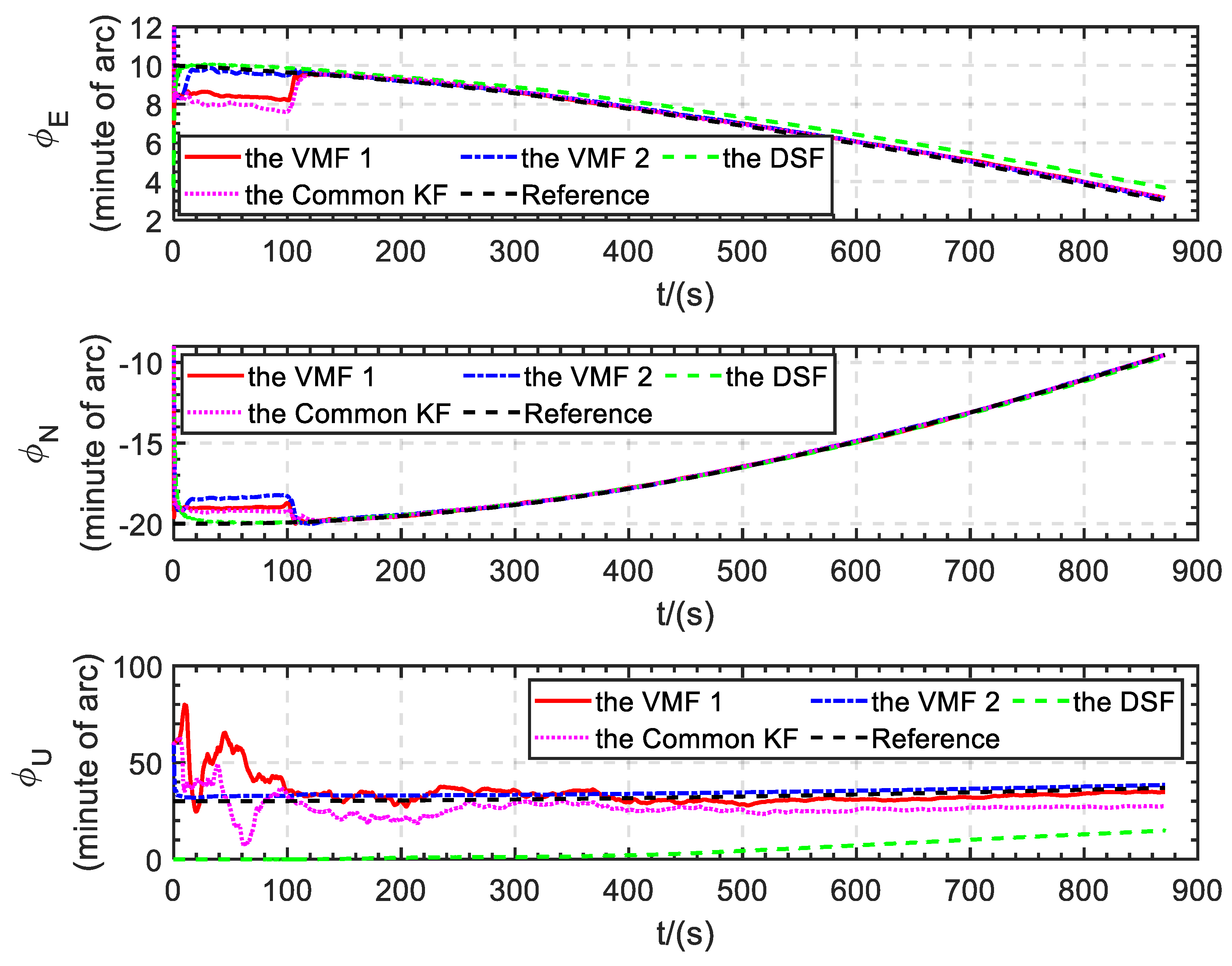
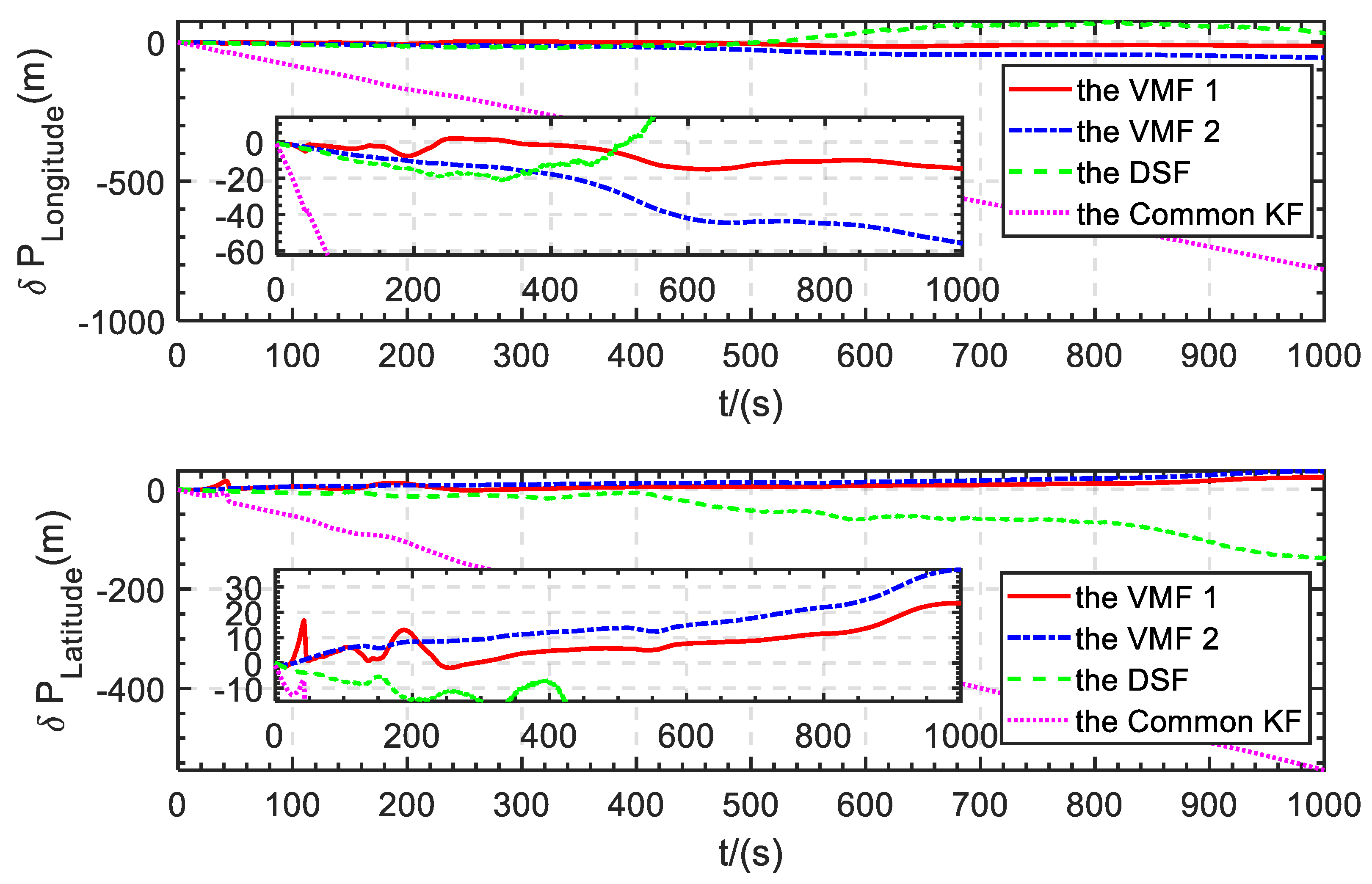
In addition, it can be seen from the new augmented measurement Equation (25) of VMF 1 that the velocity of DVL in the b-frame has been projected to the n-frame by the modified attitude matrix ${\widehat{\mathit{C}}}_b^n$, which has taken an approximate expression as ${\widehat{\mathit{C}}}_b^n(t_k)\approx \left[\mathit{I}+\left(\widehat{\mathit{\varphi }}(t_{k-1})\times \right)\right]{\mathit{C}}_b^{n^{\prime }}(t_k)$. In contrast, the new augmented measurement equation of VMF 2, Equation (32), did not involve the approximation of attitude information. Thus, the estimation capability of the attitude angle of the VMF 1 algorithm is weaker than that of VMF 2. Meanwhile, in the measurement equation shown in Equation (25), no error accumulated over time in the velocity measured by DVL in the b-frame. In contrast, the Equation (32) contains the accumulated SINS velocity error over time so that the VMF 1 has a better estimation capability for velocity than the VMF 2.

4. Simulation and Lake Test

4.1. Simulation Test

4.1.1. Simulation Test Setting

The simulation of mid-water is applied to verify the performance of the proposed Virtual Metrology Filters for estimating the constant ocean current velocity. The navigation trajectory of the AUV in the simulation test is shown in Figure 2 It moves along an approximate “8” trajectory in a horizontal plane at 50m underwater. The motion information, such as the attitude and the velocity, are shown in Figure 3. The initial attitude angles are [0 0 30] deg. The initial velocity is zero, and then the AUV accelerates to 5 m/s with the acceleration of 1 m/s², keeps 5 m/s for approximately 900 s, and finally decelerates to zero with the acceleration of −1 m/s².

Data from SINS, DVL, and PS are used during the algorithm validation process. The strapdown inertial navigation inversion algorithm generated the ideal angular velocity and acceleration values according to the trajectory. The output of the inertial measurement unit (IMU) is obtained by adding the bias and the random error to the ideal values as shown in

Table 1. The specifications of the inertial sensors and DVL error setting.

Items	Index	Values
Gyro	Bias	0.02 deg/h
	Angular Random Walk	0.0005 $\mathrm{deg}/\sqrt{\mathrm{h}}$
Accelerometer	Bias	50 μg
	Random Walk Noise	50 $\mathrm{\mu }\mathrm{g}/\sqrt{\mathrm{Hz}}$
DVL	Random Noise	0.2 cm/s

. Assuming that the velocity of the current is constant, regarding the velocity magnitude of the warm Kuroshio Current, it can be set as [0.5 0.8] m/s. The output of the DVL is the water-tracking velocity in the b-frame. It is constructed by removing the ocean current velocity from the ideal value of the velocity in the n-frame and projecting it into the b-frame, then adding some random noise, as presented in Equation (12). Depth information is provided directly by the PS. In addition, the installation error angle between SINS and DVL, and other errors, such as the scale factor of DVL, are assumed to have been well-calibrated before the simulation.

In the SINS/DVL integrated navigation system in which the error of velocity is selected as measurement quantities, the initial velocity and position errors cannot be corrected in the subsequent navigation process when no external sources provide absolute velocity and position information, so the initial velocity and position errors are set as zero in the simulation test. And it is assumed that the coarse alignment process has been operated before the simulation, and the initial misalignment angles are set as [10 −20 30] minute of arc. At the beginning of the algorithm validation, the initial iteration values are set as follows. The initial iteration values of the misalignment angle are set as [1 1 1] deg, the error of velocity is [0.1 0.1 0.1] m/s, the error of position is [1 1 1] m, the bias of the accelerometer are set as [500 500 500] μg, the bias of gyroscope is set as [0.05 0.05 0.05] deg/h, and the initial iteration of ocean current velocity are set as [0.1 0.1] m/s.

4.1.2. Results of the Simulation

To verify the effectiveness of the proposed VMF methods for estimating ocean velocities, we compared the velocity, attitude, and position errors obtained by the common KF and the DSF with those obtained by the VMF algorithms. The simulation results are as follows:

Figure 4 shows the velocity errors comparison in simulation test by the common KF, the DSF, the VMF 1, and the VMF 2, and their statistical characteristics are shown in

Table 2. Mean of velocity errors after 200 s in simulation test (m/s).

Index	The VMF 1	The VMF 2	The DSF	The Common KF
$\delta V_E$	0.0078	0.0135	0.0019	−0.5041
$\delta V_N$	−0.0071	−0.0117	−0.0371	−0.8010

. From Figure 4, we can see that the common KF method, which has ignored the velocity of the ocean current, has a velocity error close to the opposite of the ocean current. The DSF method has somewhat weakened the velocity error caused by ocean currents, but the velocity error still dissipates gradually with time. In contrast, the velocity errors of the two VMF methods proposed in this paper are close to zero. With the accumulation of velocity errors, the latitude and longitude errors of all four algorithms gradually diverged, as shown in Figure 5. And their statistical characteristics are shown in

Table 3. Max Position Errors in simulation test (m).

Index	The VMF 1	The VMF 2	The DSF	The Common KF
$\delta P_{Longitude}$	9.64	15.29	128.89	702.65
$\delta P_{Latitude}$	6.28	5.00	8.40	530.32
$\delta P$	10.34	15.29	128.91	880.32

. However, the position error of common KF is 1~2 magnitudes larger than that of the VMF methods. The maximum distance deviation is approximately 10.34 m for the VMF 1, 15.29 m for the VMF 2, and 128.91 m for the DSF. However, ignoring the effect of current velocity, the accumulation of velocity errors due to the current velocity results in a position error of 880.32 m in the common KF.

Figure 6 shows the misalignment angles comparison of the VMF 1, the VMF 2, the DSF, and the common KF. From Figure 6, the estimates of several methods for the eastward and northward misalignment angles overlap with the reference values. At the same time, VMF 1 and 2 with virtual measurements perform better than the common KF in estimating the upward misalignment angle. And, the DSF method has the largest misalignment angle.

There are four reasons for this: First, the two VMFs and the common KF methods can estimate the misalignment angles. Even if the ocean current velocity is coupled with the SINS velocity error, the misalignment angles’ observability is not affected according to (21), (31), and (38). Second, the velocity error and position error affect the misalignment angle estimation, which is determined by the misalignment angle differential equation. Thirdly, the upward misalignment angle is more vulnerable to velocity and position errors than the eastward and northward misalignment angles. Last, for the DSF, the coefficient in front of $\mathit{\varphi }$ is $\left({\mathit{C}}_b^n\Delta {\stackrel{⏜}{\mathit{V}}}_{DVL}^b\right)\times$, and the $\left({\mathit{C}}_b^n\Delta {\stackrel{⏜}{\mathit{V}}}_{DVL}^b\right)\times$ is a particularly small value, which makes $\mathit{\varphi }$ difficult to estimate.

Figure 7 shows the estimation of ocean current velocity in the simulation test by using the VMF 1, the VMF 2, and the DSF. It can be seen that the ocean current velocity converges quickly to the reference value. The reference value of the eastward current velocity is 0.5 m/s. The difference between the estimated and actual values of both VMF algorithms is controlled to be within 0.02 m/s. The reference value of the northward current velocity is 0.8 m/s. The difference between the estimated and actual values of both VMF algorithms is controlled to within 0.02 m/s. In comparison, the DSF method’s current velocity estimates are closer to the true value at the beginning and gradually deviate from the true value later on.

Figure 6 and Figure 7 show that the two VMF algorithms have advantages in misalignment angle and current estimation, respectively: the VMF 1 is closer to the reference for current velocity estimation, and the VMF 2 is closer to the reference for upward misalignment angle estimation. These simulation results are consistent with the analysis in Section 3.3.

Figure 8 shows the trajectory comparison using different simulation test methods. From Figure 8, we can see that the trajectories calculated by the VMF 1 and the VMF 2 coincide with the reference trajectory, while the trajectory of the common KF method has apparent significant “drift” which originates from the influence of the ocean current velocity on the trajectory calculation. And the trajectory of the DSF method has showed that it can eliminate the effect of ocean velocity to some extent, but the small offset still occurs.

4.2. Lake Test

4.2.1. Lake Test Setting

The lake test was completed on 8 July 2022 in Shazhou Lake, Zhangjiagang city, with the starting latitude and longitude coordinates [31.8887475 120.5594533] deg. The experimental devices are shown in Figure 9. The reference position information is provided by the global real-time kinematic (GRTK) positioning module of ArduPilot, and the angular acceleration and acceleration information are provided by the FN-120 IMU produced by Shaanxi Zhongke Qihang Technology Co., Ltd. Their main performance parameters are given in

Table 4. Main parameters of experiment devices.

	Items	Index	Values
GNSS	Single Point Positioning	Horizontal	0.4 m
		Vertical	2.5 m
	GRTK	Horizontal	1 cm + 1 ppm
		Vertical	1.5 cm + 1 ppm
	Sampling Rate		5 Hz
IMU	Gyro	Bias	<0.02 deg/h
		Angular Random Walk	<0.0005 $\mathrm{deg}/\sqrt{\mathrm{h}}$
	Accelerometer	Bias	<50 μg
		Random Walk Noise	<50 $\mathrm{\mu }\mathrm{g}/\sqrt{\mathrm{Hz}z}$
	Sampling Rate		100 Hz

. During the experiment, the data of all sensors are saved at the moment when the IMU data is coming to achieve the goal of time synchronization. During the experiment, although we used the DVL to obtain the speedboat’s velocity in the b-frame, the DVL was operating in bottom tracking mode. In order to verify the algorithm’s effectiveness under the existing experimental conditions in estimating the velocity of the current, we constructed the velocity that output of the DVL with the ocean current existed. The detailed construction is given in Equation (12).

The trajectory of the real lake test is similar to the simulation experiment, which is approximately in the shape of a number “8” as shown in Figure 10. Each side of the “8” is approximately 150 m, and the whole experiment lasted 1000 s. Unlike the previous simulation experiment, the truth value of the attitude, velocity, and position information is unavailable for the lake test. The motion information obtained by GNSS/SINS integrated navigation is used as the reference values for attitude, velocity, and position, as shown in Figure 10 and Figure 11. It should be noted that no GNSS position or speed information is used during the SINS/DVL integrated navigation. Throughout the navigation, there are ten turns each time the yaw angle is changed by approximately 90°. Meanwhile, the roll and pitch angles were almost zero, which indicates that the speedboat was only moving on the lake. In addition, the speedboat moves within a range of 2 m/s due to the limitations of the hooking components.

Similar to the simulation section, the ocean current is assumed constant and set as [0.5 0.8] m/s. The initial iteration values of the misalignment angle are set as [1 1 1] deg, the error of velocity is [0.1 0.1 0.1] m/s, the error of position is [1 1 1] m, the bias of the accelerometer are set as [50 50 50] μg, the bias of gyroscope is set as [0.01 0.01 0.01] deg/h, and the initial iteration of ocean current velocity are set as [0.1 0.1] m/s.

4.2.2. Results of Lake Test

Figure 12 shows the velocity errors comparison in the lake test, where we can see that the velocity errors of the common KF algorithm converge to the opposite values of the velocity of the ocean currents, with the eastward error approximately −0.5 m/s and the northward error approximately −0.8 m/s. Meanwhile, the velocity errors of the proposed two VMF methods converge near zero, and the velocity errors of the DSF method are small at the beginning and become larger with time subsequently. And

Table 5. Mean of velocity errors after 200 s in Lake Test (m/s).

Index	The VMF 1	The VMF 2	The DSF	The Common KF
$\delta V_E$	−0.0005	0.0127	−0.0750	−0.4945
$\delta V_N$	−0.0057	−0.0494	−0.3967	−0.8080

shows the statistical properties of the velocity errors after 200 s. The mean values in Table 5 are as analyzed above.

As time passes, the velocity errors accumulate into position errors, and the position errors of all four methods gradually diverge, as shown in Figure 13.

Table 6. Max Position Errors in Lake Test (m).

Index	The VMF 1	The VMF 2	The DSF	The Common KF
$\delta P_{Longitude}$	15.06	56.00	73.06	816.77
$\delta P_{Latitude}$	23.60	36.79	138.74	563.82
$\delta P$	27.81	67.00	143.42	992.48

shows the statistical characteristics of the position errors, from which it can be seen intuitively that the position errors of the proposed VMF methods are in a relatively small range, while the position error of the common KF have already moved away from the reference by a large magnitude, and the position error of the DSF method also gradually diverges.

Figure 14 shows the attitude errors comparison of different methods in the lake test. It shows that the Pitch and Roll errors of the different methods are relatively close and in a small magnitude, and it can be seen that the yaw error gradually converges to near zero after 200 s, with the exception of the DSF method. Figure 15 shows that the two VMF methods proposed in the paper are effective in estimating the velocity of ocean currents, with the estimated eastward and northward currents close to the set values and their maximum estimation errors not exceeding 0.05 m/s.

The results of the lake test are consistent with those of the simulation test, showing that the proposed VMF methods can alleviate the impact of constant currents on navigation and positioning in the SINS/DVL integrated navigation system, proving the effectiveness of the proposed methods.

5. Discussion and Conclusions

The ocean current velocity seriously affects the SINS/DVL integrated navigation ac-curacy. In this paper, we propose an innovative solution by formulating novel measurement equations within the structure of the Kalman filter. This strategy exploits the characteristic constancy of currents within small maritime regions over short durations. The two proposed Virtual Metrology Filters each exhibit specific advantages concerning the estimation of velocity and misalignment angle, respectively. These methods capitalize on historical data by leveraging state vector properties. The methods are characterized by an easily comprehensible model, high estimation accuracy, and importantly, independence from other external sensors.

However, this research is premised on the assumption of constant ocean current velocities within small maritime regions over short durations. Further research is necessary to address the complexities of vast long-term seas when relying on the SINS/DVL integrated navigation system. And due to experimental limitations, constructed ocean currents were employed in the lake test for algorithm validation. Future work should endeavor to conduct experimental verifications in genuine oceanic conditions.

References

1. Hegrenaes, O.; Hallingstad, O. Model-Aided INS With Sea Current Estimation for Robust Underwater Navigation. IEEE J. Ocean. Eng. 2011, 36, 316–337. [Google Scholar] [CrossRef]
2. Xu, B.; Wang, L.Z.; Li, S.X.; Zhang, J. A Novel Calibration Method of SINS/DVL Integration Navigation System Based on Quaternion. IEEE Sens. J. 2020, 20, 9567–9580. [Google Scholar] [CrossRef]
3. Liu, S.D.; Zhang, T.; Zhang, J.Y.; Zhu, Y.Y. A New Coupled Method of SINS/DVL Integrated Navigation Based on Improved Dual Adaptive Factors. IEEE Trans. Instrum. Meas. 2021, 70, 8504211. [Google Scholar] [CrossRef]
4. Liu, R.X.; Liu, F.C.; Liu, C.N.; Zhang, P.C. Modified Sage-Husa Adaptive Kalman Filter-Based SINS/DVL Integrated Navigation System for AUV. J. Sens. 2021, 2021, 9992041. [Google Scholar] [CrossRef]
5. Mu, X.K.; He, B.; Wu, S.Y.; Zhang, X.; Song, Y.; Yan, T.H. A practical INS/GPS/DVL/PS integrated navigation algorithm and its application on Autonomous Underwater Vehicle. Appl. Ocean. Res. 2021, 106, 102441. [Google Scholar] [CrossRef]
6. Ansari-Rad, S.; Hashemi, M.; Salarieh, H. Pseudo DVL reconstruction by an evolutionary TS-fuzzy algorithm for ocean vehicles. Measurement 2019, 147, 106831. [Google Scholar] [CrossRef]
7. Chang, L.B.; Di, J.B.; Qin, F.J. Inertial-Based Integration With Transformed INS Mechanization in Earth Frame. IEEE-ASME Trans. Mech. 2022, 27, 1738–1749. [Google Scholar] [CrossRef]
8. Chang, L.B.; Qin, F.J.; Xu, J.N. Strapdown Inertial Navigation System Initial Alignment Based on Group of Double Direct Spatial Isometries. IEEE Sens. J. 2022, 22, 803–818. [Google Scholar] [CrossRef]
9. Song, S.S.; Liu, J.; Guo, J.N.; Zhang, C.; Yang, T.T.; Cui, J.H. Efficient Velocity Estimation and Location Prediction in Underwater Acoustic Sensor Networks. IEEE Internet Things 2022, 9, 2984–2998. [Google Scholar] [CrossRef]
10. Qin, H.M.; Wang, Y.; Wang, G.C.; Qin, X.H.; Bian, Y.G. GSCV-XGBoost based information reconstruction and fusion method for SINS/DVL integrated navigation system. Meas. Sci. Technol. 2023, 34, 035105. [Google Scholar] [CrossRef]
11. Wu, Y.L.; Wang, X.S.; Zhao, Y.W.; Tang, Y.J. Research on SINS/DVL integrated navigation algorithm affected by ocean current. In AOPC 2020: Optical Sensing and Imaging Technology; CSOE: Xiamen, China, 2020; Volume 11567. [Google Scholar]
12. Li, D.; Xu, J.N.; Zhu, B.; He, H.Y. A calibration method of DVL in integrated navigation system based on particle swarm optimization. Measurement 2022, 187, 110325. [Google Scholar] [CrossRef]
13. Zhang, Y.S.; Guo, Y.J.; Yang, T.; Li, C.Y.; Wang, Z.Q. A novel separation and calibration method for DVL and compass error in dead reckoning navigation systems. Meas. Sci. Technol. 2016, 27, 065003. [Google Scholar] [CrossRef]
14. Luo, L.; Huang, Y.L.; Zhang, Z.; Zhang, Y.G. A New Kalman Filter-Based In-Motion Initial Alignment Method for DVL-Aided Low-Cost SINS. IEEE Trans. Veh. Technol. 2021, 70, 331–343. [Google Scholar] [CrossRef]
15. Xu, X.; Guo, Z.T.; Yao, Y.Q.; Zhang, T. Robust Initial Alignment for SINS/DVL Based on Reconstructed Observation Vectors. IEEE-ASME Trans. Mech. 2020, 25, 1659–1667. [Google Scholar] [CrossRef]
16. Wang, D.; Xu, X.S.; Yao, Y.Q.; Zhang, T.; Zhu, Y.Y. A Novel SINS/DVL Tightly Integrated Navigation Method for Complex Environment. IEEE Trans. Instrum. Meas. 2020, 69, 5183–5196. [Google Scholar] [CrossRef]
17. Batista, P.; Silvestre, C.; Oliveira, P. GAS ocean current estimation with limited velocity readings. IFAC Proc. Vol. 2012, 45, 337–342. [Google Scholar] [CrossRef]
18. Yao, Y.Q.; Xu, X.S.; Zhu, Y.Y.; Xu, X. In-motion coarse alignment method for SINS/DVL with the attitude dynamics. ISA Trans. 2020, 105, 377–386. [Google Scholar] [CrossRef]
19. Morgado, M.; Batista, P.; Oliveira, P.; Silvestre, C. Position USBL/DVL sensor-based navigation filter in the presence of unknown ocean currents. Automatica 2011, 47, 2604–2614. [Google Scholar] [CrossRef]
20. Wu, D.; Yan, Z.P.; Chen, T. Cooperative current estimation based multi-AUVs localization for deep ocean applications. Ocean. Eng. 2019, 188, 106148. [Google Scholar] [CrossRef]
21. He, K.F.; Liu, H.M.; Wang, Z.J. A Novel Adaptive Two-Stage Information Filter Approach for Deep-Sea USBL/DVL Integrated Navigation. Sensors 2020, 20, 6029. [Google Scholar] [CrossRef]
22. Meurer, C.; Fuentes-Perez, J.F.; Schwarzwalder, K.; Ludvigsen, M.; Sorensen, A.J.; Kruusmaa, M. 2D Estimation of Velocity Relative to Water and Tidal Currents Based on Differential Pressure for Autonomous Underwater Vehicles. IEEE Robot. Autom. Let. 2020, 5, 3444–3451. [Google Scholar] [CrossRef]
23. Saksvik, I.B.; Alcocer, A.; Hassani, V. A Deep Learning Approach To Dead-Reckoning Navigation For Autonomous Underwater Vehicles With Limited Sensor Payloads. In OCEANS 2021: San Diego–Porto; IEEE: Piscataway, NJ, USA, 2021. [Google Scholar]
24. Zang, X.L.; Ben, Y.Y.; Li, Q. INS/Log Integrated Navigation System with Ocean Current Velocity Model Based on Multiple Model Adaptive Estimation. In 2020 IEEE/ION Position, Location and Navigation Symposium (PLANS); IEEE: Piscataway, NJ, USA, 2020; pp. 817–821. [Google Scholar]
25. Sun, J.; Wang, F. An effective LS-SVM/AKF aided SINS/DVL integrated navigation system for underwater vehicles. Peer Peer Netw. Appl. 2022, 15, 1437–1451. [Google Scholar] [CrossRef]
26. Chang, D.; Johnson-Roberson, M.; Sun, J. An Active Perception Approach for Mid-Water Localization of Autonomous Underwater Vehicles. In 2020 American Control Conference (ACC); IEEE: Piscataway, NJ, USA, 2020; pp. 671–676. [Google Scholar]
27. Chang, D.; Johnson-Roberson, M.; Sun, J. An Active Perception Framework for Autonomous Underwater Vehicle Navigation Under Sensor Constraints. IEEE Trans. Control Syst. Trans. 2022, 30, 2301–2316. [Google Scholar] [CrossRef]
28. Liu, X.J.; Liu, X.X.; Shen, H.; Li, P.J.; Zhang, T.W. Self-aided SINS for spiral-diving human-occupied vehicle in midwater. Assem. Autom. 2021, 41, 106–115. [Google Scholar] [CrossRef]
29. Wu, X.Q.; Liu, X.X.; Wang, Z.X.; Huang, Y.J.; Sheng, G.R. A Self-Aided Strapdown inertial navigation method based on maneuver constraints and incremental observation. Measurement 2022, 201, 111763. [Google Scholar] [CrossRef]
30. Ben, Y.Y.; Zang, X.L.; Li, Q.; He, J.H. A Dual-State Filter for a Relative Velocity Aiding Strapdown Inertial Navigation System. IEEE Trans. Instrum. Meas. 2021, 70, 1000215. [Google Scholar] [CrossRef]
31. Wang, Z.X.; Liu, X.X.; Wu, X.Q.; Sheng, G.R.; Huang, Y.J. A virtual velocity-based integrated navigation method for strapdown inertial navigation system and Doppler velocity log coupled with unknown current. Rev. Sci. Instrum. 2022, 93, 065112. [Google Scholar] [CrossRef]
Figure 1. System structure of the common KF and VMFs for SINS/DVL integrated navigation system.
Remotesensing 15 04097 g001
Figure 2. The trajectory of the simulation test.
Remotesensing 15 04097 g002
Figure 3. The motion information for the simulation test.
Remotesensing 15 04097 g003
Figure 4. Velocity errors comparison in simulation test.
Remotesensing 15 04097 g004
Figure 5. Position errors comparison in simulation test.
Remotesensing 15 04097 g005
Figure 6. Misalignment angles comparison in simulation test.
Remotesensing 15 04097 g006
Figure 7. Estimation of ocean current velocity in simulation test.
Remotesensing 15 04097 g007
Figure 8. Trajectory comparison by using different methods in simulation test.
Remotesensing 15 04097 g008
Figure 9. Experiment device.
Remotesensing 15 04097 g009
Figure 10. The trajectory of the lake test.
Remotesensing 15 04097 g010
Figure 11. The motion information for the lake test.
Remotesensing 15 04097 g011
Figure 12. Velocity errors comparison in lake test.
Remotesensing 15 04097 g012
Figure 13. Position errors comparison in lake test.
Remotesensing 15 04097 g013
Figure 14. Attitude errors comparison in lake test.
Remotesensing 15 04097 g014
Figure 15. Estimation of ocean current velocity in the lake test by using the VMF 1, the VMF 2, and the DSF.
Remotesensing 15 04097 g015