A Cascade Network for Pattern Recognition Based on Radar Signal Characteristics in Noisy Environments

Abstract

Target recognition mainly focuses on three approaches: optical-image-based, echo-detection-based, and passive signal-analysis-based methods. Among them, the passive signal-based method is closely integrated with practical applications due to its strong environmental adaptability. Based on passive radar signal analysis, we design an “end-to-end” model that cascades a noise estimation network with a recognition network to identify working modes in noisy environments. The noise estimation network is implemented based on U-Net, which adopts a method of feature extraction and reconstruction to adaptively estimate the noise mapping level of the sample, which can help the recognition network to reduce noise interference. Focusing on the characteristics of radar signals, the recognition network is realized based on the multi-scale convolutional attention network (MSCANet). Firstly, deep group convolution is used to isolate the channel interaction in the shallow network. Then, through the multi-scale convolution module, the finer-grained features of the signal are extracted without increasing the complexity of the model. Finally, the self-attention mechanism is used to suppress the influence of low-correlation and negative-correlation channels and spaces. This method overcomes the problem of the conventional method being seriously disturbed by noise. We validated the proposed method in 81 kinds of noise environment, achieving an average accuracy of 94.65%. Additionally, we discussed the performance of six machine learning algorithms and four deep learning algorithms. Compared to these methods, the proposed MSCANet achieved an accuracy improvement of approximately 17%. Our method demonstrates better generalization and robustness.

1. Introduction

Radar is a necessary electronic device for most aerial targets. With the development of radar technology, airborne radar has come to possess multiple capabilities, such as aerial reconnaissance, target imaging, and firepower strikes. The radar working mode is a manifestation of its function. Radar mode identification (RMI) refers to the process of obtaining radar style and parameters from unknown electronic signals to analyze radar functions. Currently, people tend to pay more attention to the optical features and echo characteristics of the target, ignoring the passive microwave signal [1,2]. However, it should be noted that compared to optical and echo features, passive radar signals have three advantages [3,4,5]: (1) Signal reception is passive and has stronger stealth characteristics. (2) Radar signals are less affected by inclement weather such as rain, snow, and fog, making the signal more stable. (3) Radar signals can not only reflect the corresponding platform information, but also analyze the radar working mode to identify the target’s intention. Therefore, this paper focuses on passive radar signals to achieve the recognition of working modes, which can help to quickly identify target threats and be used to direct decision making. A scenario for its application is shown in Figure 1.

Nowadays, the impact of noise on signal processing is becoming more severe. In recent studies of working mode recognition [6,7,8], scenarios with stable environments and small parameter ranges have mainly been taken into account, but noise effects have not been fully considered. It is well known that noise has a significant impact on signals, especially for airborne radar. Strong noise can cause the loss and errors of pulses, directly changing the pulse repetition frequency and leading to identification errors. Under high-signal-to-noise ratio conditions, the signals are clear and the differences between working modes are apparent. A conventional deep learning network is capable of effectively extracting features for classification. Under a low signal-to-noise ratio, the following three challenges must be faced:

• Due to the uncertainty of scenarios, radar pulses may originate from different noise environments or different radars, and their parameter ranges are beyond the scope of “training data”, belonging to “unknown signals”. This seriously interferes with machine learning algorithms that are purely data-driven.
• As the signal-to-noise ratio decreases, a large amount of redundant or erroneous information will be mixed into the received radar pulses, resulting in the wrong parameters. At this point, the effective parameters cannot be determined, and originally traceable signals become chaotic.
• Defective radar signals differ from images in that the encoding and modulation styles of the signals are more diverse. The two types of inputs exhibit significant differences in terms of characteristics such as size, location, and shape. Noise has a more pronounced impact on signals, and conventional deep learning networks for computer vision are challenging to use to effectively process these differences. The comparison of a signal in an environment with significant noise is shown in Figure 2. It can be seen that the radar pulse pattern is difficult to distinguish under noise.

In this context, a dual-network cascade model based on latent-space noise encoding is proposed to address the aforementioned challenges. The main contributions of this paper are as follows:

• We employ a cascade learning approach with a noise estimation network and a recognition network, enhancing the algorithm’s adaptability in environments with strong noise.
• A noise estimation network based on U-Net is designed, which utilizes a symmetrical structure of upsampling and downsampling to extract and reconstruct noise features. The network achieves adaptive noise mapping relationships in different channels and spatial areas.
• The MSCANet, which is used to address the characteristics of radar pulse signals, is presented. The network is augmented with both deep-wise group convolution, multi-scale convolution, and self-attention mechanisms, which serve to improve the network’s feature extraction capabilities and make the model more lightweight.

The rest of this paper is arranged as follows. Firstly, we review the relevant work in the field of radar working mode recognition in Section 2. In Section 3, the proposed algorithm is introduced with regard to various aspects, including noise encoding in latent space, the group convolution method, multi-scale convolutional modules, and the self-attention mechanism. Section 4 reports datasets, experimental designs, and experimental results to evaluate and compare the performance of the proposed algorithm with other recognition technologies. Section 5 concludes this paper.

2. Related Work

Radar signal recognition can be mainly classified into traditional expert-knowledge-driven algorithms and data-driven algorithms represented by machine learning. With the diversification of radar systems and the complexity of electromagnetic space, traditional methods are gradually becoming ineffective, while data-driven algorithms have taken the lead in this field.

Data-driven methods optimize the known model by learning a large amount of data to achieve classification and recognition. In recent years, algorithms represented by deep learning have been widely used in computer vision, natural language processing, and other fields. The convolutional neural network (CNN) [9], recurrent neural network (RNN) [10], and self-attention mechanism [11] are three representative deep learning structures that each have advantages in radar signal recognition. Convolutional neural networks can extract the potential information of signals through feature mining; recurrent networks can preserve the semantic relationships; and self-attentive mechanisms are more advantageous in signal restoration. In practical scenarios, deep learning algorithms are usually limited by the following four aspects:

• Recognition of unknown signals. In [12,13], the authors propose a comprehensive recognition approach based on both traditional classifiers and deep learning networks. By utilizing the classifier to assist in network training, the central vectors of known data are deduced and thus the feasibility of recognizing unknown signals through known ones is verified.
• Few-shot learning problem. In [14,15], the authors explore model training methods under the conditions of few-shot learning by using the generated adversarial network and the auto-encoder embedded with the feature extraction module, respectively, solving the problem of a shortage of training data.
• Interpretability of recognition. This problem is a challenging research issue in various fields. From the perspective of integrating knowledge-driven and data-driven approaches, Refs. [16,17] have defined the feature representation of radar signals in deep learning networks, and have achieved embedded knowledge through prior knowledge assistance in network training.
• Low signal-to-noise ratio (SNR). It must be considered that SNR is a critical factor in the field of signal processing [18]. Reference [19] utilizes the characteristics of residual networks and adopts the naive method of deepening the network to improve recognition performance under a low SNR, with no further improvement possible after network saturation. In [20], the authors employ a fusion of CNN and the long short-term memory (LSTM) network to retain signal features and semantic relationships, but this method only focuses on short-term temporal dependencies and cannot extract global information. In [21], the authors propose a lightweight combinational neural network, which uses two networks for pre-recognition and fine recognition. The SEBlock attention module is embedded in the network to suppress noise interference. This method is suitable for multi-label classification tasks.

We specifically focused on the challenges posed by low-SNR environments in radiation source identification. Based on the aforementioned research, the main difficulty lies in extracting radar signal features in noisy environments. The above algorithms are essentially searching for differences among data, without considering the characteristics of radar signals. In other words, they are general methods in different fields, so their performance is significantly compromised when data are affected by noise.

Therefore, we propose a cascade network focusing on the characteristics of pulse signals in noisy environments. Among them, the noise encoding sub-network is built on the basis of U-Net. It is a classic network used for semantic segmentation in image processing, which has advantages in feature extraction and reconstruction due to its symmetric structure of upsampling and downsampling [22,23]. The recognition sub-network is an original design based on the characteristics of radar signals.

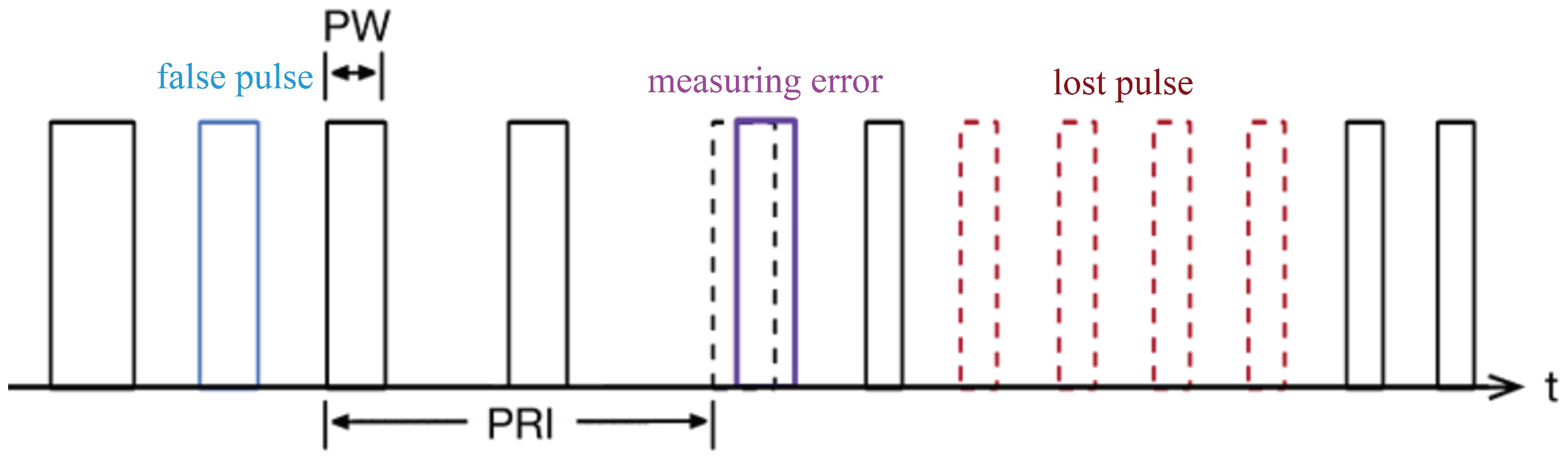
3. Radar Signal Detection in Noisy Environments

Firstly, the SNR problem needs to be transformed into a radar pulse detection problem. The target is detected when the signal intensity exceeds the threshold voltage $V_T$. Considering the relationship between $V_T$ and false alarm probability $P_f$, that is, $V_T=\sqrt{2{\psi }^2{ln}_{}1/P_f}$, the detection probability $P_d$ can be written as

$$P_d={\int }_{\sqrt{2{\psi }^2{ln}_{}1/P_f}}^{\infty }\frac{r}{{\psi }^2}{I}_0\left(\frac{Ar}{{\psi }^2}\right)exp\left(-\frac{r^2+A^2}{2{\psi }^2}\right)\mathrm{d}r$$

(1)

where $I_0\left(·\right)$ is the modified zero-order Bessel function. r and ${\psi }^2$ represent the modulus and variance of the noise, respectively. A is the echo amplitude.

When the noise follows a Gaussian distribution and $P_d$ is much larger than $P_f$, the A, r and $\psi$ in Formula (1) can be replaced by the signal-to-noise ratio (SNR), and the new formula can be approximated as follows:

$$P_d=0.5\times erfc\left(\sqrt{-{ln}_{}{P}_f}-\sqrt{SNR+0.5}\right)$$

(2)

with the following complementary error function $erfc\left(·\right)$:

$$erfc\left(x\right)=1-\frac{2}{\sqrt{\pi }}{\int }_0^x{e}^{-y^2}\mathrm{d}y$$

(3)

In summary, we can know that there will always be some loss or error radar pulse in noisy environments. The relationship between detection probability and SNR is shown in Figure 3.

Due to the interference of noise and the influence of hardware factors, a radar pulse will have some deviation, error and loss. Equation (2) shows that the detection probability, false alarm probability, and SNR are related. As the SNR decreases, the pulse distortion becomes more severe, and the probability of false alarms and missed detection increases. Therefore, for convenience of expression, we convert the impact of SNR on radar full pulses into lost pulses and false pulses, as shown in Figure 4. In the study of radar mode recognition, as a non-cooperative receiver, it is difficult to guarantee a certain false alarm probability and noise distribution. Therefore, adopting more intuitive lost pulses and false pulses instead of SNR is more reasonable. Based on the Robinson formula, the relationship between SNR and lost pulses can be approximately estimated. Under Gaussian conditions with 0 dB, the lost pulse rate is approximately 32%.

4. Algorithm Model and Implementation

4.1. Dual-Network Cascade Model

In this section, we designed an “end-to-end” recognition model with a dual-network cascade to address the problem of pulse pattern distortion in noisy environments. The model takes the full-pulse data from the radar as input and outputs the mode recognition result. Radar full-pulse data are a collection of pulse description words (PDW), which include radio frequency (RF), pulse width (PW), pulse amplitude (PA), direction of arrival (DOA), and time of arrival (TOA).

In radar signal processing, the receiver can observe the received signal from multiple dimensions, such as the radio frequency (RF), intermediate frequency (IF), base band, and full-pulse dimensions. Furthermore, according to the Fourier transform principle, feature extraction can be performed simultaneously from the temporal and spectral domains. For example, in reference [24], the signal is transformed into a spectrogram, resulting in continuity on the feature map, greatly enhancing the effectiveness of convolutional layers. However, it should be noted that mode recognition relies more on full-pulse data, which have more pronounced discreteness and weaker global self-correlation. As a result, noise more significantly disrupts the inherent pattern of the data, making conventional convolutional networks difficult to apply.

Therefore, we design the model in two parts. The first part is a noise estimation sub-network based on U-Net, which encodes the noise by downsampling and upsampling, and is used to adaptively estimate the sample’s noise level. The second part is a radar working mode recognition sub-network based on a multi-scale convolutional attention network, called MSCANet. It is trained using both the radar full-pulse and noise-coding information. The general diagram of the proposed scheme is shown in Figure 5.

Regarding the optimization of networks, we adopt a cascade approach to jointly train the noise estimation network and the classification recognition network to convergence, ensuring that both networks are optimized for the accurate identification of the working mode in noisy environments. At this point, the objective function of cascade training can be defined as the classification loss function:

$${\mathcal{L}}_c=-\frac{1}{N}\sum _{i=1}^N\left[y_i{ln}_{}{\widehat{y}}_i+\left(1-y_i\right){ln}_{}\left(1-{\widehat{y}}_i\right)\right]+\frac{\gamma }{2m}{\sum }_l^{}{\sum }_k^{}{\sum }_j^{}{\mathit{W}}_{\mathit{k},\mathit{j}}^{\left(\mathbf{l}\right)\mathbf{2}}$$

(4)

where $y_i$ represents the real label of N radar pulse samples within a batch size, and ${\widehat{y}}_i$ represents the prediction label. The second term of the formula is the regularization of the model, which is used to reduce the over-fitting phenomenon. The regularization coefficient $\gamma$ is set to 0.001, and ${\mathit{W}}_{\mathit{k},\mathit{j}}^{\left(\mathbf{l}\right)\mathbf{2}}$ represents the jth convolution kernel corresponding to the kth feature map in the lth layer.

4.2. Noise Estimation Network Based on U-Net

Due to the uncertainty of noisy environments, different signals are affected by noise to different extents. This irregular fluctuation is detrimental to recognition networks; therefore, a measure that can assess the level of signal noise is needed to help recognition networks filter out noise more effectively. In 2018, Ref. [25] first introduced the concept of noise level mapping into computer vision, and proposed FFDNet to help CNN complete image denoising and recognition. However, when the noise level of the evaluation is wrong, it will have a more adverse effect on the subsequent signal recognition. Therefore, in 2022, Du proposed a signal denoising classification network, DNCNet [18], from the point of view of signals. The algorithm pre-positioned a five-layer convolutional network to quantize the noise level, and then carried out denoising and identification. This method has a better dynamic evaluation ability for noise.

On the basis of the above research, we design a sub-network of hidden space noise coding, which needs to meet the following requirements:

• Each channel in the radar full pulse is affected by noise to different degrees, so it is necessary to evaluate the noise separately.
• The function describing the effect of noise on discrete radar pulses can be defined as an indicative function rather than a continuous function, so the whole sequence cannot be evaluated with a continuous mapping relationship.
• The purpose of noise evaluation is to help the classification network to recognize the working mode rather than to obtain certain information. The output noise coding sequence should match the input.

Based on the above requirements, we adopt the U-Net structure, whose symmetrical downsampling and upsampling can ensure that the output noise code is consistent with the input size. The coding point corresponds to the channel and time series in the pulse sequence. The process of sub-sampling can be regarded as the extraction of noise features, which consists of convolution and pooling. The upsampling process is to restore the original size according to the noise characteristics, which is realized by convolution and deconvolution. This progressive reduction structure can extract and recover information by gradually increasing the receptive field of the network, making it easier to grasp the noise features at different scales. The proposed noise estimation network is shown in Figure 6.

The input to the network is radar full pulses. The main structure consists of 16 convolutional layers, 2 deconvolution layers, and 2 average pooling layers. In order to preserve the independence of each channel during sampling, the network adopts one-dimensional convolution, pooling, and deconvolution. The kernel size is set to 3 × 1, and the number of kernels is 64, 128, and 256, in progressing order. The ReLU function is used as the activation function to correct the gradient. The change in the the feature map size is realized using the pooling layer and the deconvolution layer. Cascade pooling is adopted during downsampling; that is, the pooling size is greater than the step size, which can maintain the information interaction between adjacent data points. The output of the network is a noise coding matrix with the same size as the input, which can be used for the adaptive evaluation of the sample noise level.

Regarding the setting of hyperparameters, a layer-by-layer progressive structure is employed due to the symmetric nature of upsampling and downsampling. As for extracting noise features, the more convolutional kernels the network has, the stronger its expressive power. Therefore, incorporating more convolutional kernels is beneficial as long as the network does not overfit. In our tests, we found that the performance saturates when reaching 256 convolutional kernels in the middle layers. Hence, the structure shown in Figure 6 is employed for the network.

4.3. Recognition Network Based on MSCANet

According to the characteristics of radar pulses and the influence of noise, we design the following network structures in MSCANet. (1) Depth-wise group convolution. Independent convolution kernels are used for each channel in the shallow network. (2) Multi-scale 1D convolution. The multi-scale features of radar pulses are extracted using a convolution kernel of multiple parallel mutual primes. (3) Channel attention module (CAM) and spatial attention module (SAM). Adaptive weights of channels and spatial regions are implemented, enabling the network to focus on high-impact features. The structure of MSCANet is illustrated in Figure 7.

The network also employs global average pooling to replace fully connected layers and adopts residual structures to establish shortcut connections between modules. Deeper networks are more efficient in extracting features, while the above structures help to alleviate over-fitting in deep networks.

4.3.1. Depth-Wise Group Convolution

Radar pulse data are a set of discrete parameters in a time series, with no reliable correlations between channels. However, conventional convolution combines the feature maps of these channels, which is inefficient for extracting features from full-pulse data and results in substantial computational waste. Therefore, we adopt depth-wise group convolution to realize feature extraction.

Group convolution was first applied in AlexNet to solve the problem that a single GPU could not support simultaneous computation on feature maps. Therefore, the designers split the channels and computed them on separate GPUs. Subsequently, with the prevalence of lightweight networks, reference [26] combined group convolution with ResNet to propose the ResNeXt network. In comparison to contemporaneous networks such as Inception v4 and Inception-ResNet v2, the proposed model exhibits simpler and more lightweight architecture with equivalent recognition accuracy on the ImageNet dataset.

Using the same idea, we divide the pulse data into five groups, each group containing a dimension and the corresponding noise coding vector. The independent convolution kernel is used for feature extraction among the groups to ensure the independence of each channel in the shallow network. Channel concatenation is performed before the last convolution layer to preserve the correlation between channels. The specific structure is shown in Figure 8.

The advantage of depth-wise group convolution lies in not only isolating information interaction between different groups, but also reducing the computational complexity and parameter quantity to $1/5$ compared with conventional convolution. This makes the network more lightweight and faster.

Taking 1D convolution as an example in this paper, $C_{in}$ and $C_{out}$ represent the input and output channel number, respectively, K is the size of kernel, and the computational complexity of a kernel at a point for conventional convolution $O_1$ can be expressed as

$$O_1=C_{in}\times \left[K^2+\left(K^2-1\right)\right]+1=C_{in}\times \left(2K^2-1\right)+1$$

(5)

Then, the computational complexity of the entire convolutional layer is

$$O_c=C_{out}\times \left(O_1\times S_{out}\right)=C_{out}\times \left[C_{in}\times \left(2K^2-1\right)+1\right]\times S_{out}$$

(6)

where $S_{out}$ is the size of the output feature map. In the same way, the number of parameters for the convolution layer $P_c$ can be written as

$$P_c=C_{out}\times \left(C_{in}\times K+1\right)$$

(7)

When using depth-wise group convolution, assuming that the input feature map is split into g groups, the corresponding input and output feature map channels are reduced to $1/g$. Due to parallel calculations of g groups, this reduction is canceled out. However, corresponding to the change in the number of channels in the feature map, the number of channels in the convolution kernel also decreases to $C_{in}/g$. Therefore, the computational complexity $O_g$ and the number of parameters $P_g$ are expressed as

$$O_g=C_{out}\times \left[\frac{C_{in}}{g}\times \left(2K^2-1\right)+1\right]\times S_{out}$$

(8)

$$P_g=C_{out}\times \left(\frac{C_{in}}{g}\times K+1\right)$$

(9)

It is not difficult to see that the computational complexity and the number of parameters are reduced to approximately $1/g$ compared with conventional convolution, which proves the advantage of deep-wise group convolution.

4.3.2. Multi-Scale 1D Convolution

In the convolution layer, using kernels of the same size will compute the same region in the feature map. The difference between the kernels lies in their kernel parameters, but their receptive fields are the same. This is not conducive to adapting to pulse patterns under uncertain noise. Inspired by the application of short-time Fourier transform (STFT) with different window functions [27,28], we use parallel multi-scale convolution kernels instead of conventional kernels. By using the parallel computation of multi-scale convolutional kernels, the network has different “perspectives”, so it can extract more scale signal features when the number of convolutional kernels is the same. This idea is also reflected in the Inception network for image recognition [29]. Figure 9 shows the structure of the multi-scale convolution module.

In addition to using 1 × 1 convolutions to preserve the original feature map scale, the module adopts three types of 1D convolution kernel, with sizes of 3 × 1, 8 × 1, and 17 × 1, which are mutually prime. This design more efficiently extracts the fine-grained features of the original signal. Different-scale convolution kernels are equivalent to mapping feature values at different window sizes. Thus, the mapping $z_{ij}^{xy}$ of the ith layer and jth feature map at location $\left(x,y\right)$ can be expressed as

$$z_{ij}^{xy}=f\left(\sum _{k=1}^K\sum _h^{H_m-1}\sum _w^{W_m-1}{\omega }_{ijk}^{hw}{z}_{\left(i-1\right)k}^{\left(x+h\right)\left(y+w\right)}+b_{ij}\right)$$

(10)

where K is the number of feature maps at the $i-1$ layer, $H_m\times W_m$ is the size of the convolution kernel, ${\omega }_{ijk}^{hw}$ is the convolution kernel parameter matrix connected to the kth feature map at $i-1$ layer, $b_{ij}$ is the bias, and $f\left(·\right)$ is the ReLU activation function. We write the matrix of $z_{ij}^{xy}$ as $\mathit{F}$, and then the output feature map is

$${\mathit{F}}^{\mathbf{\prime }}=Concat\left(\mathit{F}\ast {\mathit{V}}_{\mathbf{1}},\mathit{F}\ast {\mathit{V}}_{\mathbf{2}},\mathit{F}\ast {\mathit{V}}_{\mathbf{3}},\mathit{F}\ast {\mathit{V}}_{\mathbf{4}}\right)$$

(11)

where $Concat$ is a operation of channel concatenation. Different from the pyramid-type feature maps obtained by conventional convolution, multi-scale convolution can obtain more receptive fields of different sizes and with richer feature levels.

4.3.3. Self-Attention Mechanism

The influence of different parameters and regions on the operating modes in radar pulses varies greatly, but convolution is local and indiscriminate. Therefore, it is necessary to adopt different selection strategies. In order to extract signal features with emphasis and preserve semantic relationships, we introduce the channel self-attention module (CAM) and spatial self-attention module (SAM) to achieve adaptive weight allocation, enabling the network to pay more attention to valuable channels and regions [30].

The structure of CAM is shown in Figure 10. First, parallel maximum pooling and average pooling are utilized to compress the feature maps along the spatial dimensions, yielding channel-wise vectors and resulting in two $1\times 1\times C$ feature maps, where C represents the number of channels, and H and W represent the height and width of the feature map, respectively. Then, the obtained feature maps are input into a shared two-layer perceptron, with a ReLU activation function in between, and the number of neurons in the second layer is equal to the number of output channels, which enhances the trainability of CAM. Finally, an element-wise operation is applied to the two kinds of pooling graphs, and the output feature map ${\mathit{M}}_{\mathit{c}}$ is written as

$${\mathit{M}}_{\mathit{c}}\left(\mathit{F}\right)=f\left({\mathit{W}}_{\mathbf{0}}\otimes {\mathit{W}}_{\mathbf{1}}\otimes {\mathit{F}}_{\mathit{avg}}^{\mathit{c}}+{\mathit{W}}_{\mathbf{0}}\otimes {\mathit{W}}_{\mathbf{1}}\otimes {\mathit{F}}_{\mathit{max}}^{\mathit{c}}\right)$$

(12)

where $f\left(·\right)$ is the sigmoid activation function, ${\mathit{W}}_{\mathbf{0}}$ and ${\mathit{W}}_{\mathbf{1}}$ are the weight vectors of the two-layer shared perceptron, and ⊗ is the Kronecker product. ${\mathit{F}}_{\mathit{avg}}^{\mathit{c}}$ and ${\mathit{F}}_{\mathit{max}}^{\mathit{c}}$ represent the global average pooling and global maximum pooling, respectively. The two pooling operations ensure that the model generates feedback on the global region and maximum region of the feature map, so the performance is better than that of SENet [31], which uses only average pooling.

The structure of the SAM is shown in Figure 11. SAM is calculated on the basis of CAM; the module compresses the channel information and retains the attention paid to the spatial information. Firstly, global average pooling and global maximum pooling based on the channel dimension are used to calculate feature maps. After splicing into $H\times W\times 2$ feature maps, the average pooling and maximum pooling information are extracted by 3 × 1 convolution, and the feature maps are again reduced to one dimension. The expression for ${\mathit{M}}_{\mathit{s}}$ is as follows:

$${\mathit{M}}_{\mathit{s}}\left(\mathit{F}\right)=f\left(Con{v}_{1D}^3\left[{\mathit{F}}_{\mathit{avg}}^{\mathit{s}},{\mathit{F}}_{\mathit{max}}^{\mathit{s}}\right]\right)$$

(13)

where $Con{v}_{1D}^3$ is the 1D convolution of 3 × 1, and ${\mathit{F}}_{\mathit{avg}}^{\mathit{s}}$ and ${\mathit{F}}_{\mathit{max}}^{\mathit{s}}$ represent global average pooling and global maximum pooling, respectively.

Furthermore, multi-scale convolution is used to obtain more multivariate feature maps, which better improves the performance of the self-attention mechanism. The CAM enables the network to focus on more efficient feature maps in multi-scale convolution, such as the local information of modulation laws. The SAM can filter out the information redundancy or area of error caused by interference at different sizes. All of these features can help the network to improve the recognition performance under significant noise.

5. Experiments and Results

In this section, the effectiveness of the proposed algorithm in significantly noisy environments is demonstrated through simulation experiments, which include four parts:

• Considering different application scenarios, 10 kinds of typical radar working modes are constructed for the demonstration of subsequent experiments.
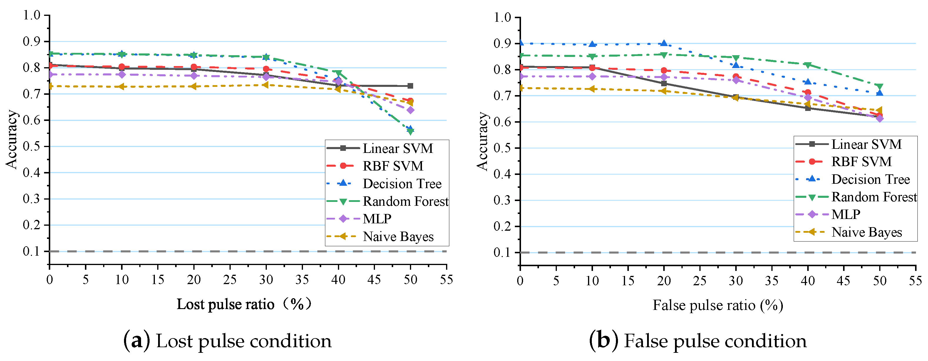
• The performance of traditional machine learning algorithms and deep learning algorithms is tested to prove the limitations of conventional artificial intelligence algorithms in noisy environments.
• By introducing the noise estimation sub-network, the performance of the single classification model and dual-network cascade model is compared.
• The performance of the proposed MSCANet network is compared with that of the classical deep learning network, and the influence of noise on the radar working mode is analyzed.

5.1. Dataset

Due to the confidentiality of radar parameters, no public dataset is available at present. Therefore, on the basis of the public literature [6,32,33] and referring to authoritative books such as Radar Manual, Airborne Radar Manual, and Pulse Doppler Radar, we simulated and constructed a radar full-pulse dataset, namely RPDWS-I, which covers the typical modes of reconnaissance, search, tracking, moving target indication, and SAR.

The dataset includes the following 10 kinds of radar working modes: Velocity Search (VS), Range While Search (RWS), Velocity-Range Search (VRS), Multiple-Target Tracking (MTT), Beam Riding (BR), Ground Moving Target Indication (GMTI), Ground Moving Target Tracking (GMTT), Sea Surface Search (SSS), Sea Surface Tracking (SST), and Synthetic Aperture Radar (SAR). The training set includes 4000 samples for each model. The test set has a total of 81 test environments, and the range of missed pulses and false pulses is set to 0∼80%. The interval is 10%, with 1000 samples for each environment. In order to present the experimental results succinctly and clearly, the baseline algorithm only tests the model performance under 0∼50% lost pulse and false pulse environments, and the proposed algorithm is tested under all environments. The signal parameters in the dataset are shown in

Table 1. RPDWS-I dataset. Each working mode sample is random within the given range to simulate uncertain radar parameters.

Working Mode	PRI (us)	PW (us)	Duty Ratio (%)	Pulse Num in CPI	Bandwidth (MHz)	Modulation
VS	3.3∼10	1∼3	10∼30	500∼2000	0.3∼10	Consatnt
RWS	3.3∼10	1∼3	10∼30	500∼2000	0.3∼10	D&S
VRS	50∼165	1∼20	1∼25	30∼256	1∼10	Constant, D&S
MTT	3.3∼125	0.1∼20	0.1∼25	1∼64	1∼50	Stagger, Sliding
BR	3.3∼125	0.1∼20	0.1∼25	1∼64	1∼50	Wobbulated
GMTI	120∼500	2∼60	0.1∼25	20∼256	0.5∼15	Stagger
GMTT	62∼160	2∼40	0.1∼25	20∼256	0.5∼15	Stagger
SSS	1000∼2000	1∼200	0.1∼10	1∼8	0.2∼500	Stagger
SST	500∼1000	1∼200	0.1∼20	20∼256	0.2∼10	Stagger
SAR	100∼1000	3∼60	1∼25	70∼20,000	10∼500	Constant

, and the following parameter range and modulation style are confirmed in [34].

5.2. The Performance of Traditional Radar Target Recognition Algorithms

Traditional radar signal recognition methods are mainly based on statistical analysis and inference. In the current environment with complex radar signal patterns and dense interference signals, these methods have become less applicable. This paper tests three classic recognition algorithms, including the PRI transformation method, syntactic model method, and Bayesian inference method. The PRI transformation method extends the radar pulse arrival time autocorrelation sequence to the frequency domain, and identifies radar signals under ambiguous matching conditions. The syntactic model method decomposes radar signals into hierarchical levels, such as radar words, phrases, sentences, and paragraphs, and then models them layer by layer to represent radar signals. It identifies targets based on their interrelationships. The Bayesian inference method employs conditional probability to infer radar signals layer by layer. The recognition results of the three methods are shown in Figure 12.

Traditional radar target recognition algorithms rely on the accuracy of intercepted signals. When interference from noise reduces the effective pulses below a critical threshold, the recognition capability significantly declines. As seen from Figure 12, all three algorithms demonstrate excellent recognition abilities in an ideal environment. However, when noise is introduced, all three methods are noticeably affected and reach a critical point at approximately 20% interference pulse ratio, with PRI transformation method showing the most severe performance degradation. A comparison between Figure 12a and Figure 12b reveals that false pulses have a greater impact than missed pulses. This is because false pulses introduce erroneous information, interfering with the algorithm’s recognition process, whereas missed pulses represent the loss of valid information, resulting in less interference. These results indicate that under significant noise conditions, traditional radar target recognition methods become less applicable.

5.3. The Performance of Conventional Artificial Intelligence Algorithms

Conventional artificial intelligence algorithms learn radar signal features in noisy environments by using noise samples. Therefore, we randomly select 20% of the samples in the training set, and successively add a 10∼30% ratio of the lost and false pulses as a data enhancement measure to help the classifier to extract data features in a noisy environment.

5.3.1. Traditional Machine Learning Algorithms

We selected six kinds of widely used machine learning classifiers for validation, as follows:

Linear support vector machine (SVM). The classifier uses the linear kernel as a mapping function, which has the best effect in linearly separable datasets. However, features of the radar full pulse include high-dimensional data and being linearly indivisible, which cannot meet the requirements. Therefore, the model should have a certain tolerance for misclassification, with the penalty factor C set at 0.025. The SVM classifier is trained with the aforementioned hyperparameter settings, and the training samples are standardized before inputting them into the classifier. As mode recognition is a multi-class problem, this study employed a multi-class SVM as the loss function, and the optimization algorithm is the gradient descent method.

Radial basis function (RBF) SVM. The classifier uses the Gaussian kernel as a mapping function, which is suitable for high-dimensional and linearly inseparable full-pulse features. Therefore, the focus of the research is to improve the recognition accuracy and avoid incorrect classification. The standard deviation of the kernel parameter $\sigma =0.01$, and the penalty factor $C=1$. The training process is consistent with the linear SVM classifier mentioned earlier.

Decision tree. In the algorithm, the data are divided by splitting the dataset down into smaller sets, the number of splits being equal to the depth of the decision tree. In this paper, the Gini coefficient is used as the decision condition for dividing the node dataset. “Node” contains at least two samples, “leaf” contains at least one sample, and the maximum depth is 5. During training, the data are first standardized and then input into the decision tree for node splitting. Subsequently, starting from the root node, the entire decision tree is constructed recursively based on feature selection and stopping criteria. Finally, pruning is performed to determine the final model.

Random forest. The algorithm is based on the Bagging ensemble learning method, which divides the dataset into multiple random subsets, trains it on multiple base models, and finally achieves the classification result by “voting”. Therefore, the algorithm can better eliminate the bias of a single model and prevent overfitting. In the algorithm, the base model is the decision tree classifier mentioned above, and the number of base models is 100. The same optimization method as mentioned earlier for decision trees is used, but with the addition of a voting mechanism involving multiple decision trees.

Multi-layer perceptron (MLP). As an early neural network, the MLP is mainly composed of fully connected layers. The network consists of three layers: the input layer, hidden layer, and output layer. The number of neurons in the input layer is equal to the number of features in the samples, while the number of neurons in the output layer corresponds to the kinds of recognition modes. The hidden layer comprises 1000 neurons. The ReLU function is utilized as the activation function, and the optimizer employed is Adam. A batch size of 200 is utilized, and a total of 200 iterations are conducted.

Naive Bayes. Based on Bayes’ theorem, the posterior probability of classification is obtained by calculating prior probability, marginal likelihood estimation, and likelihood estimation. The algorithm does not need to perform iterative calculation and has no preset parameters, which is suitable for large datasets. During training, the prior probabilities of each recognition mode in the training set are calculated, and then conditional probabilities are estimated based on the features. The final model is obtained by saving these probabilities.

According to the above parameter settings, the performance of the classifiers is tested under different proportions of lost and false pulses. The results are shown in Figure 13. The gray dashed line represents the invalid recognition line. The average accuracy of six classifiers—linear SVM, RBF SVM, decision tree, random forest, MLP, and naive Bayes—in identifying radar operating modes in a 0∼50% lost pulse environment is 77.2%, 77.3%, 78.4%, 78.9%, 74.5%, and 71.2%, respectively. In a 0∼50% false pulse environment, the average accuracy is 72.2%, 75.3%, 82.8%, 82.6%, 73.1%, and 69.6%, respectively. When the interference pulse ratio is below 30%, the recognition accuracy of the aforementioned classifiers remains relatively stable, but it significantly declines after exceeding 30%.

The results show the following: (1) The overall recognition accuracy of the classifiers is not high, and the representation ability of traditional machine learning classifiers is not enough to support the extraction of radar features. (2) There is little difference in recognition ability between the two environments, and the classifier cannot take specific anti-interference measures for different environments. (3) The classifier relies heavily on the data distribution of the training set, and the recognition performance deteriorates significantly after it exceeds the range.

5.3.2. Conventional Deep Learning Algorithms

We selected four kinds of classic convolutional networks for testing, which have won championships in the ILSVRC competition and have been successfully applied in the field of radiation source identification. These models are ConvNet [12], ResNet [24], AlexNet [35], and VGGNet [36]. Among them, ResNet adopts the same basic structure as MSCANet, and the structures of ConvNet, AlexNet, and VGGNet are shown in Figure 14. To adapt to the radar pulse dataset, all convolution and pooling operations in the above networks are adjusted to 1D. The networks use the Adam optimizer, and the learning rate decreases from ${10}^{-2}$ to ${10}^{-4}$ every 40 epochs. The batch size is set to 256, and each training consists of 160 epochs. The networks are regularized by L2 regularization with a value of ${10}^{-4}$.

The ConvNet, AlexNet, and VGGNet directly adopt the structures provided in references [12,35,36], without parameter adjustment or optimization. For ResNet, the depth is reduced to 18 layers from the original architecture, and the size and quantity of convolutional kernels are optimized. This is achieved based on three main considerations:

• Through experiments, we found that optimizing ResNet only resulted in an approximate 4% improvement in recognition accuracy, and the trend of accuracy change with varying lost pulses remained largely unchanged, indicating limited impact.
• Other networks using their original structures could validate that classic image recognition networks are not directly applicable to radar pattern recognition in noisy environments.
• When evaluating the performance of the noise estimation sub-network, using the optimized ResNet, as well as the original ConvNet, AlexNet, and VGGNet as baseline models, can provide more comprehensive results.

We conducted experiments in the same environment to test the deep learning algorithms. The accuracies of the four algorithms on the training set are shown in

Table 2. Accuracy of deep learning networks in the training set.

AlexNet	ConvNet-18	ResNet-18	VGGNet
96.9%	90.7%	90.5%	99.7%

, all of which are above 90%. However, the performance of the networks on the test set is unstable, as shown in Figure 15.

It can be observed that AlexNet and ResNet-18 have better overall accuracy than ConvNet-18 and VGGNet, but this is still lower than the accuracy on the training set. All four networks exhibit a certain degree of overfitting. Although ConvNet-18 and VGGNet have deeper network structures compared to AlexNet, they lack effective measures to alleviate overfitting, resulting in worse test results. Deeper network structures can make the output closer to the training set, but it may not be effective for the test set. Although ResNet-18 also adopts a deep network structure, its residual connections help the network alleviate the overfitting problem.

A more concerning phenomenon is that the test accuracy of the four networks does not monotonically decrease but instead exhibits “peaks” at different positions. Due to the interference pulse ratio added in the training data ranging from 10% to 30%, when the test data have a similar distribution to the training data, the accuracy is relatively high, but the recognition ability declines in an ideal environment without interference. This means that the above four networks have not “learned” the true characteristics of the radar working mode, but are instead fitted to the data distribution in the training set.

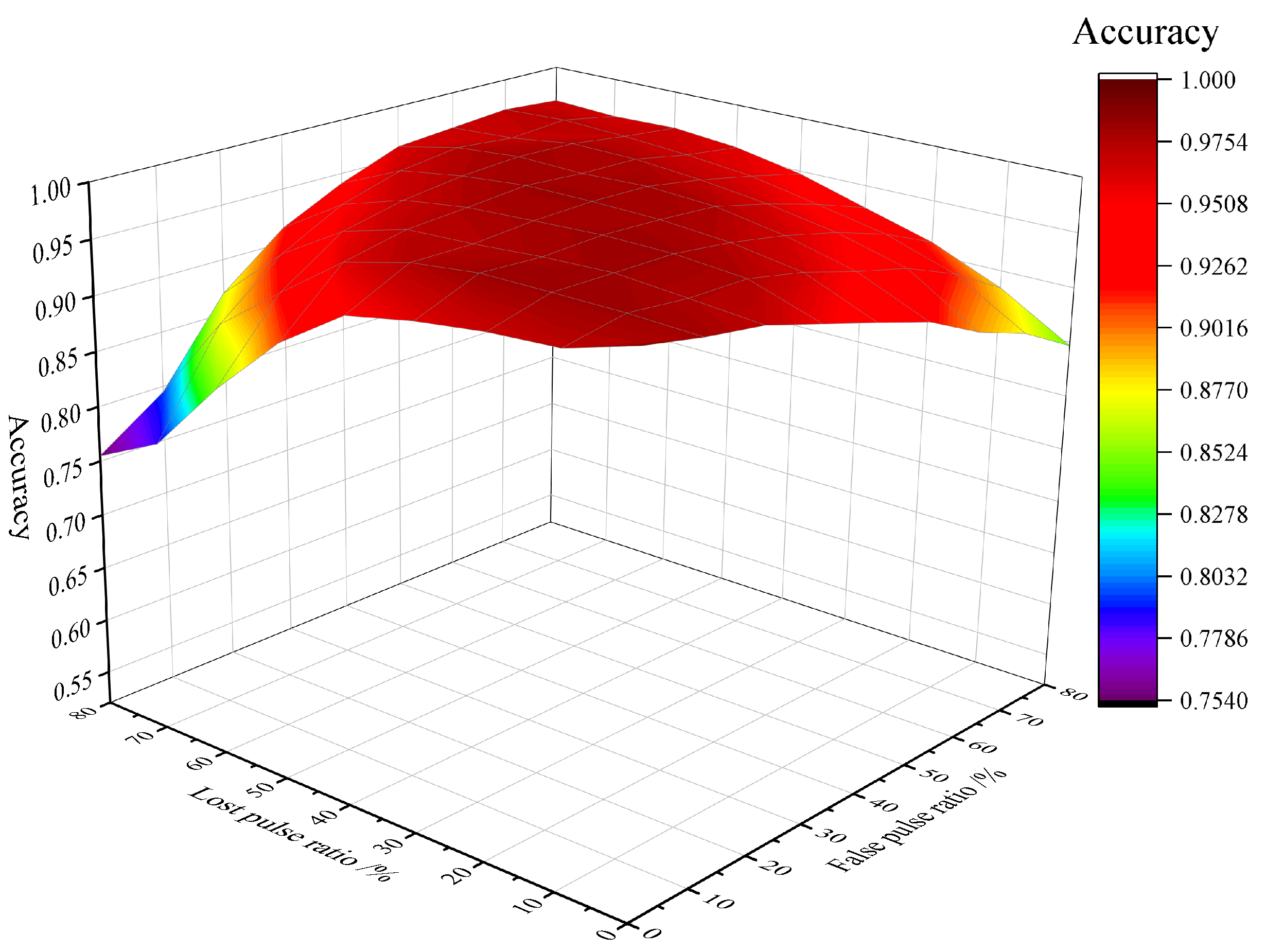
5.4. The Performance of the Proposed Noise Estimation Sub-Network

In order to verify the performance improvement brought about by adaptive noise coding, we first introduce noise estimation sub-networks in different noise environments for testing. The model which combines the noise estimation sub-network and classification recognition network is called the “cascade model”, and the single recognition network is denoted as the “independent model”. This part of the experiment compares the recognition accuracy of the two kinds of models. The baseline models consist of ConvNet-18, AlexNet, VGGNet, and ResNet-18, which are mentioned above. To match the noise estimation sub-network, the cascade models all adopt deep-wise group convolution.

The results are shown in Figure 16. Compared with the independent model, the average recognition accuracy of the cascade models is improved by 10∼30%. The fluctuation of recognition accuracy in different test environments is further reduced. The more the noise affects the model, the more the recognition rate improves after the introduction of the noise estimation sub-network. This fully demonstrates that adaptive noise estimation can help recognition models to reduce noise interference.

5.5. The Performance of Proposed MSCANet

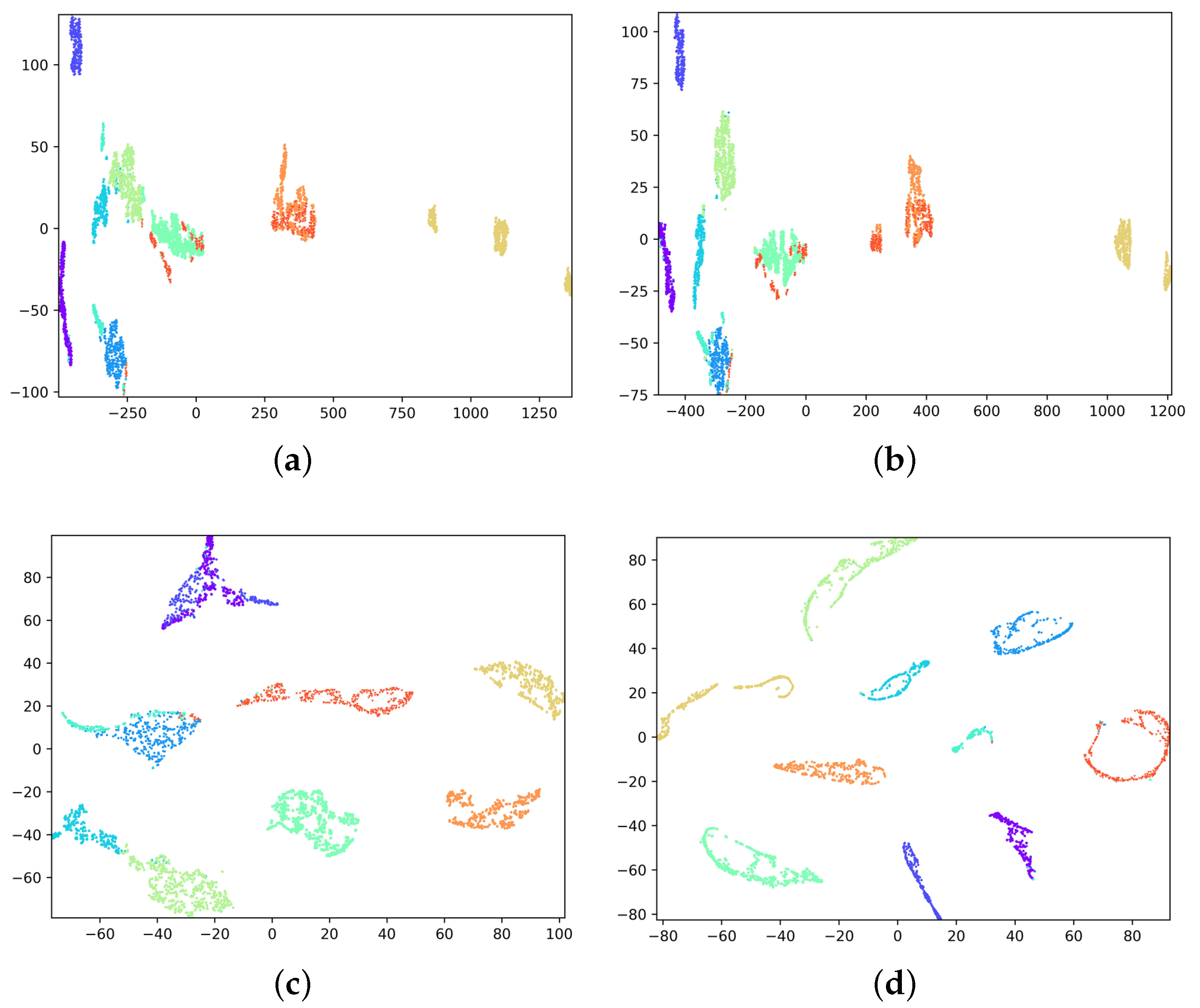
5.5.1. In-Training Views

MSCANet uses the same training conditions as the conventional deep learning networks described above. The Adam optimizer is used, and the learning rate decreases from ${10}^{-2}$ to ${10}^{-4}$ every 40 epochs. The batch size is set to 256, and each training iteration consists of 160 epochs. The networks are regularized by L2 regularization with a value of ${10}^{-4}$. The network is trained 10 times to ensure stability. The results are shown in Figure 17.

It can be seen that MSCANet exhibits fast and stable convergence. After the 120th epoch with the learning rate decreased to ${10}^{-4}$, the accuracy of the training set and validation set aligns, demonstrating superior convergence performance. Additionally, the fluctuations in the training curve at the 40th, 80th, and 120th epoch are normal, since the learning rate undergoes changes at these points.

5.5.2. MSCANet Recognition Performance

To demonstrate the recognition performance of MSCANet in complex environments, this part of the experiment extends the ratio of lost pulses and false pulses to 0∼80%. The three-dimensional surface of recognition accuracy is shown in Figure 18.

Under different ratios of missed pulses and false pulses, MSCANet achieves an average recognition rate of 94.65%, and the surface of test accuracy is relatively flat, indicating stable recognition capability. In an ideal environment, the network achieves the highest recognition accuracy of 98.46%, which indicates that the network truly extracts recognition features from radar pulse patterns. It should be noted that the model is not immune to the interference of error terms, but in comparison to the baseline network, MSCANet demonstrates stronger anti-interference capabilities.

To validate the performance improvement of the proposed MSCANet,

Table 3. Recognition accuracy of several networks in different environments.

Model	Lost Pulse Ratio (%)						False Pulse Ratio (%)						Process Time (s)	Model Capacity
	0	10	20	30	40	50	0	10	20	30	40	50
AlexNet	70.4	70.3	76.4	81.5	88.1	90.2	70.9	83.6	90.7	93.2	95.0	93.6	2.42	520 K
ConvNet-18	65.2	73.5	76.6	82.8	92.1	88.3	65.2	66.8	71.3	77.3	86.9	86.1	11.46	954 K
ResNet-18	79.1	84.2	87.7	89.3	89.4	87.5	79.1	85.6	90.3	90.2	88.4	86.1	11.93	1110 K
VGGNet	68.0	92.3	88.7	82.8	81.7	80.1	68.1	89.2	88.2	86.9	84.7	80.3	9.15	1680 K
MSCANet	98.4	97.8	97.5	97.1	96.2	94.3	98.4	97.8	97.1	95.4	93.7	92.1	14.50	849 K

provides a comparison of different networks under conditions of lost pulses and false pulses. The experiments were run on JetBrains PyCharm 2022 with an Intel (R) Core (TM) CPU i7-9900k@4.20 GHz and an NVIDIA GeForceRTX2060 GPU. It can be observed that (1) MSCANet achieves an average accuracy improvement of 5% to 20% compared to other networks; (2) except for AlexNet and MSCANet performing similarly under 40% and 50% false pulse conditions, MSCANet exhibits the best recognition performance in other environments; and (3) MSCANet overcomes the issue of model overfitting, and the recognition accuracy decreases slowly as the environment deteriorates.

To visually demonstrate the feature extraction capability of the network, the output feature maps of the last convolutional layer in the pre-trained AlexNet, VGGNet, ResNet-18, and MSCANet models are extracted for the same test samples. Principal component analysis (PCA) is used for dimensionality reduction and visualization, and the results are shown in Figure 19.

It can be observed that the AlexNet and VGGNet samples are scattered and unevenly distributed, making them prone to confusion. The inter-cluster distance of ResNet-18 is relatively large, but there is overlap among some samples, resulting in incomplete classification. The results generated by the proposed MSCANet in this paper exhibit a neat distribution of the 10 classes, with strong intra-cluster aggregation and large inter-cluster distances. Therefore, it can be concluded that the proposed method outperforms other baseline models in the UAV radar working mode recognition task.

5.5.3. Ablation Study

To further demonstrate the necessity of the deep group convolution, multi-scale convolution, and self-attention mechanism proposed in this paper, a set of ablation experiments is conducted to evaluate the network performance under different structures. Additionally, the performance improvement brought about by noise encoding has been proven in the previous part and will not be reiterated here. This set of experiments is divided into four groups: (1) the complete structure of MSCANet; (2) the network without the deep-wise group convolution structure, referred to as “without GC”; (3) a network without the multi-scale convolution and self-attention mechanism, referred to as “without CA”; and (4) a conventional convolutional network without the above design structures, which degenerates into the initial deep residual network, referred to as “ResNet-initial”.

Taking the lost pulse environment as an example, the results are shown in Figure 20. It can be observed that, except for the “ResNet-initial” network, the other three networks with designed structures in this paper exhibit more stable recognition under different environments, and their recognition curves show a monotonically decreasing trend, which aligns with objective cognition. In terms of accuracy analysis, the average accuracy of the four structures is 96.9%, 85.0%, 84.4%, and 78.7%, respectively. MSCANet has a significantly higher recognition capability than the other three networks. “Without GC” has slightly higher accuracy than “without CA”. “ResNet-initial” has the lowest accuracy.

6. Discussion

In this paper, to address the problem of radar mode recognition in high-noise environments, we proposed a dual-network cascade model. The effectiveness of the proposed method is validated in 81 different noise environments. Our noise estimation sub-network effectively mitigates noise interference through adaptive noise coding. With the assistance of this structure, the proposed MSCANet is more suitable for feature extraction in radar pulse signals. This work is a further improvement compared with the latest research [13,37] on radar working mode recognition.

Under the same signal processing approach, deep learning models, such as ConvNet, ResNet, AlexNet, and VGGNet, are superior to traditional machine learning classifiers, but the transferability of the algorithms in different noise environments is poor. We observed over-fitting on the test set through experiments. Taking VGGNet as an example, the recognition rate exhibits a clear peak as the noise increases, indicating that the network only matches the signal data distribution at the peak points. The addition of noise causes a single recognition model to fit the erroneous data with superimposed noise, failing to learn the true characteristics of the signal. Therefore, although it possesses some recognition ability, it cannot meet the practical requirements in terms of recognition accuracy and environmental adaptability.

Deep learning models have strong feature representation capabilities, but due to the uncertainty of noise, these models tend to exhibit varying degrees of over-fitting. Therefore, we designed a noise estimation network to define the impact of noise on the data. We synchronized the defined noise matrix with the pulse data as input to the recognition network, enabling the model to achieve a more multidimensional representation. At this point, the model no longer needs to focus on the impact of different noise environments but rather becomes more “focused” on the radar working mode classification task. Additionally, this also indicates that a single recognition network struggles to simultaneously extract noise features and pulse regularity features.

In this paper, the noise estimation network and the recognition network are optimized using the same objective function. The improvement in the performance of one network in the cascade model will enhance the performance of the other, so as to establish the dependency between the noise law and the data law, and the global optimal decision is made by the model. It can be seen from the comparison experiments that this method not only improves the overall accuracy of the network but also significantly enhances the stability of recognition under different ratios of lost pulses and false pulses.

Structures such as deep-wise group convolution, multi-scale convolution, and the self-attention mechanism that we applied in MSCANet are all beneficial to radar working mode recognition. The details of the ablation experiment are shown in

Table 4. Ablation experiment results. “Noise Estimation” means the noise estimation sub-network, “GC” means the deep-wise group convolution, and “CA” means the multi-scale convolution and self-attention mechanism. The symbol √ indicates the presence of the structure, and the symbol × indicates the absence of the structure.

Model	Noise Estimation	GC	GA	Accuracy
1	√	√	√	96.9%
2	×	√	√	83.3%
3	√	×	√	85.0%
4	√	√	×	84.4%
5	×	×	×	78.7%

. Analyzing the results, we can draw the following conclusions: (1) Both of the designed structures presented above can improve the performance of radar working mode recognition, mainly by mitigating the interference caused by noise. (2) The deep-wise group convolution structure isolates the information interaction of shallow layers, making it easier for the last convolutional layer to eliminate redundant feature maps, resulting in a similar effect to feature selection. (3) The combination of multi-scale convolution and the self-attention mechanism is more advantageous for selecting features of different scales, facilitating the extraction of the essential laws of radar working modes. (4) The design structures above have different emphases, and their effects on improving recognition capability can be combined. Therefore, MSCANet achieves the highest accuracy.

7. Conclusions

In environments with significant noise, it is possible to identify the working modes through the analysis of radar signals. In this work, a cascade model consisting of a noise estimation network based on U-Net and a recognition network based on MSCANet is proposed. The model employs adaptive noise encoding to help the network adapt to harsh noise environments. Three improved network structures, namely deep-wise group convolution, multi-scale convolution, and the self-attention mechanism, are designed to extract and classify signal features in noisy environments. Experiments show that the proposed method improves the accuracy of conventional networks by approximately 17%. The average accuracy under noise conditions reaches 94.65%. Compared to baseline networks such as AlexNet, ConvNet, ResNet, and VGGNet, the accuracy improvement ranges from approximately 5% to 20%. The algorithm demonstrates better generalization and robustness. This work provides a new approach and method for the application of passive microwave signals.

In the future, we can focus on the following two aspects: (1) Through radar signals, we can not only identify the working modes, but also achieve aircraft type identification and fingerprint recognition. (2) There are many types of passive microwave signals. Therefore, future research will not be limited to radar signals. We can collect various types of radiation source signals, such as remote control signals, communication signals, and navigation signals, to achieve richer identification.

References

1. De Martino, A. Introduction to Modern EW Systems, 2nd ed.; Electronic Warfare Library, Artech House: Boston, MA, USA, 2018; p. xi. 463p. [Google Scholar]
2. Weber, M.E.; Cho, J.Y.; Thomas, H.G. Command and Control for Multifunction Phased Array Radar. IEEE Trans. Geosci. Remote Sens. 2017, 55, 5899–5912. [Google Scholar] [CrossRef]
3. Wang, S.; Gao, C.; Zhang, Q.; Dakulagi, V.; Zeng, H.; Zheng, G.; Bai, J.; Song, Y.; Cai, J.; Zong, B. Research and Experiment of Radar Signal Support Vector Clustering Sorting Based on Feature Extraction and Feature Selection. IEEE Access 2020, 8, 93322–93334. [Google Scholar] [CrossRef]
4. Weichao, X.; Huadong, L.; Jisheng, D.; Yanzhou, Z. Spectrum sensing for cognitive radio based on Kendall’s tau in the presence of non-Gaussian impulsive noise. Digit. Signal Process. 2022, 123, 103443. [Google Scholar]
5. Zhiling, X.; Zhenya, Y. Radar Emitter Identification Based on Novel Time-Frequency Spectrum and Convolutional Neural Network. IEEE Commun. Lett. 2021, 25, 2634–2638. [Google Scholar]
6. Chi, K.; Shen, J.; Li, Y.; Wang, L.; Wang, S. A novel segmentation approach for work mode boundary detection in MFR pulse sequence. Digit. Signal Process. 2022, 126, 103462. [Google Scholar] [CrossRef]
7. Liao, Y.; Chen, X. Multi-attribute overlapping radar working pattern recognition based on K-NN and SVM-BP. J. Supercomput. 2021, 1, 1–16. [Google Scholar]
8. Qihang, Z.; Yan, L.; Zilin, Z.; Yunjie, L.; Shafei, W. Adaptive feature extraction and fine-grained modulation recognition of multi-function radar under small sample conditions. IET Radar Sonar Navig. 2022, 16, 1460–1469. [Google Scholar]
9. Li, X.; Huang, Z.; Wang, F.; Wang, X.; Liu, T. Toward Convolutional Neural Networks on Pulse Repetition Interval Modulation Recognition. IEEE Commun. Lett. 2018, 22, 2286–2289. [Google Scholar] [CrossRef]
10. Chen, W.; Chen, B.; Peng, X.; Liu, J.; Yang, Y.; Zhang, H.; Liu, H. Tensor RNN With Bayesian Nonparametric Mixture for Radar HRRP Modeling and Target Recognition. IEEE Trans. Signal Process. 2021, 69, 1995–2009. [Google Scholar] [CrossRef]
11. Ruifeng, D.; Ziyu, C.; Haiyan, Z.; Xu, W.; Wei, M.; Guodong, S. Dual Residual Denoising Autoencoder with Channel Attention Mechanism for Modulation of Signals. Sensors 2023, 23, 1023. [Google Scholar] [CrossRef]
12. Lutao, L.; Xinyu, L. Unknown radar waveform recognition system via triplet convolution network and support vector machine. Digit. Signal Process. 2022, 123, 103439. [Google Scholar]
13. Xu, T.; Yuan, S.; Liu, Z.; Guo, F. Radar Emitter Recognition Based on Parameter Set Clustering and Classification. Remote Sens. 2022, 14, 4468. [Google Scholar] [CrossRef]
14. Dong, Y.; Jiang, X.; Zhou, H.; Lin, Y.; Shi, Q. SR2CNN: Zero-Shot Learning for Signal Recognition. IEEE Trans. Signal Process. 2021, 69, 2316–2329. [Google Scholar] [CrossRef]
15. Zhang, W.; Huang, D.; Zhou, M.; Lin, J.; Wang, X. Open-Set Signal Recognition Based on Transformer and Wasserstein Distance. Appl. Sci. 2023, 13, 2151. [Google Scholar] [CrossRef]
16. Zheng, S.; Zhou, X.; Zhang, L.; Qi, P.; Qiu, K.; Zhu, J.; Yang, X. Towards Next-Generation Signal Intelligence: A Hybrid Knowledge and Data-Driven Deep Learning Framework for Radio Signal Classification. IEEE Trans. Cogn. Commun. Netw. 2023, 9, 564–579. [Google Scholar] [CrossRef]
17. Luo, J.; Si, W.; Deng, Z. New classes inference, few-shot learning and continual learning for radar signal recognition. IET Radar Sonar Navig. 2022, 16, 1641–1655. [Google Scholar] [CrossRef]
18. Du, M.; Zhong, P.; Cai, X.; Bi, D. DNCNet: Deep Radar Signal Denoising and Recognition. IEEE Trans. Aerosp. Electron. Syst. 2022, 58, 3549–3562. [Google Scholar] [CrossRef]
19. Han, J.W.; Park, C.H. A Unified Method for Deinterleaving and PRI Modulation Recognition of Radar Pulses Based on Deep Neural Networks. IEEE Access 2021, 9, 89360–89375. [Google Scholar] [CrossRef]
20. Liu, H.; Cheng, D.; Sun, X.; Wang, F. Radar emitter recognition based on CNN and LSTM. In Proceedings of the 2021 International Conference on Neural Networks, Information and Communication Engineering, Qingdao, China, 27–28 August 2021; Volume 11933, p. 119331T. [Google Scholar]
21. Shi, F.; Yue, C.; Han, C. A lightweight and efficient neural network for modulation recognition. Digit. Signal Process. 2022, 123, 103444. [Google Scholar] [CrossRef]
22. Pan, Z.S.; Wang, S.F.; Li, Y.J. Residual Attention-Aided U-Net GAN and Multi-Instance Multilabel Classifier for Automatic Waveform Recognition of Overlapping LPI Radar Signals. IEEE Trans. Aerosp. Electron. Syst. 2022, 58, 4377–4395. [Google Scholar] [CrossRef]
23. Ronneberger, O.; Fischer, P.; Brox, T. U-Net: Convolutional Networks for Biomedical Image Segmentation. In Proceedings of the Medical Image Computing and Computer-Assisted Intervention—MICCAI 2015, Munich, Germany, 5–9 October 2015; Chapter 28. pp. 234–241. [Google Scholar]
24. Pan, J.; Zhang, S.; Xia, L.; Tan, L.; Guo, L. Embedding Soft Thresholding Function into Deep Learning Models for Noisy Radar Emitter Signal Recognition. Electronics 2022, 11, 2142. [Google Scholar] [CrossRef]
25. Zhang, K.; Zuo, W.; Zhang, L. FFDNet: Toward a Fast and Flexible Solution for CNN based Image Denoising. IEEE Trans. Image Process. 2018, 27, 4608–4622. [Google Scholar] [CrossRef] [PubMed]
26. Xie, S.N.; Girshick, R.; Dollar, P.; Tu, Z.W.; He, K.M. Aggregated Residual Transformations for Deep Neural Networks. In Proceedings of the 30th Ieee Conference on Computer Vision and Pattern Recognition (Cvpr 2017), Honolulu, HI, USA, 21–26 July 2017; pp. 5987–5995. [Google Scholar]
27. Yu, H.H.; Yan, X.P.; Liu, S.K.; Li, P.; Hao, X.H. Radar emitter multi-label recognition based on residual network. Def. Technol. 2022, 18, 410–417. [Google Scholar]
28. Dadgarnia, A.; Sadeghi, M.T. Automatic recognition of pulse repetition interval modulation using temporal convolutional network. IET Signal Process. 2021, 15, 633–648. [Google Scholar] [CrossRef]
29. Du, X.; Sun, Y.; Song, Y.; Sun, H.; Yang, L. A Comparative Study of Different CNN Models and Transfer Learning Effect for Underwater Object Classification in Side-Scan Sonar Images. Remote Sens. 2023, 15, 593. [Google Scholar] [CrossRef]
30. Woo, S.; Park, J.; Lee, J.Y.; Kweon, I.S. CBAM: Convolutional Block Attention Module. In Proceedings of the Computer Vision—ECCV 2018, Munich, Germany, 8–14 September 2018; pp. 3–19. [Google Scholar]
31. Jie, H.; Li, S.; Samuel, A.; Gang, S.; Enhua, W. Squeeze-and-Excitation Networks. IEEE Trans. Pattern Anal. Mach. Intell. 2019, 42, 7132–7141. [Google Scholar]
32. Feng, H.C.; Tang, B.; Wan, T. Radar pulse repetition interval modulation recognition with combined net and domain-adaptive few-shot learning. Digit. Signal Process. 2022, 127, 103562. [Google Scholar] [CrossRef]
33. Hui, L.; Dong, J.W.; Dong, L.H.; Wei, C.T. Work Mode Identification of Airborne Phased Array Radar Based on the Combination of Multi-Level Modeling and Deep Learning. In Proceedings of the 35th China Command and Control Conference, Yichang, China, 20–22 May 2023; pp. 273–278. [Google Scholar]
34. Skolnik, M.I. Radar Handbook, 3rd ed.; McGraw-Hill: New York, NY, USA, 2008. [Google Scholar]
35. Limin, G.; Xin, C. Low Probability of Intercept Radar Signal Recognition Based on the Improved AlexNet Model. In Proceedings of the 2nd International Conference on Digital Signal Processing, Tokyo, Japan, 25–27 February 2018. [Google Scholar]
36. Goswami, A.D.; Bhavekar, G.S.; Chafle, P.V. Electrocardiogram signal classification using VGGNet: A neural network based classification model. Int. J. Inf. Technol. 2022, 15, 119–128. [Google Scholar] [CrossRef]
37. Tian, T.; Zhang, Q.; Zhang, Z.; Niu, F.; Guo, X.; Zhou, F. Shipborne Multi-Function Radar Working Mode Recognition Based on DP-ATCN. Remote Sens. 2023, 15, 3415. [Google Scholar] [CrossRef]
Figure 1. Working mode recognition from the perspective of passive radar signals. The aircraft must employ corresponding radar working modes when conducting tasks such as air reconnaissance, ground strikes, sea search, and SAR imaging. The passive electronic receiver can intercept and process the signals, thereby analyzing the target’s intentions.
Remotesensing 15 04083 g001
Figure 2. Comparison of signals in a noisy environment. (a,b) show six pulse modulation styles in ideal and noisy environments, respectively.
Remotesensing 15 04083 g002
Figure 3. The relationship between detection probability and SNR. The curve from left to right represents the decreasing probability of false alarms.
Remotesensing 15 04083 g003
Figure 4. The influence of noise on radar pulses. Lost pulses are pulses that are submerged in noise and do not reach the detection threshold. False pulses are pulses in which noise is erroneously detected as radar signals. Measurement error refers to the parameter drift generated compared with true pulses.
Remotesensing 15 04083 g004
Figure 5. The architecture of the proposed scheme.
Remotesensing 15 04083 g005
Figure 6. Noise estimation network based on U-Net.
Remotesensing 15 04083 g006
Figure 7. Recognition network based on MSCANet. The network mainly consists of 5 parallel deep convolution modules and self-attention modules, which both adopt multi-scale convolutional units. Each convolutional unit contains 6 multi-scale convolution layers. The convolution layers are composed of 4 mutually prime convolution kernels, in combination with batch normalization layers and ReLU activation functions.
Remotesensing 15 04083 g007
Figure 8. The structure of depth-wise group convolution. A dimension of full pulses is programmed into a group with its corresponding noise coding vector. After passing through the shallow network, it is spliced by groups.
Remotesensing 15 04083 g008
Figure 9. The structure of the multi-scale convolution module. The symbol ∗ represents convolution computation.
Remotesensing 15 04083 g009
Figure 10. The structure of the channel self-attention module.
Remotesensing 15 04083 g010
Figure 11. The structure of the spatial self-attention module.
Remotesensing 15 04083 g011
Figure 12. Recognition performance of traditional radar target recognition algorithms (a) under the condition of lost pulse, and (b) under the condition of false pulse.
Remotesensing 15 04083 g012
Figure 13. Recognition performance of traditional machine learning classifiers (a) under the condition of lost pulse, and (b) under the condition of false pulse.
Remotesensing 15 04083 g013
Figure 14. The structures of conventional deep learning networks. (a) ConvNet; (b) AlexNet; (c) VGGNet.
Remotesensing 15 04083 g014
Figure 15. Accuracy of deep learning networks in the test set (a) under the condition of lost pulse, and (b) under the condition of false pulse.
Remotesensing 15 04083 g015
Figure 16. Performance comparison between the independent model and cascade model. The networks are tested in the lost pulse and false pulse environments, respectively. The dashed boxes in the figure represent the improvement in accuracy of the cascade models compared to the independent models. (a) Lost pulse condition; (b) False pulse condition.
Remotesensing 15 04083 g016aRemotesensing 15 04083 g016b
Figure 17. Training accuracy curve of MSCANet. The filling range represents the standard deviation of 10 training iterations to verify stability.
Remotesensing 15 04083 g017
Figure 18. MSCANet test accuracy surfaces in different environments. A total of 81 experimental environments are included in the figure, with the x and y axes representing the lost pulse and false pulse, respectively, and the z axis representing recognition accuracy.
Remotesensing 15 04083 g018
Figure 19. Dimensionality reduction visualization of output features for different models. The points of different colors in the figure represent the 10 different working modes in the sample set. The stronger the clustering of points of the same type and the farther the distance between points of different types, the better the classification performance of the model. (a) AlexNet; (b) VGGNet; (c) ResNet-18; (d) MSCANet.
Remotesensing 15 04083 g019
Figure 20. Ablation experiment in lost pulse conditions. MSCANet is the network proposed in this paper. On this basis, “without GC” means the lack of deep-wise group convolution, “without CA” means the lack of multi-scale convolution and self-attention mechanism, and “ResNet-initial” is the original network architecture with only residual connections.
Remotesensing 15 04083 g020