Article

Plot-Scale Irrigation Dates and Amount Detection Using Surface Soil Moisture Derived from Sentinel-1 SAR Data in the Optirrig Crop Model

1
National Research Institute for Agriculture, Food and Environment (INRAE), UMR TETIS, University of Montpellier, 500 rue François Breton, 34093 Montpellier CEDEX 5, France
2
UMR G-EAU, National Research Institute for Agriculture, Food and Environment (INRAE), 34090 Montpellier, France
3
National Center for Remote Sensing, National Council for Scientific Research (CNRS), Riad al Soloh, Beirut 1107 2260, Lebanon
4
UMR 1114 EMMAH, National Research Institute for Agriculture, Food and Environment (INRAE)-Avignon Université, Domaine StPaul, Agroparc, 84914 Avignon, France
5
CESBIO (Centre d’Etudes Spatiales de la Biosphère, CNRS/UPS/IRD/CNES/INRAE), 18 av. Edouard Belin, bpi 2801, 31401 Toulouse CEDEX 9, France
*
Author to whom correspondence should be addressed.
Remote Sens. 2023, 15(16), 4081; https://doi.org/10.3390/rs15164081
Submission received: 23 July 2023 / Revised: 16 August 2023 / Accepted: 17 August 2023 / Published: 19 August 2023

Abstract

:
This study aimed to develop an approach using Sentinel-1 synthetic aperture radar (SAR) data and the Optirrig crop growth and irrigation model to detect irrigation dates and amounts for maize crops in the Occitanie region, Southern France. The surface soil moisture (SSM) derived from SAR data was analyzed for changes indicating irrigation events at the plot scale in four reference plots located in Montpellier (P1) and Tarbes (P2, P3, and P4). As rain most likely covers several square kilometers, while irrigation is decided at the plot scale, a difference between SSM signals at the grid scale (10 km × 10 km) and plot scale is a clear indication of a recent irrigation event. Its date and amount are then sought by forcing irrigation dates and amounts in Optirrig, selecting the most relevant (date, amount) combination from an appropriate criterion. As the observed SSM values hold for a depth of a few centimeters, while the modeled SSM values hold for exactly 10 cm, the best irrigation combination is the one that gives similar relative changes in SSM values rather than similar SSM values. The irrigation dates were detected with an overall accuracy (recall) of 86.2% and a precision of 85.7%, and thus, with relatively low numbers of missed or false irrigation detections, respectively. The performance of the method in detecting seasonal irrigation amounts varied with climatic conditions. For the P1 plot in the semi-arid climate of Montpellier, the mean absolute error percentage (MAE%) was 16.4%, showing a higher efficiency when compared with the humid climate of Tarbes (P2, P3, and P4 plots), where a higher MAE% of 50% was recorded, indicating a larger discrepancy between the detected and actual irrigation amounts. The limitations of the proposed method can be attributed to the characteristics of the Sentinel-1 constellation, including its 6-day revisit time and signal penetration challenges in dense maize cover, as well as the mismatch between the parameterization of Optirrig for SSM simulations and the actual irrigation practices followed by farmers. Despite these weaknesses, the results demonstrated the relevance of combining Optirrig and S1 SAR-derived SSM data for field-scale detection of irrigation dates and, potentially, irrigation amounts.

Graphical Abstract

1. Introduction

Irrigated agriculture is the largest consumer of fresh water, accounting for a substantial 70% of total freshwater withdrawals [1]. The water demands for irrigated agriculture are anticipated to rise, posing significant challenges to irrigation and freshwater availability, particularly in water-scarce regions like the Mediterranean basin [2]. As areas affected by drought increase, irrigation becomes more and more crucial for achieving optimal crop growth and production [3,4,5].
Satellite remote sensing has exhibited considerable effectiveness in the diagnostic and supervisory aspects of irrigation, particularly in the context of mapping and monitoring cropped and irrigated areas [6,7,8], either with optical [9,10,11,12] or radar sensors [13,14,15,16,17]. In detail, the interpretation of several optical vegetation indices, such as the NDVI [12], the normalized difference water index (NDWI) [18], or the greenness index (GI) [19], was demonstrated to be effective in exploring discrepancies in the spectral attributes of crops [20]. Recently, Hamze et al. [21] developed a novel methodology to detect irrigation dates and amounts for maize crops in the Occitanie region, France, using leaf area index (LAI) values derived from optical images and the Optirrig crop growth and irrigation model. The approach involved analyzing cloud-free Sentinel-2 (S2) optical images to identify potential irrigation events and selecting the most probable event that minimized the difference between the predicted and observed LAI values derived from S2. The methodology achieved an overall recall of 81.6% for irrigation date detection when evaluated with daily interpolated LAI data. Although the methods described above, which depend on optical satellite observations, have shown promising outcomes in mapping irrigated areas and detecting irrigation events, their effectiveness is constrained in various tropical and temperate regions due to the sensitivity of optical data to weather conditions and cloud cover.
Surface soil moisture (SSM) is directly influenced by rain and irrigation practices (time, frequency, and amounts), which makes it relevant information for irrigation detection and monitoring or supervision purposes [22,23,24]. By monitoring SSM at the plot scale, farmers and water managers can make informed decisions about irrigation scheduling, optimizing water resources, and maintaining crop health for real-time irrigation monitoring, as well as long-term irrigation practice supervision [25,26]. Over the past four decades, there has been notable enhancement in the quality of surface soil moisture (SSM) products derived from both active and passive microwave remote sensors [27]. These advancements have greatly improved the ability to estimate and monitor the moisture content of the top layer of soil, typically not exceeding a depth of 10 cm [28]. Kumar et al. [29] were the pioneers in utilizing the disparities between low-resolution microwave-based SSM products, such as ASCAT [30], AMSR-2 [31], SMOS (Soil Moisture and Ocean Salinity [32]), AMSR-E [33], WindSat [34], and ESA ECV (ESA’s essential climate variable product [34]), and the SSM simulated using a land surface model (Noah) that does not include anthropogenic interventions like irrigation [35]. Similarly, Malbéteau et al. [36] employed a comparable approach by assimilating coarse-scale SSM data derived from SMOS products, disaggregated to a 1 km resolution, into a basic land surface model driven solely by precipitation. In this method, irrigated areas were identified with satisfactory accuracy by examining the cumulative analysis increment, which represents the difference between the analyzed and background SSM values throughout the season. Similarly, Zaussinger et al. [22] employed various coarse-resolution datasets and compared them with a water balance driven by the MERRA-2 model in order to assess the utilization of irrigation water. The examination conducted at a statewide level yielded divergent findings (with correlation coefficients ranging from 0.36 to 0.8) and notably lower estimations compared with the documented irrigation water withdrawals.
However, the estimations of irrigation mentioned above are generally obtained at a monthly time scale and for pixels covering several square kilometers (km2), making them inadequate for effective irrigation supervision, both in terms of spatial and temporal resolutions. Therefore, acquiring irrigation information at the plot scale requires the use of high-spatial-resolution SAR (synthetic aperture radar) data, which was found to be especially beneficial for efficient irrigation monitoring at smaller agricultural scales. Hence, the sensitivity of SAR signals to soil and vegetation water could help in the detection of irrigation events, as irrigation gradually enhances the water content of both the soil and vegetation. Extensive literature has consistently shown a direct correlation between the SAR backscattering coefficient (σ0) and the water content of the soil and vegetation [37,38,39,40]. Among various SAR satellite constellations, the Sentinel-1 (S1) SAR constellation (S1A and S1B) stands out as an effective tool for mapping and monitoring large-scale irrigated areas. This is attributed to its unique combination of a high revisit time (6-day interval) and high spatial resolution (pixel spacing of 10 m × 10 m). Benabdelouhab et al. [41] demonstrated that C-band S1 SAR data can effectively detect irrigation activities in irrigated wheat plots with a three-day interval between irrigation and SAR acquisition. Detecting consecutive irrigation events requires a comprehensive multi-temporal dataset due to the dynamic nature of irrigation. In a recent study by Bazzi et al. [17], a near real-time approach was developed to determine irrigation timing in diverse summer and winter crop fields located in France and Spain. The approach involved a change detection methodology that examined two consecutive S1 observations to detect irrigation activities using the S1 SAR σ0 and S2 NDVI. The findings revealed that the proposed method achieved an approximate overall accuracy of 84% in detecting irrigation events that occurred in agricultural plots.
In addition, several studies showed the potential of SSM products derived from S1 SAR observations for monitoring and detecting irrigation events over agricultural areas [13,42,43,44] since the SAR signal is sensitive to SSM through the dielectric properties of the soil [45,46]. Le Page et al. [43] examined the potential of the S2MP (Sentinel-1/Sentinel-2-derived soil moisture product [47]) in detecting irrigation events at the individual plot level over irrigated maize fields of southwest France. S2MP is a soil moisture estimation product that combines Sentinel-1 SAR data and Sentinel-2 optical data for SSM estimation using the neural networks technique [47]. The results demonstrated a high accuracy in detecting irrigation timing, with an F-score ranging from 80% to 83% for all the maize plots examined. The ability to detect irrigation events from SAR data is predominantly influenced by several factors, including the revisit time; radar wavelength (SAR characteristics); and vegetation cover, which encompasses crop type and growth phase [43]. Additionally, the effectiveness of irrigation event detection may be impeded by extended revisit times that do not align with the rapid drying of the soil surface, which occurs within 2–3 days after irrigation, resulting in water content values similar to those observed before irrigation [48]. Moreover, El Hajj et al. [49] demonstrated limitations in estimating soil moisture over cereal crops and grasslands using (C-band) S1 SAR data that were attributed to the limited signal penetration under well-developed vegetation covers. Consequently, this highlights the potential advantages of utilizing L-band data (lower frequency, longer wavelength, and enhanced penetration capabilities) for future applications [50].
From a different perspective, relying on the modeling of biophysical processes, crop growth models have emerged as highly valuable tools over the past three decades, enabling the assessment of agronomical needs and traits such as crop water requirements, biomass, and yield, which has made them suitable for crop development and monitoring irrigation [51,52,53]. Extensive multidisciplinary efforts in crop modeling have led to the refinement of various dynamic process-based crop models incorporating water balance and evapotranspiration components, such as AquaCrop [54], STICS [55], SAFYE [56], and Optirrig [57]. The latter focuses on the identification of appropriate plot-scale water management strategies while being as parsimonious as possible in the description of plant physiology and soil water budget dynamics. These models were shown to be useful for monitoring water application effects and stress on plant growth, as well as simulating the crop response to irrigation [58,59,60,61,62]. Consequently, crop models, such as Optirrig, are regarded as powerful tools for defining crop water requirements and optimizing irrigation management strategies based on management practices and soil conditions, particularly soil water balance [63,64]. Notably, soil water content plays a critical role in Optirrig, as it represents the available water in the soil profile for plant utilization, which is essential for predicting crop development, biomass accumulation, and overall crop yield. The Optirrig crop model incorporates factors such as climatic conditions, soil properties, and management practices (e.g., irrigation, sowing, and harvest dates) to simulate the water balance in the soil [57,65]. For example, Mailhol et al. [65] conducted a study on irrigated maize fields to assess the capabilities of the Pilote model (subsequently transformed and enhanced to serve as the agronomic and hydrological core of Optirrig) for crop development and yield prediction. The model demonstrated the capacity to provide satisfactory simulations and predictions of leaf area index (LAI) values, which is a pivotal variable within its conceptual and numerical schemes due to its precise estimations of soil water balance, even in the initial shallow reservoir of 10 cm in depth, throughout the crop’s growth cycle. However, the implementation of crop and irrigation models is often limited by the availability of input data [66], which could hamper the accuracy of soil water content simulation in the model and, therefore, the accuracy of crop yield predictions and irrigation scheduling [67]. Consequently, the uncertainties encountered in estimating daily or seasonal model variables, encompassing soil water reserves, crop development, biomass accumulation, and final yield, are frequently attributable to the limited understanding of soil characteristics and crop management practices across extensive geographical extents [68,69].
To mitigate these uncertainties, several studies have integrated information obtained from remote sensing-derived soil moisture data into crop and soil water models, thereby enhancing agricultural assessments and irrigation monitoring approaches [70,71,72,73]. For instance, Zhou et al. [71] integrated ESA CCI SSM at a spatial resolution of 0.25 degrees into the DSSAT model. The aim was to estimate both the surface and root-zone soil moisture and assess the impact of data assimilation on agricultural drought monitoring. The findings revealed a significant improvement in soil moisture estimates following the assimilation of SSM data, which potentially improves the estimation accuracy of crop yields and irrigation requirements [74,75,76,77]. Similarly, [78] conducted a study to assess the impact of integrating in situ and remote sensing soil moisture observations with the APSIM model through sequential data assimilation. The evaluation was conducted across five experimental sites in the US Midwest, focusing on the improvement in model predictions for downstream state variables. The results demonstrated that assimilating remote sensing soil moisture data led to enhanced crop yield estimates, with a median reduction of 17.2% in RMSE compared with the model predictions.
Conversely, recent studies assessed the potential of incorporating SSM derived from high-spatial- and -temporal-resolution Sentinel-1 data into simple land surface and water budget models for irrigation events detection [42,44]. For instance, Ouaadi et al. [44] conducted a study to introduce and assess a novel method for predicting irrigation timing and amounts at the field scale. The approach involved incorporating S1 SSM data into a simple water budget model, namely, FAO-56 [79]. The results demonstrated that both the timing of irrigation and the amount of water used could be accurately determined if a priori information about irrigation techniques is collected. However, land surface and water budget models often rely on observations or empirical functions to simulate vegetation effects and lack a mechanistic representation [80,81]. They also tend to overlook the impact of human activities, such as irrigation, on soil moisture changes. On the other hand, crop models have the capability to explicitly capture the entire growth process and simulate interactions between the root-zone soil moisture and crop water uptake. Therefore, crop models, when combined with agronomic parameters and soil information derived from remote sensing, can effectively monitor crop yield and irrigation [80,82,83].
The linkage between crop models and remote sensing observations for detecting irrigation is not commonly explored, and there is a dearth of evaluations regarding the impact of integrating soil moisture estimates into crop modeling, among others for irrigation monitoring or supervision. Consequently, this study aimed at incorporating SSM observations derived from the S2MP product [47] into Optirrig for irrigation dates and amount detection. In this study, the Optirrig model [57,84] was used for simulating, analyzing, and optimizing irrigation scenarios. The specific objective assigned to Optirrig was to identify the actual sequence of irrigation events (including dates and amounts) for multiple maize fields under irrigation in the Occitanie region of Southeast France. By simulating the dynamics of soil water content, Optirrig could assess the impact of different irrigation management practices and/or water stress on the SSM. The method aimed at retrieving the irrigation that has probably occurred, leading to changes in the SSM between two SAR image acquisition dates. The approach involved detecting changes in the SSM values derived from the S2MP (SSMS1) between the t(l) date of the current SAR image and the t(i) date of the previous image. The main objective was, therefore, to determine the irrigation (date and amount) that could have caused this variation in SSM. This was done through the simulation of the SSM using Optirrig for various irrigation combinations (dates and doses) injected between t(i) and t(l). The irrigation combination that resulted in a similar change in SSM as observed in the SSMS1 was considered the most likely one that occurred. It is important to note that in this study, the changes in SSM values were examined by calculating the rate of change between t(i) and t(l). By examining these rates of change, we could assess the similarity or disparity between the observed (SSMS1) and simulated SSM variations in Optirrig, providing insights into retrieving the most probable irrigation date and amount. First, Sentinel-1, Sentinel-2, weather, and irrigation data were collected and then SSMS1 values were estimated over maize plots using S2MP. Second, the rate of change of SSMS1 was computed between subsequent S1 acquisition dates for ascending and descending orbits separately. Then, irrigation combinations of dates and amounts were entered into Optirrig in order to detect the irrigation combination that led to a rate of change that matched that of SSMS1. The performance of the proposed method for detecting irrigation was evaluated by comparing the actual irrigation dates and amounts applied in the studied maize fields with those estimated.

2. Materials

2.1. Study Sites and Meteorological Data

This study examined two irrigation sites in Occitanie, Southern France. The first site, an experimental field, was situated in the northern part of Montpellier in the southeast of France. The second site was near Tarbes in the southwest (Figure 1). Montpellier experiences a Mediterranean climate with a warm and temperate environment, averaging an annual temperature of 15.0 °C. The region receives an average annual precipitation of 629 mm, primarily during the winter season.
In contrast, Tarbes has a humid oceanic climate with a higher annual precipitation and a summer season that is more humid than in Montpellier. Despite the climatic differences, irrigation is applied during the summer season in both areas, typically between June and September, depending on the local conditions. Field trials were conducted in four reference plots: the P1 plot in Montpellier in 2017, followed by a plot near Tarbes in 2018, 2019, and 2020, denoted P2, P3, and P4, respectively (Figure 1).
Occitanie is an important agricultural region that cultivates various cereals and spring/summer vegetables. The most common cereals grown there, such as maize, soybean, wheat, barley, and sunflower, cover 34% of the region’s cultivated land, as per the French Land Parcel Identification System (LPIS) called RPG (Registre Parcellaire Graphique) [85]. Cereal growers in Occitanie face the challenges of coping with low and unpredictable rainfall, recurring water, and heat stress. To ensure sufficient yields, they rely on safe irrigation, but they also grapple with the limited availability of resources.
Moreover, Figure 1 presents the collected data from the weather station in proximity to each site, including the average air temperature (Tavg), global solar radiation (Rg), rainfall (R), and Penman–Monteith reference evapotranspiration (ETo). The monthly meteorological data are summarized in Table 1.

2.2. Site Management and Irrigation Datasets

Table 2 provides an overview of the total number of irrigation events, irrigation method employed, and sowing and harvest dates for each plot. In Montpellier, the P1 plot, which spanned an area of 13,860 m2, had a deep soil of colluvial–alluvial origin with a silty clay loam texture (approximately 24% clay, 44% loam, and 32% sand), contributing to its high-water-holding capacity [86]. Near Tarbes, the P2, P3, and P4 plots, which encompassed a total area of 10,490 m2, had a silt loam texture characterized by high fertility and effective drainage capacity [87].
Irrigation typically occurred during the dry summer season, which extends from June to October in Montpellier and from the beginning of July to the end of August of each year in Tarbes. In this study, the sprinkler irrigation method was employed over the reference plots. It is worth noting that precise information was available not only about the specific dates of irrigation but also regarding the precise amounts of irrigation applied over the four reference plots.

2.3. Optirrig Model Description

Optirrig is a process-based crop growth and irrigation model that comprises an inner layer responsible for hydrological and agronomical calculations, and an outer layer dedicated to generating, analyzing, and optimizing irrigation scenarios. It is derived from the Pilote model [64,65] developed by the same research team, with some adaptations regarding process modeling (and a thorough rewriting in the R language in a completely explicit, agile, and modular form that fits the modern international standards). Optirrig simulates crop growth and yield based on water and nutrient availability and consumption, emphasizing the identification of effective irrigation and fertilization practices and decision rules, particularly for cereals and horticulture [57,84]. The model version used in this study focuses on field crops and is represented in Figure 2. It assumed no nitrogen stress due to sufficient fertilization on the study sites, and hence, the nitrogen cycle component was excluded from the model.
Within its inner hydro-agronomic module, Optirrig conducts a daily water balance, considering factors such as infiltration, drainage, evaporation, transpiration, and changes in soil water reserves (R1, R2, R3) in different reservoirs (surface, root zone, and deep). Optirrig relies on four daily climatic inputs: precipitation (P), mean air temperature (T), potential evapotranspiration (ETo), and total global solar radiation (Rg). Additionally, irrigation (I) can be incorporated as a management parameter. Crop growth is tracked through the leaf area index (LAI), which is determined by the thermal time (TT) and potential water stress (Sw), as shown in Figure 2. The crop coefficient (Kc) and partition coefficient (Cp) are derived from the LAI, as they control the allocation of ETo into transpiration demand (Tp0) and evaporation demand (Es0). The actual transpiration (Tp) and evaporation (Es) are then calculated based on available water reserves, which are continually updated. Biomass accumulation (TDM) is determined by radiation interception and can also be influenced by water stresses. Finally, crop yield (Y) is evaluated using the harvest index (HI), which may deviate from its potential value if significant water stresses are observed throughout the cropping season. For more specific information, Table 3 provides additional details, particularly regarding the soil and crop parameters involved.
The outer layer of Optirrig allows for the generation and analysis of multiple irrigation scenarios to enhance water efficiency and optimize crop yield. The model’s structure offers the capability to incorporate independent information, treated as observations, pertaining to certain state variables. This feature can be utilized for various purposes, including classical tasks like model fitting or exploratory analyses.
As stated above, Optirrig performs a daily water balance that encompasses infiltration and drainage, evaporation and transpiration, and changes in soil water reserves (R1, R2, R3) in the surface, root-zone, and deep reservoirs, respectively. The R1 reservoir with a shallow depth of 10 cm controls the water balance at the soil surface. In this context, we compared the SSM values derived from remote sensing with the simulated soil water balance in the R1 reservoir. The main objective was to identify irrigation dates and amounts that minimize the disparity between the observed (remote sensing) and predicted (Optirrig) SSM based on the change in soil moisture between two SSM observations.

2.4. Sentinel-1 SAR Data

In this study, a total of 288 S1 SAR images operating at the C-band frequency of 5.405 GHz were utilized. These images were acquired by S1A and S1B satellites in both ascending mode (afternoon at 18:00 UT) and descending mode (morning at 06:00 UT). Specifically, 72 images (36 ascending and 36 descending) were obtained for each of the four reference plots (6-day revisit time) located in Montpellier (P1) and Tarbes (P2, P3, and P4). The data spanned from April to October for each year, with 2017 for P1 and 2018, 2019, and 2020 for P2, P3, and P4, respectively. This period corresponds to the irrigation period for these reference plots. The SAR images were acquired in the interferometric-wide (IW) swath with two polarizations: VV (vertical–vertical) and VH (vertical–horizontal). For the purpose of this study, only the VV and VH polarizations were considered in the SSM (surface soil moisture) estimation algorithm. The 288 images were derived from the ground-range-detected (GRD) product, featuring a pixel spacing of 10 m × 10 m. These images were downloaded via the European Space Agency (ESA) website (https://scihub.copernicus.eu/dhus/#/home, accessed on 9 November 2022).
Figure 3 illustrates the repetitiveness of S1 data in both the ascending “A” and descending “D” acquisition modes across four study sites: Montpellier (P1) in June 2017 and Tarbes (P2) in June 2018. In Tarbes, S1 images from the same orbits as the P1 plot were acquired for P3 (2019) and P4 (2020). Each study site underwent the acquisition of 10 SAR images per month, comprising 5 ascending and 5 descending images. The descending SAR image (morning) for the Montpellier site (Figure 3a) was acquired 36 h before the ascending evening image, exhibiting incidence angles of 38.1° and 39.3°, respectively. Similarly, in Tarbes (Figure 3b), the morning acquisition preceded the evening acquisition by 36 h, and the incidence angles were 36.2° and 40.3°, respectively.
ESA’s S1 toolbox was employed to calibrate a total of 288 S1 images. This calibration process encompassed radiometric and geometric adjustments, which transformed the digital numbers into backscattering coefficients (σ0) in linear units (radiometric calibration) and ortho-rectified the images (geometric calibration) using a 30 m digital elevation model derived from the Shuttle Radar Topography Mission (SRTM). Finally, two distinct sets of σ0 temporal series were derived for each study site. These series represent the repeated images obtained through the same acquisition mode (ascending and descending) every six days. The first set corresponded to the morning acquisition and was labeled as DM1 for the Montpellier site in 2017, and DM2, DM3, and DM4 for Tarbes in 2018, 2019, and 2020, respectively. Moreover, the temporal series acquired in the afternoon were denoted as MA1 for the Montpellier site in 2017, while for the Tarbes site, they were labeled as MA2, MA3, and MA4 for the years 2018, 2019, and 2020, respectively.
For each acquired S1 SAR image of the temporal series (DM1, DM2, DM3, DM4, MA1, MA2, MA3, and MA4), the SAR σ0 at plot scale ( σ P 0 ) was calculated by averaging the pixel values within each plot (P1, P2, P3, and P4) in both the VV and VH polarizations. The SAR incidence angle (θP) was determined for each SAR image at every plot. The increase in SSM values can be attributed not only to irrigation events but also to rainfall events, which are the primary contributors to SSM variations. Therefore, it is necessary to distinguish between rainfall events and irrigation events. Both rainfall and irrigation events are considered water supplements and can have a similar effect on the value of σ P 0 and SAR backscattering coefficient at the grid scale ( σ G 0 ) . Thus, resolving the ambiguity between rainfall and irrigation is crucial for accurately detecting irrigation events. To achieve better detection of irrigation events, information about rainfall is essential.
In this study, information about rainfall occurrence was determined through the SSM value obtained at the grid scale (Section 2.4). It was assumed that if the bare soil plots with low vegetation cover within the 10 km × 10 km spatial extent exhibited an increase in SSM values between two consecutive SAR acquisitions, a rainfall event likely occurred. This correlation between rainfall and σ G 0 was demonstrated by Bazzi et al. [88], where they compared SSM estimations at bare soil plots in a 10 km grid scale with rainfall events at the same scale, revealing a strong consistency between rainfall events and SSM values at the 10 km grid scale. The backscattering coefficient at grid scale (10 km × 10 km), namely, σ G 0 , was obtained for each SAR acquisition of each temporal series by averaging the SAR backscattering coefficient of all pixels within each grid cell that corresponded to either bare soil or areas with small vegetation cover. The identification of bare soil pixels with low vegetation cover was achieved by using a land cover map of France [89] to delineate agricultural regions and subsequently applying a threshold value to the NDVI (NDVI < 0.3) obtained from the S2 images (Section 2.5). Additionally, the σ G 0 values were obtained for both VV and VH polarizations, along with the average SAR incidence angle (θG) at each grid cell for every SAR image.

2.5. Sentinel-2 Optical Data

Sentinel-2 (S2), which comprises optical satellites, was deployed by the European Space Agency (ESA) in 2015 and 2017 as two constellations, S2A and S2B. Operating in tandem, these constellations offer a revisit time of 5 days. S2 provides optical images that encompass 13 different bands, with bands 4 and 8 specifically employed in calculating the normalized difference vegetation index (NDVI). The high temporal resolution of the S2 satellite enabled the acquisition of 15 cloud-free optical images for plot P1 in 2017, 19 images for plot P2 in 2018, 21 images for plot P3 in 2019, and 17 images for plot P4 in 2020 throughout the maize cropping seasons (between April and October). For each reference plot, the images were downloaded from the Theia website (https://www.theia-land.fr/, accessed on 9 November 2022), which offers ortho-rectified level-2 products corrected for atmospheric effects using the Level-2A operational processor. The time span covered by the S2 images aligned with that of the S1 acquisitions for each reference plot and year. The processor employs algorithms for scene classification and atmospheric correction. These optical images were used to calculate the NDVI values by averaging the values of all the pixels at the plot scale for each S2 date (Figure 4). The NDVI values serve as input for estimating the SSM at the plot scale (S2MP (Sentinel-1/Sentinel-2 Moisture Product) described in Section 3.1). Furthermore, for each grid cell, the average NDVI value was obtained specifically for bare soil pixels exhibiting low vegetation cover, as discussed in Section 3.1.2, to estimate the SSM at the grid scale.

3. Methods

Our methodology focused on retrieving irrigation dates and amounts at the plot level by integrating surface soil moisture (SSM) data obtained from Sentinel-1 (SSMS1, described in Section 3.1) into Optirrig using an inversion technique. The approach relied on comparing the change in the SSMS1 between two S1 SAR acquisition dates, namely, t(l) and the previous date t(i), to the change in the SSM simulated by Optirrig when forcing combinations of irrigation dates and amounts (I(j,k), j accounting for the dates and k for the amounts) in the input files of the model. In return, Optirrig provides SSM values in its first, shallow reservoir of 10 cm depth, which exceeded by a few centimeters the penetration depth of the radar signal in soils. Due to this difference, comparing the SSMS1 and Optirrig SSM simulations (SSMM) was not a straightforward task. We, therefore, proposed to instead compare the rates of change (ΨSSMS1, ΨSSMM) between successive observation dates, seeking the irrigation date and amount that reduced the difference between those two rates, defining the rate of change between any two t(i) and t(i+1) dates as
Ψ S S M = S S M ( i + 1 ) S S M ( i ) S S M ( i )
However, the SSM estimated from SAR data might be influenced by various factors, especially rainfall and irrigation: both lead to an increase in the backscattering coefficient, which affects the SSM values. Hence, it was mandatory to first distinguish between rainfall and irrigation events, which is expected from a combined analysis of changes in SSM values at the plot scale (SSMP) and the grid scale (SSMG).
The method for detecting irrigations was based on identifying changes in the plot-scale surface soil moisture (SSMP) values between the current SAR acquisition at time t(l) and the previous SAR acquisition at time t(i). In essence, the approach assumed that an increase in SSMP between two consecutive SAR dates (t(i) and t(l)), resulting in a positive rate of change (ΨSSMP), was attributable to either rainfall or irrigation (Section 3.1.1). Conversely, an increase in SSMG values at the grid scale (10 km × 10 km) likely denoted a rainfall event (Section 3.1.2). Consequently, a ΨSSMP value higher than the ΨSSMG value between t(i) and t(l) signaled the effect of local water application (which a priori excluded rainfall) and was considered indirect evidence of irrigation.
Further verifications were performed using Optirrig. The evolution of SSM throughout the maize growing cycle was simulated using Optirrig without the presence of irrigation in so-called “rainfed” conditions (SSMr), thus taking into account the sole effect of rainfall on the soil water content (Section 3.2.1). The ΨSSMr rate of change between t(i) and t(l) was computed and compared with ΨSSMP. A ΨSSMP value lower than or equal to the ΨSSMr value meant that there was no effect of water application other than rainfall on the plot-scale surface soil moisture. Conversely, if the ΨSSMP value was higher than the ΨSSMr value, it was interpreted as evidence of irrigation between t(i) and t(l).
The proposed methodology for irrigation detection consisted of (i) applying the above conditions to the SSM values derived from Sentinel-1 at plot and grid scales to determine whether irrigation took place, and (ii) if so, simulating the SSM values with Optirrig for different combinations of irrigation dates and amounts, seeking the combination that produced the best match between the rates of change of the observed and simulated SSM values.

3.1. S2MP for SSM Estimation

The estimation of the surface soil moisture (SSM) was accomplished using the S2MP developed by El Hajj et al. [47] using time series data from Sentinel-1 and Sentinel-2 and a neural network technique for estimating SSM within the upper 3–5 cm layer. The neural network employed sought the optimal fit between the reference and estimated SSM by incorporating the calibrated water cloud model (WCM) [90], along with the integral evaluation model for soil backscattering [91,92,93]. Within the WCM, the total backscattered coefficient was computed as the combined contribution of direct vegetation and soil, multiplied by an attenuation factor. This approach, which was used in this study, delivered satisfactory estimations of surface soil moisture (SSM) with a root mean square error (RMSE) of 5 vol.%. It required three inputs: the σ0 value in VV and VH polarizations, the SAR incidence angle (θ), and an NDVI value. Consequently, the SSM estimations were obtained individually for each plot and each grid cell at every available SAR acquisition date within the eight temporal series of the four reference plots (Figure 4).
Figure 4. Temporal evolution of surface soil moisture estimation (SSM), for both the ascending and descending SAR acquisition modes together at the plot scale (SSMP, yellow curve) and 10 km grid scale (SSMG, orange curve) and daily rainfall data (blue bars) throughout the maize-growing cycle for Montpellier: (a) P1 in 2017 and Tarbes: (b) P2 in 2018, (c) P3 in 2019, and (d) P4 in 2020. The green line with x-signs represents the normalized differential vegetation index (NDVI).
Remotesensing 15 04081 g004aRemotesensing 15 04081 g004b

3.1.1. SSM Estimation at Plot Scale

The proposed approach relied on identifying variations in the level of surface soil moisture at the plot scale. For each SAR date, the SSMS1 values were estimated at each plot, denoted by SSMP (Figure 4). When the SSMP level increased between two successive synthetic SAR acquisitions, the σ P 0 value also tended to increase, leading to an increasing SSMP. Consequently, if an irrigation event occurred between two SAR acquisitions, the SAR SSMP value would show an increase [16].
Additionally, the stability or slight decrease of SSMP values between two dates could also be linked to irrigation and not only when increasing values of SSMP are observed (as mentioned in the previous paragraph), particularly when SSMP values are already high. In fact, without any interventions like irrigation, rainfall, soil activities, or vegetation growth, the SAR signal tends to decrease between two SAR acquisitions (within a maximum of 6 days), particularly during the spring and summer seasons. This decrease is influenced by various water cycle factors, such as infiltration, evaporation, and evapotranspiration, which contribute to a decline in SSM values. Thus, the stabilization or slight decrease in SSMP between the SAR acquisition date t(i) ( S S M P ( i ) ) and the subsequent acquisition date t(l) ( S S M P ( l ) ) could have been due to an additional water supply if no rainfall had occurred between t(i) and t(l).
Since the method revolved around detecting changes in SSMP values, we proposed calculating the rate of change between the SSMP value at each SAR acquisition date t(l) ( S S M P ( l ) ) and the SSMP value at the previous SAR acquisition date t(i) ( S S M P ( i ) ). Consequently, we computed the SAR SSMP rate of change ( Ψ S S M P ) for each SAR acquisition t(l) at the plot scale as follows:
Ψ S S M P ( l ) = S S M P ( l ) S S M P ( i ) S S M P ( i )
A positive, stable, or even slightly negative Ψ S S M P ( l ) provided indirect evidence of irrigation and/or rainfall occurrence between t(i) and t(l). Therefore, additional criteria needed to be included to verify a potential irrigation event. This involved comparing Ψ S S M P to Ψ S S M at the grid scale ( Ψ S S M G ), as well as to the variations in shallow reservoir soil moisture simulated in Optirrig without the presence of irrigation ( Ψ S S M r ). The latter took into account the impact of rainfall on the surface soil moisture (SSM) between the SAR acquisitions t(i) and t(l). The upcoming sections cover the discussion of these criteria and conditions.

3.1.2. SSM Estimation at the Grid Scale

At the grid scale, an estimation of SSM from σ G 0 (SSMG) for bare soil plots with low vegetation cover (NDVI < 0.3) was conducted for each grid cell and SAR date (Figure 4). This estimation provided information about the surface water content over the bare soil plots at the basin scale. It was assumed that high soil moisture values observed at the grid scale (10 km × 10 km) centered around the plots were more likely to be associated with potential rainfall events than with irrigation events: high soil moisture conditions at the grid scale indicate humid soil conditions “everywhere”, which is typically associated with rainfall events showing no “plot by plot” patterns.
At a given SAR acquisition date t(l), the change in SAR SSM at each 10 km cell could be determined by calculating the rate of change of SSMG ( Ψ S S M G ( l ) ) between the SSMG value at t(l) and the SSMG value at the previous SAR acquisition date t(i):
Ψ S S M G ( l ) = S S M G ( l ) S S M G ( i ) S S M G ( i )
A positive value of Ψ S S M G ( l ) meant that SSMG increased between t(i) and t(l) and a rainfall event was assumed to have occurred. On the other hand, when the SSMG values decreased or remained stable between two SAR acquisitions, it likely indicated the absence of precipitation or low precipitation amounts, resulting in negative or null values of Ψ S S M G ( l ) . By contrast, as discussed in the previous sections, increasing values of SSM at the plot scale (positive Ψ S S M P ( l ) ) could be attributed to irrigation, rainfall (leading to positive Ψ S S M G ( l ) ), or a combination of both. Therefore, a positive difference between Ψ S S M P ( l ) and Ψ S S M G ( l ) ( Ψ S S M P ( l ) Ψ S S M G ( l ) > 0 ) was assumed to signal the occurrence of plot-scale irrigations.

3.2. Optirrig Simulations

3.2.1. Simulated SSM Evolution

Optirrig simulates the soil water balance and crop yield on a daily basis by combining a soil module and a crop module, assuming that water is the sole limiting factor. The soil module comprises a three-reservoir system [57,84] that spans from the surface layer to the maximum rooting depth. The first reservoir, with a shallow depth of 10 cm, controls the water balance at the soil surface. In this reservoir, the evaporation demand is reduced for increasing values of the leaf area index (LAI), while the transpiration demand progressively takes over by means of a partitioning coefficient. The second reservoir, referred to as R2, accounts for the root section and its capacity expands as roots grow. Before the potential root area is fully occupied by the second reservoir, the third reservoir represents the remaining portion of the soil root zone. Initially, water is extracted from the shallow reservoir (R1, 10 cm deep) through evaporation, and subsequently, the plant draws water exclusively from the second reservoir. Therefore, Optirrig allows for the simulation of SSM at 10 cm depth for different irrigation scenarios. Those simulations serve to compare the effect of different irrigation applications on the SSM to the observed SSM from Sentinel-1, and thus, retrieve the irrigation that leads to the same SSM behavior between SAR acquisitions.
The SSMr values obtained from Optirrig for rainfed conditions are affected by rainfall only, while the SSM values derived from Sentinel-1 at the plot scale (SSMP) are affected by rainfall and irrigation. In fact, the aim of this study was to detect potential irrigation that occurred between a SAR acquisition date (t(l) and the previous date t(i)). Therefore, the rate of change of SSMr (ΨSSMr) between t(i) and t(l) was computed in order to quantify the effect of rainfall alone on the SSM:
Ψ S S M r ( l ) = S S M r ( l ) S S M r ( i ) S S M r ( i )
The approach assumed that when there was an increase in SSMP between t(i) and t(l), resulting in a positive rate of change ( Ψ S S M P ( l ) , Equation (2)), it was mainly due to the rise in SSMP caused by rainfall and/or irrigation. On the other hand, an increase in SSMr values could indicate a rainfall event between the SAR acquisitions, leading to a positive Ψ S S M r ( l ) . Therefore, a Ψ S S M P ( l ) value higher than the Ψ S S M r ( l ) value between t(i) and t(l), provided indirect evidence of irrigation occurrence.

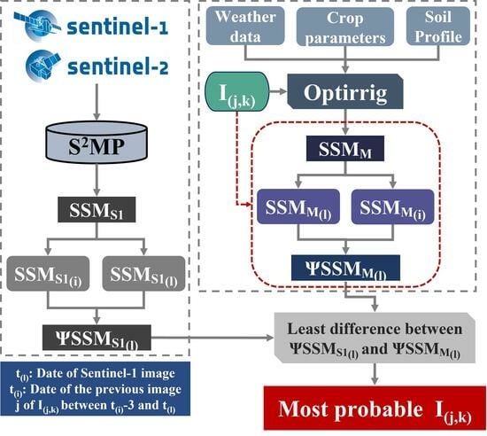
3.2.2. Inversion Approach for Irrigation Detection

The previous sections proposed two criteria (Section 3.1.2: Ψ S S M P ( l ) > Ψ S S M G ( l ) and Section 3.2.1: Ψ S S M P ( l ) > Ψ S S M r ( l ) ) to seek the possible irrigation events I(j,k) having taken place at a date j between t(i) and t(l), with an amount given by the k index. However, El Hajj et al. [72] highlighted that the SSM is estimated with an accuracy of 5 vol.%, which applies in our case to the SSM values estimated at the plot scale (µSSMp = 5%). The uncertainty on Ψ S S M P will then depend on the uncertainties in the measurements of SSMp at t(i) and t(l) as follows [94]:
μ ( l ) = Ψ S S M P l × μ S S M P l S S M P l 2 + μ S S M P i S S M P i 2
For instance, at the SAR acquisition date t(l), a value of the SSMp is recorded as S S M P ( l ) = 25 vol.%. Furthermore, our approach focuses on detecting the change in SSMP between t(l) and the previous image date t(i), where S S M P ( i ) = 15 vol.%. As a result, the ΨSSMp value is determined using Equation (2) yielding Ψ S S M P l 0.67. Subsequently, the error value on Ψ S S M P l ( μ ( l ) ) is computed using Equation (5), with a calculated value of μ ( l ) 0.26. The presence of too large uncertainties may hamper the identification of irrigation events from the previous arguments involving the Ψ S S M P ( l ) values ( Ψ S S M P ( l ) Ψ S S M G ( l ) > 0 and Ψ S S M P ( l ) Ψ S S M r ( l ) > 0 ). The following two conditions thus have to be met:
Ψ S S M P ( l ) Ψ S S M G l > μ ( l )
Ψ S S M P ( l ) Ψ S S M r l > μ ( l )
Moreover, El Hajj et al. [48] and Ouaadi et al. [44] highlighted that the effect of a rain or irrigation event on the SAR backscattering coefficient can last up to 3 days before the total dry-out of the surface. It is essential to note that the duration of dry-out largely relies on the specific soil type and its infiltration characteristics, as well as the vegetation cover. Hence, an irrigation that occurred 3 days (n = 3) before t(i) can have an effect on the change observed in SSM between S S M P I and S S M P l , and therefore, on the computed Ψ S S M P ( l ) . From this point of view, a light rain that occurred shortly before the acquisition could have the same signature as a significant rain occurring 3 days before would. This means searching for an irrigation event that occurred at the j date between t(i)−3 and t(l). As for the possible irrigation amounts, we restrained the set to realistic values with three possibilities: k = 20, 30, or 40 mm. This produced the I(j,k) combinations of dates and amounts to test, resulting in S S M R ( j , k ) values simulated by Optirrig, and therefore, in Ψ S S M R ( j , k ) values, for each I(j,k) between t(i) and t(l):
Ψ S S M R ( j , k ) = S S M R ( l ) S S M R ( i ) S S M R ( i )
The most probable irrigation combination between t(i) and t(l) was the I(j,k) that minimized the absolute value of the discrepancy between Ψ S S M R ( j , k ) and Ψ S S M P ( l ) , which was denoted |ΔΨ(j,k)|. Consequently, our goal was to find the irrigation event I(j,k) that minimized the difference between the Ψ S S M R ( j , k ) and Ψ S S M P ( l ) values. By contrast, the highest |ΔΨ(j,k)| values for a hypothesized I(j,k) event indicated the lowest probability for I(j,k) to have occurred:
| Δ Ψ ( j , k ) | = | Ψ S S M R ( j , k ) Ψ S S M P ( l ) |
When trying to minimize the |ΔΨ(j,k)| values, seeking |ΔΨ(j,k)| values as close to zero as possible, it is very likely that both negative and positive values of ΔΨ(j,k) will be encountered. A negative ΔΨ(j,k) (ΔΨ(j,k) < 0) occurs when the tested irrigation I(j,k) yields a Ψ S S M R ( j , k ) lower than Ψ S S M P ( l ) . The negative value indicates a shortfall in the impact of I(j,k) on Ψ S S M R ( j , k ) when compared with Ψ S S M P ( l ) . Conversely, a positive ΔΨ(j,k) suggests that the tested irrigation I(j,k) outperforms the Ψ S S M P ( l ) by leading to Ψ S S M R ( j , k ) values higher than Ψ S S M P ( l ) . This indicates a desire to make the ΔΨ(j,k) of an I(j,k) at j and ΔΨ(j+1,k) of an I(j,k) at j + 1 comparable and a change in sign occurs between ΔΨ(j,k) and ΔΨ(j+1,k) values, from negative to positive (10) or from positive to negative (11):
Δ Ψ ( j , k ) < 0   And   Δ Ψ ( j + 1 , k ) 0
Δ Ψ ( j , k ) > 0   And   Δ Ψ ( j + 1 , k ) 0
This change in sign is a “necessary but not sufficient condition” for the detection of an irrigation event having taken place between t(i) and t(l), as the magnitude of the change in ΔΨ(j,k) values also has to be compared with the intrinsic uncertainties, which requires
Δ Ψ ( j , k ) < μ ( l )   And   Δ Ψ ( j + 1 , k ) μ ( l )
Δ Ψ ( j , k ) > μ ( l )   And   Δ Ψ ( j + 1 , k ) μ ( l )
In the last step, Equations (12) and (13) establish the conditions for detecting an irrigation event between two specific time points, namely, t(i) and t(l). These conditions involve comparing the magnitudes of ΔΨ(j,k) values with the intrinsic uncertainties represented by μ ( l ) . Equation (12) states that if ΔΨ(j,k) is less than the negative intrinsic uncertainty ( μ ( l ) ), and ΔΨ(j+1,k) is greater than or equal to μ ( l ) , it suggests the possibility of an irrigation event that occurred between t(i) and t(l). In addition, Equation (13) implies that when the difference ΔΨ(j,k) is greater than the positive intrinsic uncertainty ( μ ( l ) ), and the subsequent difference ΔΨ(j+1,k) is less than or equal to μ ( l ) , it indicates the potential occurrence of an irrigation event between time points t(i) and t(l).
Therefore, if either condition (12) or (13) is met, the magnitudes of |ΔΨ(j,k)| and |ΔΨ(j+1,k)| are compared. The one with the smallest value represents the most probable combination of irrigation date and amount (I(j,k)). This means that if an irrigation event is detected based on either condition, the comparison of the absolute values helps to determine which I(j,k) is the most likely based on the smallest difference in ΔΨ values:
I j , k o p t = min ( Δ Ψ j , k , Δ Ψ j + 1 , k )
The minimum value of |ΔΨ(j,k)| and |ΔΨ(j+1,k)| corresponds to the irrigation event with the highest likelihood in terms of the date and amount, as it represents the irrigation combination that caused the least discrepancy in ΔΨ (between Ψ S S M R ( j , k ) and Ψ S S M P ( l ) ), considering the given uncertainties μ ( l ) .

3.3. Workflow for the Detection of Irrigation Events

Figure 5 provides a comprehensive flowchart of the proposed irrigation detection methodology, highlighting its key steps and processes. The approach aimed at retrieving the irrigation dates and amounts between a SAR acquisition date (t(l)) and the previous date (t(i)). It is good to mention that SSM values derived from S1 SAR images acquired in the ascending and descending modes were used independently. For example, over the P1 plot and at t(l) (SAR acquisition date) the detection approach was applied between the SSM derived from ascending SAR time series (MA1) at t(l) and the date of the previous image t(i) from the same time series, at a fixed interval of 6 days. For each plot and between t(l) and t(i), ten primary indicators could be derived for the plot, as presented in Table 4.
The chain started with phase 1, which consisted of distinguishing the occurrence or not of an irrigation event. It was crucial to differentiate between rainfall and irrigation events, as both can cause changes in SSM values. To eliminate the ambiguity between irrigation and rainfall events, two filters were implemented. The first filter compared the change rate of SSM at the plot scale Ψ S S M P ( l ) between t(l) and t(i) with the rate of change of SSM at the grid scale ( Ψ S S M G ( l ) ). A higher value of Ψ S S M P ( l ) indicated the presence of water application apart from rainfall.
The second filter involved a comparison between Ψ S S M P ( l ) and the simulated change rate of SSM without irrigation ( Ψ S S M r ( l ) ). Similarly, if Ψ S S M P ( l ) was higher than Ψ S S M r ( l ) , it indicated the presence of a water application other than rainfall. Once it was confirmed that an irrigation event occurred, the approach moved to phase 2, which aimed to determine the irrigation date and amount between two SAR acquisitions.
In phase 2, irrigation combinations of date j (ranging between t(i)−3 and t(l)) and dose k ( I ( j , k ) ) were entered into Optirrig between t(i) and t(l). This resulted in simulated SSM values generated by Optirrig, and corresponding change rates Ψ S S M R j , k ( l )   were computed. The objective was to find the most probable irrigation combination ( I j , k o p t ) between t(i) and t(l) by minimizing the absolute discrepancy between Ψ S S M R j , k ( l )   and Ψ S S M P ( l ) ( | Δ Ψ j , k ( l ) | ). This process is elaborated in Section 3.2.2 and illustrated in Figure 5.

3.4. Metrics Associated with Detection Issues

This section presents the results of assessing the performance of the irrigation detection approach discussed earlier by examining its capability to accurately retrieve irrigation dates and amounts over the four reference plots. Three metrics were calculated based on the concepts of true positive, false positive, and false negative, which are defined as follows. A “probably detected irrigation” I(j,k) was classified as a true positive (TP) if it was detected within three days of a real irrigation date (dRe) collected during the field trials. On the other hand, any probably detected irrigation I(j,k) that deviated significantly from these dates was classified as a false positive (FP). Conversely, if an irrigation event was not detected, it was considered a false negative (FN).
The methodology was applied to SSM temporal series from the ascending (evening overpass) and descending (morning overpass) SAR acquisitions separately due to diurnal variations caused by differences in vegetation water content between morning and evening. Studies consistently showed that the radar backscattering coefficient (σ0) is generally higher in the morning overpass compared with the evening overpass [95,96]. As a result, it is recommended to investigate each SAR temporal series separately, with one acquired in the morning and the other in the evening for each of the four reference plots (Section 2.4). In other words, the method of irrigation retrieval was employed by examining the variation in SSM between consecutive SAR images, which were denoted as t(l) and the previous image t(i), acquired within the same SAR time series acquisition. It is important to note that this approach was applied, independently, to both the ascending and descending SAR time series. Therefore, the time interval between two SSM observations was fixed at 6 days (t(l) t(i) = 6 days, revisit time of S1).
Moreover, there was an overlap in the time span between t(i) and t(l) in both ascending and descending temporal series, as the morning acquisition was only 36 h prior to the evening acquisition. For example, the evaluation of irrigation retrieval was conducted between the t(l) = 6 August 2017 SAR image acquired in the ascending mode and the date of the previous image t(i) = 31 July 2017. Similarly, in the descending mode, another SAR image was acquired at t(l) = 5 August 2017 (36 h before the evening image), with t(i) = 30 July 2017. Consequently, a real irrigation event that occurred on 3 August 2017 could potentially be detected using either the descending SAR image (t(l) = 5 August 2017) or the ascending SAR image (t(l) = 6 August 2017). As a result, two dates of irrigation detection could be recorded for the same actual irrigation date. The retrieved irrigation date that exhibited the shortest time lapse between the real irrigation event and the retrieved irrigation date was considered a true positive (TP).
The “Recall” (Re) was the first metric, representing the overall accuracy and sensitivity in detecting irrigation dates (Equation (15)). It is calculated as TP divided by TP + FN (all irrigation events). A low FN count favors a higher Re value, indicating better irrigation date detection accuracy. The “Precision” (Pn) was the second metric, defined as the ratio of TP to TP + FP (all detected events) (Equation (16)). False positive detections decrease Pn, affecting the precision. The third metric calculated the harmonic mean of recall and precision, resulting in the F-score (Equation (17)). The F-score enables comparison of the harmonic mean of Re and Pn in detecting irrigation dates across multiple cases, providing a balanced evaluation of the performance:
R e c a l l = T r u e   P o s i t i v e T r u e   P o s i t i v e + F a l s e   n e g a t i v e
P r e c i s i o n = T r u e   P o s i t i v e T r u e   P o s i t i v e + F a l s e   p o s i t i v e
F - s c o r e = 2 × R e c a l l × P r e c i s i o n R e c a l l + P r e c i s i o n
Once the probable dates of irrigation were retrieved, additional investigations were conducted to evaluate the detection of irrigation amounts applied at the detected dates of irrigation (t(m)). To assess the accuracy of the estimation, the mean absolute error percentage (MAE%) was calculated by comparing the detected irrigation amounts (AD) with the corresponding actual (real) irrigation amounts (AR) over the t(m) for the four reference plots. The MAE% quantifies the average deviation between the estimated and actual irrigation amounts, allowing for a seasonal assessment of the performance of the estimation method:
M A E % = 1 n × t ( m ) n | A D m A R m | A R ¯ × 100
where t(m) is the detected irrigation date; n is the total number of detected irrigation dates (t(m)); A R ¯ is the average of the actual irrigation amounts; and A D m and A R m are the detected and actual irrigation amounts, respectively, at t(m).
A lower MAE% indicates a higher level of accuracy in estimating the irrigation amount, as the probable amounts closely align with the actual amounts applied. Conversely, a higher MAE% suggests a larger discrepancy between the probable and actual amounts.

4. Results

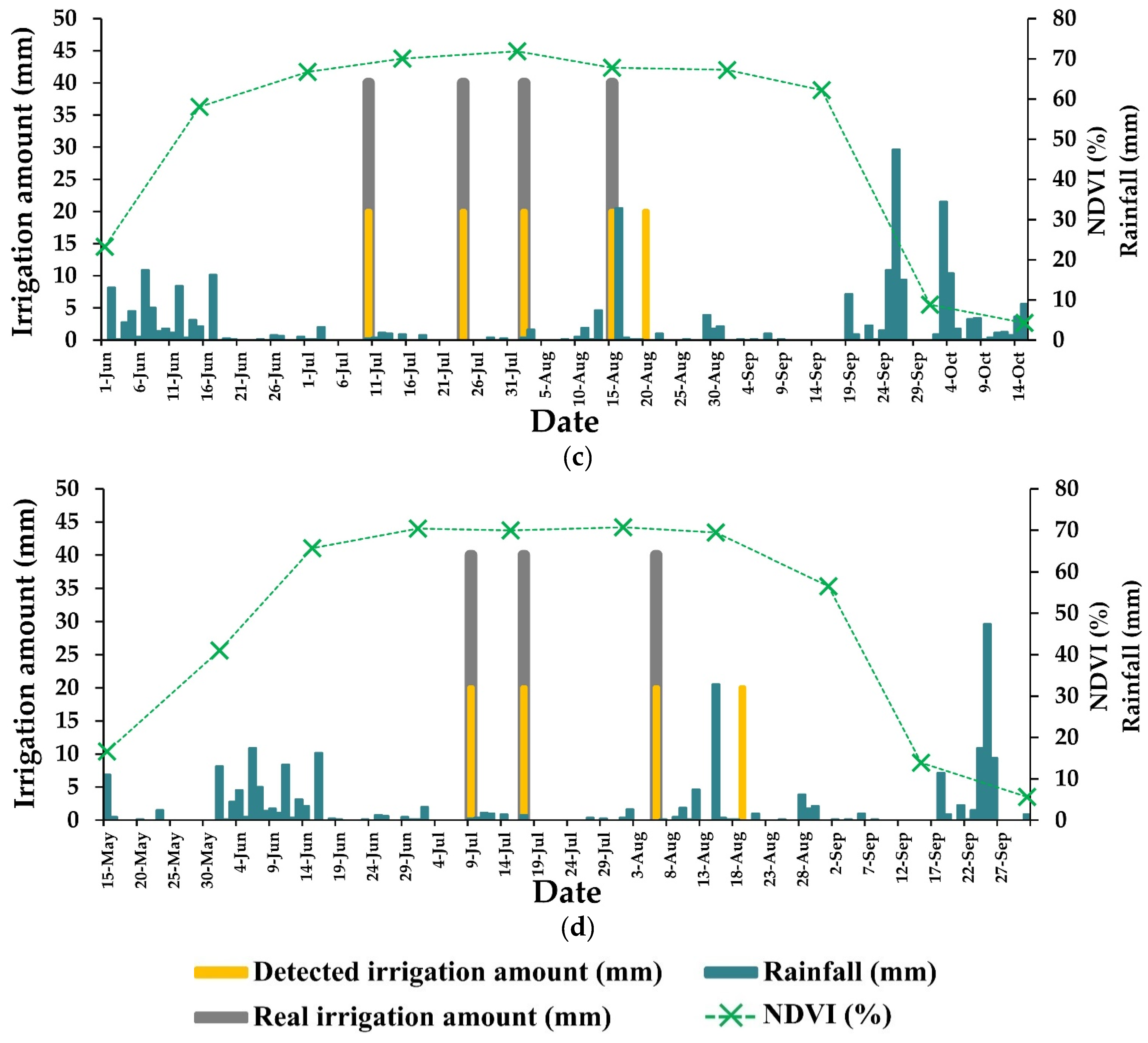
4.1. Detection of Irrigation Dates and Amounts

The proposed methodology for detecting irrigation involved two main steps. First, the SSM values derived from Sentinel-1 were analyzed at both the plot and grid scales using specific conditions, as described in Section 3.2.2, to determine whether irrigation took place between two subsequent SAR images (phase 1). If irrigation was detected, the second step involved simulating the SSM values with Optirrig, considering various combinations of irrigation dates and amounts. The goal was to find the combination that best matched the observed and simulated SSM value changes (phase 2).
Phase 1 consisted of applying two filters to distinguish between irrigation and rainfall events. The first filter compared the plot-scale SSM change rate ( Ψ S S M P ) with grid-scale change rate ( Ψ S S M G ) and the second filter compared Ψ S S M P with Ψ S S M r (rate of change of SSM simulated using Optirrig with no irrigation). Previous sections explored two irrigation detection conditions based on the difference observed between Ψ S S M P and Ψ S S M G (Equation (6)), as well as Ψ S S M r (Equation (7)). In order to identify the occurrence of an irrigation event, Ψ S S M P Ψ S S M G and Ψ S S M P Ψ S S M r have to show values higher than the error on Ψ S S M P ( μ ( l ) , Equation (5)).
Figure 6 shows an example of the detection of irrigation occurrence between the t(l) date of SAR acquisition and t(i)−3, where real irrigation was recorded (represented by blue dashed vertical lines), for the four reference plots: P1 at t(l) = 6 August 2017 (Figure 6a), P2 (Figure 6c) at t(l) = 30 June 2018, P3 at t(l) = 30 July 2019 (Figure 6e), and P4 at t(l) = 13 July 2020 (Figure 6g). The blue, green, and red horizontal dash lines represent Ψ S S M P , Ψ S S M G , and Ψ S S M r , respectively, between t(l) and t(i). To provide context, daily precipitation data (shown as blue bars) and evapotranspiration (ETo, depicted as yellow bars) obtained from nearby weather stations are included in the figures. These additional data help to understand the relationship between the Ψ S S M G and Ψ S S M r values and rainfall events. Figure 6a,c,e,g illustrate that when there was low or no precipitation, both Ψ S S M G and Ψ S S M r exhibited a slight decrease or remained stable. Concurrently, in all four cases documented, Ψ S S M P demonstrated higher values than both Ψ S S M G and Ψ S S M r . This observed difference, which exceeded the error margin of Ψ S S M P ( μ ( l ) ), confirming the conditions in Equations (6) and (7) were met, which served as evidence of irrigation occurrence in the four examples.
In phase 2, when an irrigation occurrence was identified between t(i) and t(l), further investigations were conducted to determine the probable date and amount of irrigation. This involved simulating the Ψ S S M R ( j , k ) (black lines) for each irrigation combination (I(j,k)), where the date j ranged from t(i)−3 to t(l), and the tested amount k was set to 20, 30, and 40 mm. The purpose of these simulations was to compare the Ψ S S M R ( j , k ) values with the Ψ S S M P and minimize the difference between them ( | Δ Ψ ( j , k ) | = | Ψ S S M R ( j , k ) Ψ S S M P | , Equation (9)) in order to derive insights about the most likely I(j,k). The evolution of Δ Ψ ( j , k ) for different I(j,k) values of date j and dose k is presented in Figure 6b,d,f,h for each of the examples where irrigation occurrence was suspected in phase 1 (Figure 6a,c,e,g).
For instance, an occurrence of irrigation was identified between t(i) = 31 July 2017 and t(l) = 6 August 2017, with ascending SAR image dates (Figure 6a). A detailed analysis was carried out in Figure 6b to determine the specific irrigation date and amount that probably occurred between t(i)−3 and t(l). This investigation involved examining the changes in Δ Ψ ( j , k ) for different irrigation dates j ranging from 28 July 2017 to 5 August 2017, and k amounts of 20, 30, and 40 mm to compare Δ Ψ ( j , k ) values to the error on Ψ S S M P ( μ ( l ) ). It is important to note that the error on Ψ S S M P between t(i) and t(l) was μ ( l ) = 0.068.
Concerning the plot P1 (Figure 6a,b), on the date j = 31 July 2017, the observed values of Δ Ψ ( j , k ) ranged from −0.71 for k = 20 mm to −0.76 for k = 30 and 40 mm, all of which were lower than − μ ( l ) . This discrepancy could be attributed to significantly lower Ψ S S M R ( j , k ) values compared with Ψ S S M P ( Δ Ψ ( j , k ) < μ ( l ) ) observed at j in Figure 6a. Furthermore, on j + 1 = 1 August 2017, the Δ Ψ ( j + 1 , k ) values exhibited positive values greater than μ ( l ) ( Δ Ψ ( j + 1 , k ) = 0.22 > μ ( l ) ) for k = 20, 30, and 40 mm. This satisfied one of the criteria for identifying the most likely irrigation event (I(j,k)), as stated in Equation (12) ( Δ Ψ ( j , k ) < μ ( l ) and Δ Ψ ( j + 1 , k ) μ ( l ) ).
Therefore, it can be concluded that an irrigation event occurred between j = 31 July 2018 and j + 1 = 1 August 2017. To determine the most probable irrigation date ( I j , k o p t ) the irrigation combination (I(j,k)) leading to the smallest absolute value between Δ Ψ ( j , k ) and Δ Ψ ( j + 1 , k ) was identified, as described in Equation (14) ( I j , k o p t = min ( Δ Ψ j , k , Δ Ψ j + 1 , k ) ). Accordingly, since | Δ Ψ ( j + 1 , k ) | = 0.22 (regardless of the amount k) is smaller than | Δ Ψ ( j , k ) | = 0.71 for k = 20 mm and | Δ Ψ ( j , k ) | = 0.76 for k = 30 and 40 mm, the irrigation date j + 1 = 1 August 2017 was identified as the most probable date of I j , k o p t . However, the analysis of Δ Ψ ( j + 1 , k ) did not reveal any discernible variations across different irrigation amounts k = 20, 30, and 40 mm, making it impossible to identify irrigation amounts beyond k = 20 mm.
In Figure 6b, the actual irrigation date, marked in blue, was 3 August 2017. Therefore, the detected irrigation date (1 August 2017) had a time difference of 2 days compared with the actual date.
Based on the reasoning above, for the remaining three cases over P2 (Figure 6c,d), P3 (Figure 6e,f), and P4 (Figure 6g,h), the actual irrigation dates were successfully detected with a time lapse of 1 day from the actual irrigation dates:
  • For P2: The detected irrigation date was 26 June 2018 and the actual date was 27 June 2018;
  • For P3: The detected irrigation date was 25 July 2019 and the actual date was 24 July 2019;
  • For P4: The detected irrigation date was 08 July 2020 and the actual date was 09 July 2020.
Furthermore, it is noteworthy that the detected irrigation amounts for the P2, P3, and P4 plots were consistently k = 20 mm. This demonstrates that the analysis did not identify any discernible differences in the Δ Ψ ( j , k ) values when testing irrigations with different amounts (k = 20, 30, and 40 mm) at the detected irrigation dates.

4.2. Irrigation Events Detection Performance

The performance of the irrigation dates detection was evaluated using the accuracy metrics (recall, precision, and F-score) across the four reference plots. The irrigation detection approach yielded varying levels of accuracy across different plots (Figure 7).
In P1 in Montpellier, 70% of the irrigation dates were correctly identified (recall), with 88% accuracy among the detected dates (precision). The F-score, which is a combined measure of precision and recall, achieved a satisfactory value of 78%, indicating a reasonably balanced performance in identifying irrigated areas. In P2, the recall was slightly higher at 75%, indicating that 25% of the irrigated areas were not correctly detected. However, the precision was 100%, meaning that all the identified irrigated events were accurate. The associated F-score was 86%, indicating a good overall performance with a trade-off between recall and precision. For P3 and P4, both exhibited a high recall of 100%, indicating that all irrigated events were correctly identified. However, the precision varied between 80% for P3 and 75% for P4, suggesting that 20% to 25% of the detected irrigated areas were false positives. The F-scores were 89% for P3 and 86% for P4, demonstrating a good overall performance with a slightly higher emphasis on recall. These results highlight the strengths of the approach, providing valuable insights for improving the accuracy and reliability of irrigation date detection. The accuracy of the irrigation dates detection was impacted by the presence of false detections, primarily attributed to the low accuracy of SSM estimation under dense vegetation covers and/or the SAR revisit time (see the Discussion section).
To ensure operational effectiveness, it is important to not only identify irrigation dates but also estimate the irrigation amounts. Therefore, we conducted a comparison between the detected amounts (AD) and the actual amounts (AR) on the P1, P2, P3, and P4 plots over the irrigation dates detected using the SSM derived from SAR temporal series in the ascending and descending modes. In Figure 8, both the detected dates and irrigation amounts were presented alongside the real field data. The figure illustrates all observed Sentinel-2 NDVI values, categorizing them based on the vegetative or reproductive stages. It also highlights instances of missed irrigation detection, false detections, and correct detections. Within Figure 8, grey and yellow bars correspond to the real and detected irrigation amounts, respectively. Thus, a true irrigation date detection is represented when a yellow bar is positioned over a grey bar for each actual irrigation date. Conversely, a false irrigation detection (false positive) is indicated by a single yellow bar, indicating that our approach detected irrigation on a date that did not correspond with an actual irrigation event. Likewise, an undetected irrigation date (false negative) is represented by a single grey bar, indicating that our approach failed to detect an irrigation date.
In the present study, Figure 8 displays only three instances of false positive date detections, specifically in Figure 8a on the date 01 July (DOY = 182), in Figure 8c on the date 20 August (DOY = 233), and in Figure 8d on the date 19 August (DOY = 232). Moreover, the analysis revealed the failure to detect four irrigation events. Among these undetected events, three occurred in Figure 8a on the dates 11 August, 22 August, and 26 September (DOYs = 223, 234, 269), while the fourth one took place in Figure 8b on the date 5 August (DOY = 217).
These results illustrate one of the inherent limitations of the approach employed, which relies on the progressive growth of crop cover, as indicated by the ascending dynamics of NDVI, along with the revisit time of the SAR data. This limitation explains the occurrence of false detections during the reproductive stage and the missed detections of actual irrigation events. The reliance on crop cover development and the timing of SAR observations introduced constraints on the accuracy of the detection method (see the Discussion section).
Next, the investigation focused on analyzing the changes in ΔΨ(j,k) over the detected irrigation dates (t(m)) to gain insights into the applied amounts of irrigation water. Among the detected irrigation dates, a dose of k = 20 mm was identified as the most probable amount of irrigation for five occurrences and k = 30 mm for two occurrences out of a total of seven detected irrigation dates out of the 10 actual irrigation dates. In the case of plots P2, P3, and P4, a dose of k = 20 mm was detected for all the detected irrigation dates. However, the detected irrigation amounts underestimated the real irrigation amounts in most cases.
Therefore, it could be valuable to conduct a seasonal assessment of the irrigation amounts to provide insights into the performance of the amount-detection method throughout the season. The MAE% (Equation (18)) served as a measure of the average deviation between the detected irrigation amounts (AD) with the corresponding actual (real) irrigation amounts (AR) for all the detected irrigation dates (t(m)) in the four reference plots. A lower MAE% indicates a higher level of accuracy in estimating the irrigation amounts, indicating a close alignment between the estimated and actual amounts applied. Conversely, a higher MAE% suggests a larger discrepancy between the estimated and actual amounts. Based on the obtained results, a MAE% of 16.4% was achieved for the P1 plot in Montpellier, indicating relatively high accuracy in estimating the irrigation amounts. The estimated amounts closely matched the actual amounts applied in this plot. However, for the Tarbes plots (P2, P3, and P4), a MAE% of 50% was obtained, indicating a larger discrepancy between the estimated and actual amounts. The estimation method exhibited a lower level of accuracy in these plots, with more significant deviations between the estimated and actual amounts applied.

5. Discussion

The methodology aimed to determine irrigation dates and amounts at the plot level by integrating surface soil moisture (SSM) data obtained from Sentinel-1 (SSMS1) into Optirrig using an inversion technique. To achieve this, we compared the change in SSMS1 between two Sentinel-1 SAR acquisition dates, namely, t(l) and the previous date t(i), with the change in SSM simulated by Optirrig under various combinations of irrigation dates and amounts (I(j,k), where j represents the date and k represents the amount) injected into the model.
The analysis that produced the results presented in the previous sections focused on determining irrigation dates and amounts for which the disparity between the change in SSM predictions and simulations between two SAR observations (i) was minimized, aiming for a value as close to zero as possible, and (ii) met specific criteria by demonstrating significant changes between the SSM simulated for different irrigation scenarios in Optirrig and its difference with the SSM obtained from Sentinel-1 data. These criteria were applied using a change detection approach commonly used in signal analysis and remote sensing applications. For a more detailed understanding of the process of inversion and the specific selection criteria utilized to detect irrigation events, please refer to Figure 6 and its accompanying explanations.
The method yielded significant results, highlighting the value and interest in combining SSM derived from Sentinel-1 SAR data and Optirrig SSM simulations. This combination demonstrated the potential benefits of detecting irrigation events over maize plots. However, there were limitations to detecting irrigation events through the combined use of SSMS1 and Optirrig SSM simulations, which could result in both missed (false negative) and false positive irrigation detections, between two SAR observations. These limitations primarily stemmed from four factors: (1) the 6-day temporal resolution of the Sentinel-1 SAR being insufficient to detect all the irrigation events, (2) heavy rainfall and soil saturation, (3) the limit of penetration of the C-band SAR signal in dense vegetation cover, and (4) farmer’s irrigation practices.

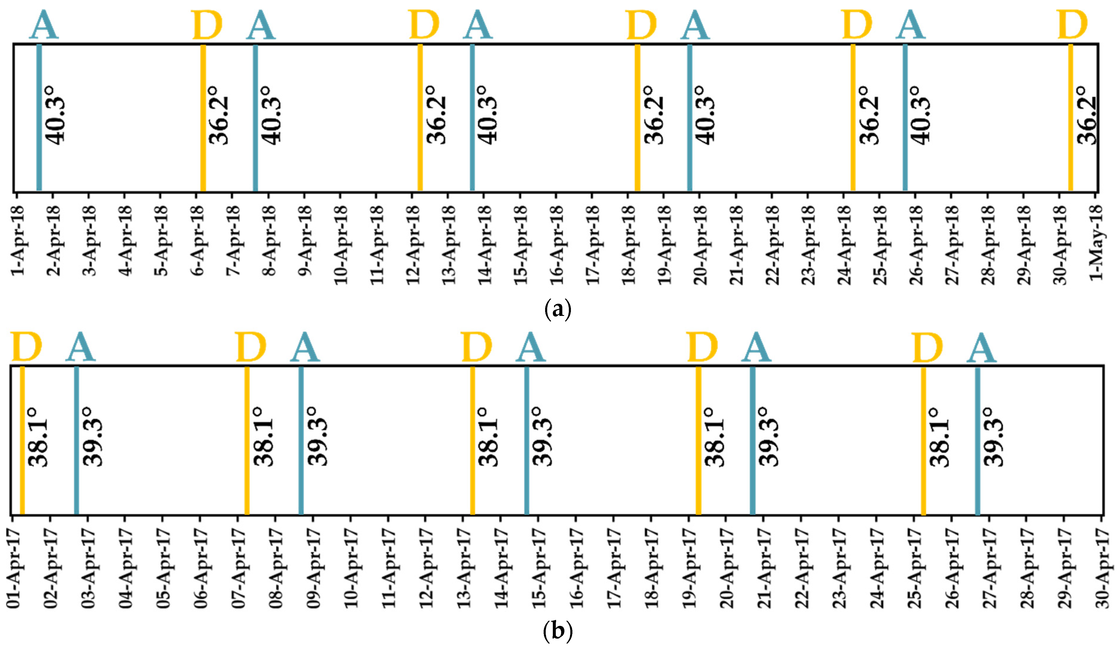
5.1. Sentinel-1 Revisit Time

First, these limitations were influenced by the soil texture, field capacity, and rapid drying of the soil, which could impact the effectiveness of irrigation event detection. The rapid drying of the soil necessitated a sensor with a higher temporal resolution to detect quick changes in soil moisture content, such as an increase due to irrigation followed by a decrease due to drying. Previous studies confirmed the importance of a maximum time delay of three days between an irrigation event and the subsequent SAR image to accurately detect the event’s impact on the SAR backscattering signal [44,48]. Beyond this timeframe, it becomes challenging to detect the effect of an irrigation event. The temporal resolution of the S1 SAR should ideally be no more than three days for a more effective irrigation detection [16,43].
The 6-day revisit time of the S1 SAR constellation poses a significant challenge in detecting irrigation events due to the rapid dry-out of certain soil surfaces, as previously mentioned. It also creates difficulties in distinguishing the effects of rainfall and irrigation events, especially in the worst-case scenario, where both rain and irrigation occur between the same two consecutive acquisition dates. The increase in SSM values after rainfall and irrigation may be similar, even for different amounts, which makes it even more difficult. In the specific case described in the P2 plot (Figure 8b), there was a missed irrigation detection on 5 August 2018 following a heavy rainfall event ( 33 mm) on 2 August 2018, which likely caused a significant increase in soil moisture, resulting in high SSM values. This missed detection could be attributed to the method’s inability to effectively distinguish between the impact of the heavy rainfall and the irrigation. As a result, the occurrence of the irrigation event went undetected, leading to a false negative detection. It is worth noting that this particular case was observed only once in the analysis due to the applied filters and methods used to distinguish between rainfall and irrigation events. These filters involved analyzing Optirrig SSM simulations and SSM at both plot and grid scales, as described in Section 3. Unfortunately, due to an anomaly affecting S1B, the revisit time for S1 SAR data has increased from 6 days to 12 days, as only S1A remains operational. This reduced revisit frequency presents a challenge for SSM estimation frequency and accurate irrigation detection and monitoring. To address this challenge, an effective strategy involves integrating SSM estimations from other SAR data sources. Collaborating with SAR satellites like ALOS PALSAR, RADARSAT, and COSMO-SkyMed can provide supplementary SSM data, effectively augmenting the frequency of observations. Additionally, leveraging the benefits of small- or micro-SAR satellites, which can be launched in constellations, offers a promising solution. These satellites provide increased revisit frequencies and higher spatial resolutions, which are essential for capturing frequent and detailed observations of irrigation patterns and soil moisture dynamics. By combining the data from different SAR sources, both large and small, a more comprehensive dataset covering a broader range of time intervals and spatial scales can be created. This integrated approach can significantly enhance the potential for the precise analysis of irrigation patterns and soil moisture dynamics, despite the limitations imposed by the reduced revisit time. Moreover, there is promising news on the horizon—the launch of a new constellation of SAR satellites, namely, Sentinel-1C, is planned for the end of 2023. Once operational, Sentinel-1C is expected to mitigate the revisit time challenge by providing more frequent observations, bolstering the accuracy of irrigation detection and soil moisture estimation efforts.

5.2. Climatic and Soil Conditions

Optirrig SSM simulations were crucial in differentiating rainfall and irrigation events. In the present study, the observed SSM changes derived from the S1 data at the plot and grid scales were compared with the simulated SSM changes from Optirrig under rainfall conditions. This comparison provided valuable insights into the expected SSM values, allowing for the accurate interpretation of S1 data and avoiding irrigation misinterpretations. However, Optirrig filter effectiveness may vary depending on specific cases, and the context and limitations should be considered.
Indeed, heavy rainfall can also lead to false positive irrigation detection, particularly in situations where there is a moderately developed maize cover that restricts soil evaporation [97]. This effect is particularly pronounced during the early vegetative stage and late reproductive stages of maize growth when the vegetation cover is not dense enough to attenuate the SAR signal (NDVI < 0.7) [49], and thus, allow for effective monitoring of the underlying SSM. During this period, the moderately dense vegetation canopy acts as a barrier, limiting the evaporation of soil moisture. In this context, if a heavy rainfall event occurs, the soil can become saturated with water, which means that the soil has reached its maximum water-holding capacity and cannot absorb any more moisture. As a result, the soil remains wet even after the rainfall has ceased. When using Optirrig SSM simulations, which estimate SSM levels based on rainfall inputs, simulations may not exhibit significant changes between two consecutive SAR acquisition dates when soil saturation occurs. This is because the simulations account for the limited capacity of the soil to absorb additional moisture beyond saturation. In fact, the detection of irrigation amounts was found to be less efficient for the plots in the humid climate of Tarbes (P2, P3, and P4) compared with the “semi-arid” climate of Montpellier (P1). For the P1 plot, the estimation of the seasonal irrigation amounts exhibited a relatively high accuracy, with a mean absolute error percentage (MAE%) of 16.4%. In contrast, for the P2, P3, and P4 plots in the humid climate, a higher MAE% of 50% was obtained, suggesting a larger discrepancy between the detected and actual amounts of irrigation. This discrepancy was likely due to the challenges posed by the humid climate, where heavy rainfall events can contribute to soil saturation, thereby affecting the accuracy of irrigation detection and amount estimation. The effectiveness of the irrigation detection approach, particularly in estimating irrigation amounts, appears to be influenced by the local climate conditions, with the humid climate introducing additional complexities. Moreover, SSMS1 values at the plot scale may remain high due to the water content in the saturated soil, where evaporation and rapid dry-out are restrained. In fact, the S1 SAR signal is sensitive to the presence of water in the soil, resulting in elevated SSM values. However, at the grid scale (10 km × 10 km), SSM values calculated over bare soils may show stability or decrease since bare soil areas have higher evaporative capacities compared with plots with developed maize cover. In such situations, the method used for irrigation detection may interpret the observed increase in SSM variation at the plot scale as an indication of irrigation occurrence. In other words, Optirrig simulations for rain-fed conditions may not show substantial SSM changes, and the S1 SSM values at the plot scale may remain high, leading to false irrigation detection. In the study, three false positive irrigation detections were observed after relatively heavy rainfall events, specifically over P1 on 01-Jul (DOY = 182), P3 on 20 August (DOY = 232), and P4 on 19 August (DOY = 232). These false positive detections occurred due to the restrained evaporation of soil moisture under developed maize cover (NDVI values that ranged from 0.6 to 0.7), which resulted in high SSM values that were mistaken as indications of irrigation occurrence.

5.3. C-Band SAR Signal Penetration through Dense Vegetation Cover

The limited penetration of the C-band SAR signal through dense vegetation cover has a direct impact on the effectiveness of irrigation detection using Sentinel-1 SAR data. The method proposed in this study relies on analyzing the change of SSM derived from S1 data and SSM simulations through Optirrig to identify irrigation events. However, when the SAR signal is impeded by dense vegetation, the accurate estimation of SSM becomes challenging. This limitation arises from the S1 signal’s inability to penetrate through vegetation and reach the surface soil. Research conducted by El Hajj et al. [49] focused on the penetration of the C-band SAR signal across different plots of maize, wheat, and grassland. Their findings revealed that the C-band SAR signal’s penetration is limited to an NDVI value of 0.7. Therefore, dense vegetation cover can hinder the detection of irrigation events due to the SAR signal’s limited sensitivity to surface soil moisture. Therefore, if the C-band SAR signal is unable to penetrate dense vegetation, the estimated SSM values may not adequately represent the irrigation-induced changes in soil moisture. Consequently, the threshold criteria, which were based on S1 and Optirrig SSM simulations, used in this method to identify irrigation events (Section 3.2.2) may not be met, resulting in missed detections or false negative results. In our case, missed detections were observed for peak NDVI values between 0.7 and 0.8 over the P1 and P2 plots (Figure 8a,b). These findings are consistent with the results obtained by El Hajj et al. [48] for grassland plots and Le Page et al. [43] for maize plots. Both studies highlight the limitations of irrigation detection over dense vegetation cover (NDVI > 0.7) due to the restricted penetration of the C-band SAR signal.

5.4. Farmer’s Irrigation Practice Variability

One additional reason for missed or false negative detections of irrigation events is the variation in farmers’ irrigation practices, particularly in terms of timing and quantity. It is likely that the accurate detection of irrigation is hindered because farmers do not always follow the irrigation decisions based on a soil water balance and exact crop water requirements or decisions that could be advised by Optirrig, including triggers, criteria, and doses. Instead, their irrigation decisions are influenced by a combination of factors, including their experience, local knowledge, and perceptions of water availability. They may prioritize ensuring an adequate water supply to the crops, leading to irrigation amounts that exceed the exact crop water requirements. For instance, it appeared to be challenging to detect the last irrigation applied on 26-Sep (DOY = 269) over the P1 plot. This irrigation event may not be deemed necessary from the water balance perspective of Optirrig, but farmers still apply it for reasons such as grain filling or to prevent soil crusting [98]. On the other hand, Optirrig relies on a soil water balance equation to simulate and predict the soil moisture content in the root zone of the crops. This equation takes into account factors such as precipitation, evapotranspiration, soil characteristics, and irrigation events to estimate the water balance in the soil. Therefore, when testing different irrigation dates and amounts, Optirrig determines the exact SSM induced by the irrigation and other water sources (rainfall), which may not align precisely with farmers’ irrigation timing and the amounts they apply. In the present study, we consistently noticed that the detected irrigation amounts in the four plots (P1, P2, P3, and P4) were consistently lower than the actual irrigation amounts applied by the farmers in the field. This indicates a case of underestimation or missed detection of irrigation events. This discrepancy between farmers’ actual irrigation practices and the detected irrigation amounts can explain the low accuracy of detecting real irrigation amounts (which is somehow expected as Optirrig is used here as a tool for analysis, not for recommendations). Farmers tend to overestimate crop water requirements and apply higher levels of irrigation that do not match the exact crop water needs.

5.5. Uncertainties Associated with Optirrig’s Simulations

In a broader context, the SSM simulations in Optirrig are subject to inherent uncertainties, which can impact the accuracy of irrigation detection. These uncertainties arise from several factors, including the variability in input parameters and the temporal dynamics of vegetation [99,100]. In fact, the accuracy of SSM simulations depends on the availability and quality of input parameters, such as soil properties, vegetation characteristics, and meteorological data [101]. However, these parameters can vary spatially and temporally, leading to uncertainties in the simulations [102]. Moreover, the temporal dynamics of vegetation, including growth stages, leaf area index, and canopy density, can also introduce uncertainties in SSM simulations. Vegetation plays a crucial role in the water balance of the soil–plant–atmosphere system, as it affects evapotranspiration rates and soil moisture depletion in crop models [103], such as Optirrig. However, accurately representing the dynamics of vegetation within the model is challenging. Changes in vegetation characteristics over time can lead to variations in evapotranspiration rates and water uptake by plants, impacting the simulated SSM values [104] and potentially affecting the detection of irrigation events. To mitigate these uncertainties, there is growing interest in incorporating multiple external and independent data, such as radar and optical data, in various irrigation mapping, detection, and crop monitoring approaches [105,106]. In a recent study, Nie et al. [107] demonstrated the potential of using remotely sensed vegetation and soil moisture observations (MODIS LAI and SMAP data) to constrain irrigation estimation in the Noah-MP land surface model. Results have shown that incorporating these constraints reduces model sensitivity to irrigation parameterization, improves characterization of irrigation patterns and their effects on evapotranspiration and soil moisture, and corrects for vegetation conditions and irrigation timing. This approach highlights the importance of utilizing remotely sensed data for irrigation detection and provides a less engineered method to constrain irrigation modeling uncertainty. The integration of several remote sensing data sources aims to inform crop models and reduce uncertainties associated with irrigation estimation. In the present case, incorporating both radar data for soil surface moisture estimates and optical data, such as LAI observations, into the inversion process would likely yield substantial benefits. By combining these data, it becomes possible to constrain both the water balance and crop growth schemes of Optirrig. This approach enhances the accuracy and reliability of the crop model, enabling improved detection of irrigation events and more precise estimation of crop water requirements. For instance, Ferrant et al. [106] developed and tested a methodology using Sentinel-1 and Sentinel-2 satellite observations to monitor the spatiotemporal variations in irrigated areas in the Kudaliar catchment, Telangana State, South India. The methodology employed a machine learning algorithm and achieved high accuracy by combining radar and optical data. The results showed the variability of irrigated areas across different seasons and highlighted the potential of this approach for near-real-time monitoring in South India. These findings contribute to calibrating agro-hydrological models and assessing the impact of agriculture on water resources. Incorporating biophysical data, such as LAI, from high-resolution optical images, like those from Sentinel-2, in conjunction with SSM SAR estimations can greatly benefit the constraint of Optirrig simulations. This combination of data sources enhances the monitoring of irrigation practices by providing complementary information on vegetation dynamics and soil moisture levels. By integrating LAI and SSM data, Optirrig can achieve improved accuracy and reliability in detecting and monitoring irrigation practices. The results of the present study demonstrate the effectiveness of our approach and offer valuable insights into the precision and dependability of irrigation date and amount detections, providing reliable information for monitoring irrigation practices. With further validation using a larger dataset encompassing diverse crops and irrigation methods, we could potentially develop a near-real-time tool for irrigation detection.

6. Conclusions

This study aimed at the detection of irrigation dates and amounts at the plot level by integrating Sentinel-1 surface soil moisture (SSMS1) data into Optirrig using an inversion technique, which fits in the idea of providing methods for the supervision of irrigated perimeters. The methodology involved comparing the change in SSMS1 between two SAR acquisition dates with the change in SSM simulated by Optirrig for various combinations of irrigation dates and amounts. Two filters were applied to remove the ambiguity between irrigation events and rainfall, and thus, determine the occurrence or not of a potential irrigation event. These filters relied on comparing the change in the SSM at plot scale to the change in SSM at grid scale (10 km × 10 km) and in the SSM simulated by Optirrig under the effect of the rainfall alone. The detected irrigation date with the shortest time difference from the real irrigation event date was considered the detected event. To assess the accuracy and robustness, the method was tested against documented situations in four experimental maize plots located in the Occitanie Region of southern France (near Montpellier and Tarbes). This testing helped to evaluate the method’s applicability for operational purposes, such as supervising irrigated territories, and provided insights into its strengths, limitations, and potential improvements.
The performance of the inversion process in retrieving correct irrigation dates between two successive Sentinel-1 images was evaluated using three metrics: recall, precision, and F-score. These metrics assess the accuracy based on false negative (missed irrigation detection), false positive (incorrectly detected irrigation), and true positive detections. The evaluation of the inversion process using real irrigation data yielded promising results. The recall, which represents the ratio of true positive detections to the sum of the true positives and false negatives, was determined to be 86.2%. This indicates that the inversion process successfully captured a significant portion of the irrigation events. Similarly, the precision, which denotes the ratio of true positive detections to the sum of the true positives and false positives, was calculated to be 85.7%. This metric demonstrates the accuracy of the inversion process in correctly identifying irrigation events while minimizing false detections. Furthermore, the assessment of seasonal irrigation amounts estimation performance for each plot revealed variations based on the climate conditions. The efficiency of irrigation amount detection proved to be lower for the plots situated in the humid climate of Tarbes in comparison with the “semi-arid” climate of Montpellier. The estimation of seasonal irrigation quantities for the P1 plot demonstrated relatively accurate results. However, for the plots in Tarbes, a notably higher mean absolute error percentage (MAE%) was recorded, indicating a more significant disparity between the detected and actual irrigation amounts.
A comprehensive and meticulous analysis of the results provided valuable insights into the weaknesses and instances of failure in detecting irrigation dates and amounts. The examination of missed and false irrigation detection brought to light the primary limitations of the method, which could be attributed to two key factors. First, the characteristics of the Sentinel-1 constellation, including its 6-day revisit time and the challenges associated with signal penetration in dense maize cover, were identified as contributing to the limitations. Additionally, it was found that the parameterization of Optirrig for SSM simulations did not precisely align with the irrigation practices and decision rules followed by farmers, further impacting the accuracy of the method.
The incorporation of external information and constraints to enhance the inversion process represents a valuable perspective for future practical implementations of the method, both at specific plots and across larger irrigated areas. One promising approach is the incorporation of additional data sources and constraints to inform and refine the inversion process in Optirrig. For instance, combining soil surface moisture estimates obtained from radar data with leaf area index (LAI) observations derived from optical data can offer significant benefits to the inversion process. Especially notable is the upcoming launch of the new SAR mission NISAR in the L-band, which offers the potential for more precise and deeper SSM (surface soil moisture) estimations. This capability will be particularly advantageous in regions with dense canopy cover, as the L-band SAR signal can penetrate further into the soil and crop canopy. L-band SAR data bring a distinct advantage due to their superior ability to penetrate dense vegetation cover, resulting in more accurate estimations of soil moisture content within such areas. To tackle the challenge of observation frequency and to further refine the accuracy of soil moisture estimations and irrigation detection, a potential strategy involves incorporating L-band NISAR data as an additional data source complementing the existing C-band data. The integration of these two data types can lead to an increased observation frequency, thereby furnishing valuable insights into both water balance and crop growth dynamics within the Optirrig model. By leveraging such complementary information and further validation using a larger dataset encompassing diverse crops and irrigation methods, it becomes possible to enhance the accuracy and reliability of the method’s performance and potentially develop a near real-time tool for irrigation detection.

Author Contributions

Conceptualization, M.H., B.C. and N.B.; data curation, M.H., B.C. and D.C.; formal analysis, M.H., B.C. and N.B.; methodology, M.H., B.C. and N.B.; software, M.H., B.C. and N.B.; supervision, N.B. and B.C.; validation, M.H., B.C., N.B. and M.Z.; writing—original draft, M.H.; writing—review and editing, B.C., N.B., D.C. and M.Z. All authors have read and agreed to the published version of the manuscript.

Funding

This research received funding the National Research Institute for Agriculture, Food and the Environment (INRAE); and the RSEAU project financed by the French Environment and Energy Management Agency (ADEME).

Data Availability Statement

The data presented in this study are available on request from the corresponding author.

Acknowledgments

The authors wish to thank the French Space Study Center (CNES, TOSCA 2021) and the National Research Institute for Agriculture, Food and Environment (INRAE). The authors wish to acknowledge the support and funding received from Campus France and CNRS-L for M. Hamze’s PhD thesis. Furthermore, they extend their appreciation to the European Space Agency (ESA) for granting access to the Sentinel-1 data and to the French Land Data Center (Theia) for providing the Sentinel-2 data with atmospheric corrections.

Conflicts of Interest

The authors declare no conflict of interest.

References

  1. Wu, B.; Tian, F.; Zhang, M.; Piao, S.; Zeng, H.; Zhu, W.; Liu, J.; Elnashar, A.; Lu, Y. Quantifying Global Agricultural Water Appropriation with Data Derived from Earth Observations. J. Clean. Prod. 2022, 358, 131891. [Google Scholar] [CrossRef]
  2. Harmanny, K.S.; Malek, Ž. Adaptations in Irrigated Agriculture in the Mediterranean Region: An Overview and Spatial Analysis of Implemented Strategies. Reg. Environ. Chang. 2019, 19, 1401–1416. [Google Scholar] [CrossRef]
  3. Raza, A.; Razzaq, A.; Mehmood, S.S.; Zou, X.; Zhang, X.; Lv, Y.; Xu, J. Impact of Climate Change on Crops Adaptation and Strategies to Tackle Its Outcome: A Review. Plants 2019, 8, 34. [Google Scholar] [CrossRef]
  4. Fahad, S.; Bajwa, A.A.; Nazir, U.; Anjum, S.A.; Farooq, A.; Zohaib, A.; Sadia, S.; Nasim, W.; Adkins, S.; Saud, S.; et al. Crop Production under Drought and Heat Stress: Plant Responses and Management Options. Front. Plant Sci. 2017, 8, 1147. [Google Scholar] [CrossRef]
  5. Piscitelli, L.; Colovic, M.; Aly, A.; Hamze, M.; Todorovic, M.; Cantore, V.; Albrizio, R. Adaptive Agricultural Strategies for Facing Water Deficit in Sweet Maize Production: A Case Study of a Semi-Arid Mediterranean Region. Water 2021, 13, 3285. [Google Scholar] [CrossRef]
  6. Elwan, E.; Page, M.L.; Jarlan, L.; Baghdadi, N.; Brocca, L.; Modanesi, S.; Dari, J.; Segui, P.Q.; Zribi, M. Irrigation Mapping on Two Contrasted Climatic Contexts Using Sentinel-1 and Sentinel-2 Data. Water 2022, 14, 804. [Google Scholar] [CrossRef]
  7. Saux-Picart, S.; Ottlé, C.; Decharme, B.; André, C.; Zribi, M.; Perrier, A.; Coudert, B.; Boulain, N.; Cappelaere, B.; Descroix, L.; et al. Water and Energy Budgets Simulation over the AMMA-Niger Super-Site Spatially Constrained with Remote Sensing Data. J. Hydrol. 2009, 375, 287–295. [Google Scholar] [CrossRef]
  8. Singh, M.; Karada, M.S.; Rai, R.K.; Pratap, D.; Agnihotri, D.; Singh, A.K.; Singh, B.K. A Review on Remote Sensing as a Tool for Irrigation Monitoring and Management. Int. J. Environ. Clim. Chang. 2023, 13, 203–211. [Google Scholar] [CrossRef]
  9. Babaeian, E.; Sidike, P.; Newcomb, M.S.; Maimaitijiang, M.; White, S.A.; Demieville, J.; Ward, R.W.; Sadeghi, M.; LeBauer, D.S.; Jones, S.B.; et al. A New Optical Remote Sensing Technique for High-Resolution Mapping of Soil Moisture. Front. Big Data 2019, 2, 37. [Google Scholar] [CrossRef] [PubMed]
  10. Longo-Minnolo, G.; Consoli, S.; Vanella, D.; Ramírez-Cuesta, J.M.; Greimeister-Pfeil, I.; Neuwirth, M.; Vuolo, F. A Stand-Alone Remote Sensing Approach Based on the Use of the Optical Trapezoid Model for Detecting the Irrigated Areas. Agric. Water Manag. 2022, 274, 107975. [Google Scholar] [CrossRef]
  11. Demarez, V.; Helen, F.; Marais-Sicre, C.; Baup, F. In-Season Mapping of Irrigated Crops Using Landsat 8 and Sentinel-1 Time Series. Remote Sens. 2019, 11, 118. [Google Scholar] [CrossRef]
  12. Ambika, A.K.; Wardlow, B.; Mishra, V. Remotely Sensed High Resolution Irrigated Area Mapping in India for 2000 to 2015. Sci. Data 2016, 3, 160118. [Google Scholar] [CrossRef] [PubMed]
  13. Dari, J.; Brocca, L.; Quintana-Seguí, P.; Escorihuela, M.J.; Stefan, V.; Morbidelli, R. Exploiting High-Resolution Remote Sensing Soil Moisture to Estimate Irrigation Water Amounts over a Mediterranean Region. Remote Sens. 2020, 12, 2593. [Google Scholar] [CrossRef]
  14. Ghazaryan, G.; Ernst, S.; Sempel, F.; Nendel, C. Field-Level Irrigation Monitoring with Integrated Use of Optical and Radar Time Series in Temperate Regions. In Proceedings of the International Geoscience and Remote Sensing Symposium (IGARSS), Kuala Lumpur, Malaysia, 17–22 July 2022. [Google Scholar]
  15. Bazzi, H.; Baghdadi, N.; Amin, G.; Fayad, I.; Zribi, M.; Demarez, V.; Belhouchette, H. An Operational Framework for Mapping Irrigated Areas at Plot Scale Using Sentinel-1 and Sentinel-2 Data. Remote Sens. 2021, 13, 2584. [Google Scholar] [CrossRef]
  16. Bazzi, H.; Baghdadi, N.; Fayad, I.; Charron, F.; Zribi, M.; Belhouchette, H. Irrigation Events Detection over Intensively Irrigated Grassland Plots Using Sentinel-1 Data. Remote Sens. 2020, 12, 4058. [Google Scholar] [CrossRef]
  17. Bazzi, H.; Baghdadi, N.; Fayad, I.; Zribi, M.; Belhouchette, H.; Demarez, V. Near Real-Time Irrigation Detection at Plot Scale Using Sentinel-1 Data. Remote Sens. 2020, 12, 1456. [Google Scholar] [CrossRef]
  18. Deines, J.M.; Kendall, A.D.; Hyndman, D.W. Annual Irrigation Dynamics in the U.S. Northern High Plains Derived from Landsat Satellite Data. Geophys. Res. Lett. 2017, 44, 9350–9360. [Google Scholar] [CrossRef]
  19. Chen, Y.; Lu, D.; Luo, L.; Pokhrel, Y.; Deb, K.; Huang, J.; Ran, Y. Detecting Irrigation Extent, Frequency, and Timing in a Heterogeneous Arid Agricultural Region Using MODIS Time Series, Landsat Imagery, and Ancillary Data. Remote Sens. Environ. 2018, 204, 197–211. [Google Scholar] [CrossRef]
  20. Colovic, M.; Yu, K.; Todorovic, M.; Cantore, V.; Hamze, M.; Albrizio, R.; Stellacci, A.M. Hyperspectral Vegetation Indices to Assess Water and Nitrogen Status of Sweet Maize Crop. Agronomy 2022, 12, 2181. [Google Scholar] [CrossRef]
  21. Hamze, M.; Cheviron, B.; Baghdadi, N.; Lo, M.; Courault, D.; Zribi, M. Detection of Irrigation Dates and Amounts on Maize Plots from the Integration of Sentinel-2 Derived Leaf Area Index Values in the Optirrig Crop Model. Agric. Water Manag. 2023, 283, 108315. [Google Scholar] [CrossRef]
  22. Zaussinger, F.; Dorigo, W.; Gruber, A.; Tarpanelli, A.; Filippucci, P.; Brocca, L. Estimating Irrigation Water Use over the Contiguous United States by Combining Satellite and Reanalysis Soil Moisture Data. Hydrol. Earth Syst. Sci. 2019, 23, 897–923. [Google Scholar] [CrossRef]
  23. Brocca, L.; Tarpanelli, A.; Filippucci, P.; Dorigo, W.; Zaussinger, F.; Gruber, A.; Fernández-Prieto, D. How Much Water Is Used for Irrigation? A New Approach Exploiting Coarse Resolution Satellite Soil Moisture Products. Int. J. Appl. Earth Obs. Geoinf. 2018, 73, 752–766. [Google Scholar] [CrossRef]
  24. Li, Z.; Liu, H.; Zhao, W.; Yang, Q.; Yang, R.; Liu, J. Estimation of Evapotranspiration and Other Soil Water Budget Components in an Irrigated Agricultural Field of a Desert Oasis, Using Soil Moisture Measurements. Hydrol. Earth Syst. Sci. Discuss. 2018, 1–17. [Google Scholar] [CrossRef]
  25. Vahmani, P. Modeling and Remote Sensing of Urban Land-Atmosphere Interactions with a Focus on Urban Irrigation. UCLA, ProQuest ID: Vahmani_ucla_0031D_12826. 2014. Available online: https://escholarship.org/uc/item/55b2g4wf (accessed on 9 November 2022).
  26. Koech, R.; Langat, P. Improving Irrigation Water Use Efficiency: A Review of Advances, Challenges and Opportunities in the Australian Context. Water 2018, 10, 1771. [Google Scholar] [CrossRef]
  27. Karthikeyan, L.; Pan, M.; Wanders, N.; Kumar, D.N.; Wood, E.F. Four Decades of Microwave Satellite Soil Moisture Observations: Part 1. A Review of Retrieval Algorithms. Adv. Water Resour. 2017, 109, 106–120. [Google Scholar] [CrossRef]
  28. Beale, J.; Waine, T.; Evans, J.; Corstanje, R. A Method to Assess the Performance of SAR-Derived Surface Soil Moisture Products. IEEE J. Sel. Top. Appl. Earth Obs. Remote Sens. 2021, 14, 4504–4516. [Google Scholar] [CrossRef]
  29. Kumar, S.V.; Peters-Lidard, C.D.; Santanello, J.A.; Reichle, R.H.; Draper, C.S.; Koster, R.D.; Nearing, G.; Jasinski, M.F. Evaluating the Utility of Satellite Soil Moisture Retrievals over Irrigated Areas and the Ability of Land Data Assimilation Methods to Correct for Unmodeled Processes. Hydrol. Earth Syst. Sci. 2015, 19, 4463–4478. [Google Scholar] [CrossRef]
  30. Wagner, W.; Hahn, S.; Kidd, R.; Melzer, T.; Bartalis, Z.; Hasenauer, S.; Figa-Saldaña, J.; De Rosnay, P.; Jann, A.; Schneider, S.; et al. The ASCAT Soil Moisture Product: A Review of Its Specifications, Validation Results, and Emerging Applications. Meteorol. Z. 2013, 22, 5–33. [Google Scholar] [CrossRef]
  31. Kim, S.; Liu, Y.Y.; Johnson, F.M.; Parinussa, R.M.; Sharma, A. A Global Comparison of Alternate AMSR2 Soil Moisture Products: Why Do They Differ? Remote Sens. Environ. 2015, 161, 43–62. [Google Scholar] [CrossRef]
  32. Kerr, Y.H.; Al-Yaari, A.; Rodriguez-Fernandez, N.; Parrens, M.; Molero, B.; Leroux, D.; Bircher, S.; Mahmoodi, A.; Mialon, A.; Richaume, P.; et al. Overview of SMOS Performance in Terms of Global Soil Moisture Monitoring after Six Years in Operation. Remote Sens. Environ. 2016, 180, 40–63. [Google Scholar] [CrossRef]
  33. Owe, M.; de Jeu, R.; Holmes, T. Multisensor Historical Climatology of Satellite-Derived Global Land Surface Moisture. J. Geophys. Res. Earth Surf. 2008, 113. [Google Scholar] [CrossRef]
  34. Liu, Y.Y.; Dorigo, W.A.; Parinussa, R.M.; De Jeu, R.A.M.; Wagner, W.; McCabe, M.F.; Evans, J.P.; Van Dijk, A.I.J.M. Trend-Preserving Blending of Passive and Active Microwave Soil Moisture Retrievals. Remote Sens. Environ. 2012, 123, 280–297. [Google Scholar] [CrossRef]
  35. Chen, F. The Noah Land Surface Model in WRF: A Short Tutorial. In Proceedings of the NCAR LSM Group Meeting, Champaign, IL, USA, 17 April 2007. [Google Scholar]
  36. Malbéteau, Y.; Merlin, O.; Balsamo, G.; Er-Raki, S.; Khabba, S.; Walker, P.; Jarlan, L. Toward a Surface Soil Moisture Product at High Spatiotemporal Resolution: Temporally Interpolated, Spatially Disaggregated SMOS Data. J. Hydrometeorol. 2018, 19, 183–200. [Google Scholar] [CrossRef]
  37. El Hajj, M.; Baghdadi, N.; Zribi, M. Comparative Analysis of the Accuracy of Surface Soil Moisture Estimation from the C- and L-Bands. Int. J. Appl. Earth Obs. Geoinf. 2019, 82, 101888. [Google Scholar] [CrossRef]
  38. Baghdadi, N.; Zribi, M. Microwave Remote Sensing of Land Surfaces: Techniques and Methods; Elsevier: Amsterdam, The Netherlands, 2016; 448p. [Google Scholar]
  39. Baghdadi, N.N.; El Hajj, M.; Zribi, M.; Fayad, I. Coupling SAR C-Band and Optical Data for Soil Moisture and Leaf Area Index Retrieval over Irrigated Grasslands. IEEE J. Sel. Top. Appl. Earth Obs. Remote Sens. 2016, 9, 1229–1243. [Google Scholar] [CrossRef]
  40. Gao, Q.; Zribi, M.; Escorihuela, M.J.; Baghdadi, N. Synergetic Use of Sentinel-1 and Sentinel-2 Data for Soil Moisture Mapping at 100 m Resolution. Sensors 2017, 17, 1966. [Google Scholar] [CrossRef] [PubMed]
  41. Benabdelouahab, T.; Derauw, D.; Lionboui, H.; Hadria, R.; Tychon, B.; Boudhar, A.; Balaghi, R.; Lebrini, Y.; Maaroufi, H.; Barbier, C. Using SAR Data to Detect Wheat Irrigation Supply in an Irrigated Semi-Arid Area. J. Agric. Sci. 2018, 11, 21. [Google Scholar] [CrossRef]
  42. Le Page, M.; Nguyen, T.; Zribi, M.; Boone, A.; Dari, J.; Modanesi, S.; Zappa, L.; Ouaadi, N.; Jarlan, L. Irrigation Timing Retrieval at the Plot Scale Using Surface Soil Moisture Derived from Sentinel Time Series in Europe. Remote Sens. 2023, 15, 1449. [Google Scholar] [CrossRef]
  43. Le Page, M.; Jarlan, L.; El Hajj, M.M.; Zribi, M.; Baghdadi, N.; Boone, A. Potential for the Detection of Irrigation Events on Maize Plots Using Sentinel-1 Soil Moisture Products. Remote Sens. 2020, 12, 1621. [Google Scholar] [CrossRef]
  44. Ouaadi, N.; Jarlan, L.; Khabba, S.; Ezzahar, J.; Le Page, M.; Merlin, O. Irrigation Amounts and Timing Retrieval through Data Assimilation of Surface Soil Moisture into the Fao-56 Approach in the South Mediterranean Region. Remote Sens. 2021, 13, 2667. [Google Scholar] [CrossRef]
  45. Aubert, M.; Baghdadi, N.; Zribi, M.; Douaoui, A.; Loumagne, C.; Baup, F.; El Hajj, M.; Garrigues, S. Analysis of TerraSAR-X Data Sensitivity to Bare Soil Moisture, Roughness, Composition and Soil Crust. Remote Sens. Environ. 2011, 115, 1801–1810. [Google Scholar] [CrossRef]
  46. Ulaby, F.T.; Moore, R.K.; Fung, A.K. Microwave Remote Sensing: Active and Passive, Volume III, Volume Scattering and Emission Theory, Advanced Systems and Applications; Artech House Inc.: Dedham, MA, USA; Norwood, MA, USA, 1986. [Google Scholar]
  47. El Hajj, M.; Baghdadi, N.; Zribi, M.; Bazzi, H. Synergic Use of Sentinel-1 and Sentinel-2 Images for Operational Soil Moisture Mapping at High Spatial Resolution over Agricultural Areas. Remote Sens. 2017, 9, 1292. [Google Scholar] [CrossRef]
  48. El Hajj, M.; Baghdadi, N.; Belaud, G.; Zribi, M.; Cheviron, B.; Courault, D.; Hagolle, O.; Charron, F. Irrigated Grassland Monitoring Using a Time Series of TerraSAR-X and COSMO-SkyMed X-Band SAR Data. Remote Sens. 2014, 6, 10002–10032. [Google Scholar] [CrossRef]
  49. El Hajj, M.; Baghdadi, N.; Bazzi, H.; Zribi, M. Penetration Analysis of SAR Signals in the C and L Bands for Wheat, Maize, and Grasslands. Remote Sens. 2019, 11, 31. [Google Scholar] [CrossRef]
  50. Hamze, M.; Baghdadi, N.; El Hajj, M.M.; Zribi, M.; Bazzi, H.; Cheviron, B.; Faour, G. Integration of L-Band Derived Soil Roughness into a Bare Soil Moisture Retrieval Approach from c-Band Sar Data. Remote Sens. 2021, 13, 2102. [Google Scholar] [CrossRef]
  51. López-Cedrón, F.X.; Boote, K.J.; Piñeiro, J.; Sau, F. Improving the CERES-Maize Model Ability to Simulate Water Deficit Impact on Maize Production and Yield Components. Agron. J. 2008, 100, 296–307. [Google Scholar] [CrossRef]
  52. Hook, J.E. Using Crop Models to Plan Water Withdrawals for Irrigation in Drought Years. Agric. Syst. 1994, 45, 271–289. [Google Scholar] [CrossRef]
  53. Garrison, M.V.; Batchelor, W.D.; Kanwar, R.S.; Ritchie, J.T. Evaluation of the CERES-Maize Water and Nitrogen Balances under Tile-Drained Conditions. Agric. Syst. 1999, 62, 189–200. [Google Scholar] [CrossRef]
  54. Steduto, P.; Hsiao, T.C.; Raes, D.; Fereres, E. Aquacrop-the FAO Crop Model to Simulate Yield Response to Water: I. Concepts and Underlying Principles. Agron. J. 2009, 101, 426–437. [Google Scholar] [CrossRef]
  55. Brisson, N.; Gary, C.; Justes, E.; Roche, R.; Mary, B.; Ripoche, D.; Zimmer, D.; Sierra, J.; Bertuzzi, P.; Burger, P.; et al. An Overview of the Crop Model STICS. Eur. J. Agron. 2003, 18, 309–332. [Google Scholar] [CrossRef]
  56. Duchemin, B.; Boulet, G.; Maisongrande, P.; Benhadj, I.; Hadria, R.; Khabba, S.; Chehbouni, A.; Ezzahar, J.; Olioso, A. Un Modèle Simplifié Pour l’estimation Du Rendement de Cultures Céréalières En Milieu Semi-Aride. In Proceedings of the Un Modèle Simplidié Pour L’estimation du Bilan Hydrique et du Rendement de Cultures Céréalières en Milieu Semi-Aride, Marrakech, Morocco, 14–17 November 2005. [Google Scholar]
  57. Cheviron, B.; Vervoort, R.W.; Albasha, R.; Dairon, R.; Le Priol, C.; Mailhol, J.C. A Framework to Use Crop Models for Multi-Objective Constrained Optimization of Irrigation Strategies. Environ. Model. Softw. 2016, 86, 145–157. [Google Scholar] [CrossRef]
  58. Silvestro, P.C.; Pignatti, S.; Yang, H.; Yang, G.; Pascucci, S.; Castaldi, F.; Casa, R. Sensitivity Analysis of the Aquacrop and SAFYE Crop Models for the Assessment of Water Limited Winter Wheat Yield in Regional Scale Applications. PLoS ONE 2017, 12, e0187485. [Google Scholar] [CrossRef] [PubMed]
  59. Duchemin, B.; Maisongrande, P.; Boulet, G.; Benhadj, I. A Simple Algorithm for Yield Estimates: Evaluation for Semi-Arid Irrigated Winter Wheat Monitored with Green Leaf Area Index. Environ. Model. Softw. 2008, 23, 876–892. [Google Scholar] [CrossRef]
  60. Castañeda-Vera, A.; Leffelaar, P.A.; Álvaro-Fuentes, J.; Cantero-Martínez, C.; Mínguez, M.I. Selecting Crop Models for Decision Making in Wheat Insurance. Eur. J. Agron. 2015, 68, 97–116. [Google Scholar] [CrossRef]
  61. Mailhol, J.C.; Albasha, R.; Cheviron, B.; Lopez, J.M.; Ruelle, P.; Dejean, C. The PILOTE-N Model for Improving Water and Nitrogen Management Practices: Application in a Mediterranean Context. Agric. Water Manag. 2018, 204, 162–179. [Google Scholar] [CrossRef]
  62. Varella, H.; Buis, S.; Launay, M.; Guérif, M. Global Sensitivity Analysis for Choosing the Main Soil Parameters of a Crop Model to Be Determined. Agric. Sci. 2012, 3, 949–961. [Google Scholar] [CrossRef]
  63. Guerra, L.C.; Garcia y Garcia, A.; Hook, J.E.; Harrison, K.A.; Thomas, D.L.; Stooksbury, D.E.; Hoogenboom, G. Irrigation Water Use Estimates Based on Crop Simulation Models and Kriging. Agric. Water Manag. 2007, 89, 199–207. [Google Scholar] [CrossRef]
  64. Mailhol, J.C.; Olufayo, A.A.; Ruelle, P. Sorghum and Sunflower Evapotranspiration and Yield from Simulated Leaf Area Index. Agric. Water Manag. 1997, 35, 167–182. [Google Scholar] [CrossRef]
  65. Mailhol, J.C.; Ruelle, P.; Walser, S.; Schütze, N.; Dejean, C. Analysis of AET and Yield Predictions under Surface and Buried Drip Irrigation Systems Using the Crop Model PILOTE and Hydrus-2D. Agric. Water Manag. 2011, 98, 1033–1044. [Google Scholar] [CrossRef]
  66. Liu, X.; Yang, D. Irrigation Schedule Analysis and Optimization under the Different Combination of P and ET0 Using a Spatially Distributed Crop Model. Agric. Water Manag. 2021, 256, 107084. [Google Scholar] [CrossRef]
  67. Dokoohaki, H.; Miguez, F.E.; Archontoulis, S.; Laird, D. Use of Inverse Modelling and Bayesian Optimization for Investigating the Effect of Biochar on Soil Hydrological Properties. Agric. Water Manag. 2018, 208, 268–274. [Google Scholar] [CrossRef]
  68. Jin, X.; Kumar, L.; Li, Z.; Feng, H.; Xu, X.; Yang, G.; Wang, J. A Review of Data Assimilation of Remote Sensing and Crop Models. Eur. J. Agron. 2018, 92, 141–152. [Google Scholar] [CrossRef]
  69. Kivi, M.S.; Blakely, B.; Masters, M.; Bernacchi, C.J.; Miguez, F.E.; Dokoohaki, H. Development of a Data-Assimilation System to Forecast Agricultural Systems: A Case Study of Constraining Soil Water and Soil Nitrogen Dynamics in the APSIM Model. Sci. Total Environ. 2022, 820, 153192. [Google Scholar] [CrossRef]
  70. Huang, J.; Gómez-Dans, J.L.; Huang, H.; Ma, H.; Wu, Q.; Lewis, P.E.; Liang, S.; Chen, Z.; Xue, J.H.; Wu, Y.; et al. Assimilation of Remote Sensing into Crop Growth Models: Current Status and Perspectives. Agric. For. Meteorol. 2019, 276–277, 107609. [Google Scholar]
  71. Zhou, H.; Geng, G.; Yang, J.; Hu, H.; Sheng, L.; Lou, W. Improving Soil Moisture Estimation via Assimilation of Remote Sensing Product into the DSSAT Crop Model and Its Effect on Agricultural Drought Monitoring. Remote Sens. 2022, 14, 3187. [Google Scholar] [CrossRef]
  72. Peng, J.; Albergel, C.; Balenzano, A.; Brocca, L.; Cartus, O.; Cosh, M.H.; Crow, W.T.; Dabrowska-Zielinska, K.; Dadson, S.; Davidson, M.W.J.; et al. A Roadmap for High-Resolution Satellite Soil Moisture Applications—Confronting Product Characteristics with User Requirements. Remote Sens. Environ. 2021, 252, 112162. [Google Scholar]
  73. Weiss, M.; Jacob, F.; Duveiller, G. Remote Sensing for Agricultural Applications: A Meta-Review. Remote Sens. Environ. 2020, 236, 111402. [Google Scholar] [CrossRef]
  74. Curnel, Y.; de Wit, A.J.W.; Duveiller, G.; Defourny, P. Potential Performances of Remotely Sensed LAI Assimilation in WOFOST Model Based on an OSS Experiment. Agric. Meteorol. 2011, 151, 1843–1855. [Google Scholar] [CrossRef]
  75. Dente, L.; Satalino, G.; Mattia, F.; Rinaldi, M. Assimilation of Leaf Area Index Derived from ASAR and MERIS Data into CERES-Wheat Model to Map Wheat Yield. Remote Sens. Environ. 2008, 112, 1395–1407. [Google Scholar] [CrossRef]
  76. Huang, J.; Ma, H.; Su, W.; Zhang, X.; Huang, Y.; Fan, J.; Wu, W. Jointly Assimilating MODIS LAI and et Products into the SWAP Model for Winter Wheat Yield Estimation. IEEE J. Sel. Top. Appl. Earth Obs. Remote Sens. 2015, 8, 4060–4071. [Google Scholar] [CrossRef]
  77. Jongschaap, R.E.E.; Schouten, L.S.M. Predicting Wheat Production at Regional Scale by Integration of Remote Sensing Data with a Simulation Model. Agron. Sustain. Dev. 2005, 25, 481–489. [Google Scholar] [CrossRef]
  78. Kivi, M.; Vergopolan, N.; Dokoohaki, H. A Comprehensive Assessment of in Situ and Remote Sensing Soil Moisture Data Assimilation in the APSIM Model for Improving Agricultural Forecasting across the US Midwest. Hydrol. Earth Syst. Sci. 2023, 27, 1173–1199. [Google Scholar] [CrossRef]
  79. Allen, R.G.; Pereira, L.S.; Raes, D.; Smith, M. Crop Evapotranspiration—Guidelines for Computing Crop Water Requirements—FAO Irrigation and Drainage Paper 56; Irrigation and Drainage; FAO: Rome, Italy, 1998. [Google Scholar] [CrossRef]
  80. Huang, J.; Tian, L.; Liang, S.; Ma, H.; Becker-Reshef, I.; Huang, Y.; Su, W.; Zhang, X.; Zhu, D.; Wu, W. Improving Winter Wheat Yield Estimation by Assimilation of the Leaf Area Index from Landsat TM and MODIS Data into the WOFOST Model. Agric. Meteorol. 2015, 204, 106–121. [Google Scholar] [CrossRef]
  81. de Wit, A.J.W.; van Diepen, C.A. Crop Model Data Assimilation with the Ensemble Kalman Filter for Improving Regional Crop Yield Forecasts. Agric. Meteorol. 2007, 146, 38–56. [Google Scholar] [CrossRef]
  82. Huang, J.; Sedano, F.; Huang, Y.; Ma, H.; Li, X.; Liang, S.; Tian, L.; Zhang, X.; Fan, J.; Wu, W. Assimilating a Synthetic Kalman Filter Leaf Area Index Series into the WOFOST Model to Improve Regional Winter Wheat Yield Estimation. Agric. Meteorol. 2016, 216, 188–202. [Google Scholar] [CrossRef]
  83. Ines, A.V.M.; Das, N.N.; Hansen, J.W.; Njoku, E.G. Assimilation of Remotely Sensed Soil Moisture and Vegetation with a Crop Simulation Model for Maize Yield Prediction. Remote Sens. Environ. 2013, 138, 149–164. [Google Scholar] [CrossRef]
  84. Cheviron, B.; Serra-Wittling, C.; Delmas, M.; Belaud, G.; Molle, G.; Dominguez-Bohorquez, J.-D. Irrigation Efficiency and Optimization: The Optirrig Model. In Proceedings of the 22nd EGU General Assembly, Online, 4–8 May 2020. [Google Scholar]
  85. Cantelaube, P.; Carles, M. Le Registre Parcellaire Graphique: Des Données Géographiques Pour Décrire La Couverture Du Sol Agricole. Le Cahier des Techniques de l’INRA. 2015, pp. 58–64. Available online: https://www.researchgate.net/publication/277326400 (accessed on 9 November 2022).
  86. Soil Survey Manual Soil Survey Manual (SSM)|NRCS Soils; USDA: Washington, DC, USA, 2017.
  87. Kettler, T.A.; Doran, J.W.; Gilbert, T.L. Simplified Method for Soil Particle-Size Determination to Accompany Soil-Quality Analyses. Soil Sci. Soc. Am. J. 2001, 65, 849–852. [Google Scholar] [CrossRef]
  88. Bazzi, H.; Baghdadi, N.; El Hajj, M.; Zribi, M. Potential of Sentinel-1 Surface Soil Moisture Product for Detecting Heavy Rainfall in the South of France. Sensors 2019, 19, 802. [Google Scholar] [CrossRef]
  89. Inglada, J.; Vincent, A.; Arias, M.; Tardy, B.; Morin, D.; Rodes, I. Operational High Resolution Land Cover Map Production at the Country Scale Using Satellite Image Time Series. Remote Sens. 2017, 9, 95. [Google Scholar] [CrossRef]
  90. Attema, E.P.W.; Ulaby, F.T. Vegetation Modeled as a Water Cloud. Radio Sci. 1978, 13, 357–364. [Google Scholar] [CrossRef]
  91. Fung, A.K. Microwave Scattering and Emission Models and Their Applications; Artech House Publishers: Norwood, MA, USA, 1994. [Google Scholar]
  92. Baghdadi, N.; Abou Chaaya, J.; Zribi, M. Semiempirical Calibration of the Integral Equation Model for SAR Data in C-Band and Cross Polarization Using Radar Images and Field Measurements. IEEE Geosci. Remote Sens. Lett. 2011, 8, 14–18. [Google Scholar] [CrossRef]
  93. Baghdadi, N.; King, C.; Chanzy, A.; Wigneron, J.P. An Empirical Calibration of the Integral Equation Model Based on SAR Data, Soil Moisture and Surface Roughness Measurement over Bare Soils. Int. J. Remote Sens. 2002, 23, 4325–4340. [Google Scholar] [CrossRef]
  94. Bich, W.; Cox, M.G.; Dybkaer, R.; Elster, C.; Estler, W.T.; Hibbert, B.; Imai, H.; Kool, W.; Michotte, C.; Nielsen, L.; et al. Revision of the “Guide to the Expression of Uncertainty in Measurement”. Metrologia 2012, 49, 702–705. [Google Scholar] [CrossRef]
  95. Friesen, J.; Steele-Dunne, S.C.; Van De Giesen, N. Diurnal Differences in Global Ers Scatterometer Backscatter Observations of the Land Surface. IEEE Trans. Geosci. Remote Sens. 2012, 50, 2595–2602. [Google Scholar] [CrossRef]
  96. Van Emmerik, T.; Steele-Dunne, S.C.; Judge, J.; Van De Giesen, N. Impact of Diurnal Variation in Vegetation Water Content on Radar Backscatter from Maize During Water Stress. IEEE Trans. Geosci. Remote Sens. 2015, 53, 3855–3869. [Google Scholar] [CrossRef]
  97. Jiang, X.; Kang, S.; Tong, L.; Li, S.; Ding, R.; Du, T. Modeling Evapotranspiration and Its Components of Maize for Seed Production in an Arid Region of Northwest China Using a Dual Crop Coefficient and Multisource Models. Agric. Water Manag. 2019, 222, 105–117. [Google Scholar] [CrossRef]
  98. Mutuku, E.A.; Roobroeck, D.; Vanlauwe, B.; Boeckx, P.; Cornelis, W.M. Maize Production under Combined Conservation Agriculture and Integrated Soil Fertility Management in the Sub-Humid and Semi-Arid Regions of Kenya. Field Crops Res. 2020, 254, 107833. [Google Scholar] [CrossRef]
  99. Liman Harou, I.; Whitney, C.; Kung’u, J.; Luedeling, E. Crop Modelling in Data-Poor Environments—A Knowledge-Informed Probabilistic Approach to Appreciate Risks and Uncertainties in Flood-Based Farming Systems. Agric. Syst. 2021, 187, 103014. [Google Scholar] [CrossRef]
  100. Challinor, A.J.; Müller, C.; Asseng, S.; Deva, C.; Nicklin, K.J.; Wallach, D.; Vanuytrecht, E.; Whitfield, S.; Ramirez-Villegas, J.; Koehler, A.K. Improving the Use of Crop Models for Risk Assessment and Climate Change Adaptation. Agric. Syst. 2018, 159, 296–306. [Google Scholar] [CrossRef]
  101. Peng, J.; Loew, A.; Merlin, O.; Verhoest, N.E.C. A Review of Spatial Downscaling of Satellite Remotely Sensed Soil Moisture. Rev. Geophys. 2017, 55, 341–366. [Google Scholar] [CrossRef]
  102. Dokoohaki, H.; Kivi, M.S.; Martinez-Feria, R.; Miguez, F.E.; Hoogenboom, G. A Comprehensive Uncertainty Quantification of Large-Scale Process-Based Crop Modeling Frameworks. Environ. Res. Lett. 2021, 16, 084010. [Google Scholar] [CrossRef]
  103. Sebastian, D.E.; Murtugudde, R.; Ghosh, S. Soil–Vegetation Moisture Capacitor Maintains Dry Season Vegetation Productivity over India. Sci. Rep. 2023, 13, 888. [Google Scholar] [CrossRef] [PubMed]
  104. Dong, Z.; Hu, H.; Wei, Z.; Liu, Y.; Xu, H.; Yan, H.; Chen, L.; Li, H.; Khan, M.Y.A. Estimating the Actual Evapotranspiration of Different Vegetation Types Based on Root Distribution Functions. Front. Earth Sci. 2022, 10, 893388. [Google Scholar] [CrossRef]
  105. Wu, B.; Zhang, M.; Zeng, H.; Tian, F.; Potgieter, A.B.; Qin, X.; Yan, N.; Chang, S.; Zhao, Y.; Dong, Q.; et al. Challenges and Opportunities in Remote Sensing-Based Crop Monitoring: A Review. Natl. Sci. Rev. 2022, 10, nwac290. [Google Scholar] [CrossRef] [PubMed]
  106. Ferrant, S.; Selles, A.; Le Page, M.; Herrault, P.A.; Pelletier, C.; Al-Bitar, A.; Mermoz, S.; Gascoin, S.; Bouvet, A.; Saqalli, M.; et al. Detection of Irrigated Crops from Sentinel-1 and Sentinel-2 Data to Estimate Seasonal Groundwater Use in South India. Remote Sens. 2017, 9, 1119. [Google Scholar] [CrossRef]
  107. Nie, W.; Kumar, S.V.; Bindlish, R.; Liu, P.W.; Wang, S. Remote Sensing-Based Vegetation and Soil Moisture Constraints Reduce Irrigation Estimation Uncertainty. Environ. Res. Lett. 2022, 17, 084010. [Google Scholar] [CrossRef]
Figure 1. Location of the study sites in Occitanie, France (outlined in red): Montpellier in 2017 (P1) and Tarbes in 2018 (P2), 2019 (P3), and 2020 (P4). The figure displays the daily average air temperature (Tavg in °C), Penman–Monteith reference evapotranspiration (ETo in mm), and rainfall (R in mm) for each maize plot throughout the crop growing cycle. DAS refers to days after seedling.
Remotesensing 15 04081 g001
Figure 2. Schematic representation of the Optirrig model, illustrating the arrangement of (i) climatic forcing in light red squares: Rg (global solar radiation), T (mean air temperature), P (precipitation), and ETo (potential evapotranspiration); (ii) intermediate (auxiliary) variables in light grey squares: TT (thermal time), Sw (potential water stress), Kc (crop coefficient), Tp0 (transpiration demand), Es0 (evaporation demand), Tp (actual transpiration), Es (actual evaporation), and R3 (third soil water reservoir); and (iii) key (main) state variables in blue sketches with bold contours: R1 (10 cm depth) and R2 soil water reservoirs, LAI, TDM (total dry matter), and Y (yield). The notation I+ signifies that the irrigation forcing in this model was influenced by various management options and their associated parameters.
Remotesensing 15 04081 g002
Figure 3. Sequences of Sentinel-1 images in both the ascending “A” (afternoon, represented by blue) and descending “D” (morning, represented by yellow) modes over a month, namely, in April 2017 for the P1 plot in Montpellier (a) and in April 2018 for the P2 plot in Tarbes (b). Also indicated are the incidence angles associated with each acquisition.
Remotesensing 15 04081 g003
Figure 5. Workflow of the methodology for the irrigation dates and amounts detection between two subsequent SAR acquisition dates (t(l) = t(i) + 6 days). The two dashed colored lines refer to the two phases of the irrigation retrieval approach described in Section 3.2: phase 1 in black and phase 2 in orange.
Remotesensing 15 04081 g005
Figure 6. Irrigation detection using the evening SAR acquisition over P1 for t(l) = 6 August 2017 (a,b), P2 for t(l) = 30 August 2018 (c,d), P3 for t(l) = 30 July 2019 (e,f) and the morning SAR acquisition over P4 for t(l) = 13 July 2020 (g,h). In (a,c,e,g), the calculated Ψ S S M R ( j , k ) (rate of change of S S M R ( j , k ) between t(l) and t(i)) as a function of the date j (between t(l) and t(i)−3) of the injected irrigation I(j,k) is represented by the black lines for k = 20, 30, and 40 mm. The vertical dash lines in dark blue represent the real irrigation dates (dRe). The light blue, green, and red horizontal dash lines represent the Ψ S S M P , Ψ S S M G , and Ψ S S M r , respectively. In (b,d,f,h), the difference Δ Ψ ( j , k ) = Ψ S S M R ( j , k ) Ψ S S M P is represented by the white values in the matrix for each I(j,k). The date j in blue indicates the dRe and μ ( l ) indicates the value of the error on Ψ S S M P .
Remotesensing 15 04081 g006aRemotesensing 15 04081 g006b
Figure 7. The accuracy metrics (recall, precision, and F-score) of the detection of real irrigation dates (dRe) over the maize reference plots of Montpellier in 2017 (P1) and Tarbes in 2018 (P2), 2019 (P3), and 2020 (P4): ten dRe over P1, four each over P2 and P3, and three over P4.
Remotesensing 15 04081 g007
Figure 8. Real irrigation amounts (grey bars), detected irrigation amounts (yellow bars) at each real date of irrigation (dRe), and NDVI values derived from Sentinel-2 optical images with a 15-day time interval interpolation, along with daily precipitation data over the maize-growing season. The data is presented for four different years and locations: (a) Montpellier in 2017 (M1); (b) Tarbes in 2018 (P2); (c) Tarbes in 2019 (P3); (d) Tarbes in 2020 (P4).
Remotesensing 15 04081 g008aRemotesensing 15 04081 g008b
Table 1. Monthly climatic data for the maize experimental plots: P1 in Montpellier, and P2, P3, and P4 in Tarbes. The data includes the average air temperature (Tavg in °C), daily averaged values of global solar radiation (Avg-Rg in MJm−2d−1), monthly rainfall (R in mm/month), and Penman–Monteith reference evapotranspiration (ETo in mm/month).
PlotYearMonthTavg (°C)Avg-Rg (MJm−2d−1)Monthly
R (mm)
Monthly
ETo (mm)
P1 2017April17.620.7539.593.7
May23.124.127.4131.2
June28.725.9773.2166.3
July28.326.064.7182.2
August30.9 20.848.9145.1
September23.6 16.316.593.9
P22018April12.615.0142.776.8
May14.015.871.488.7
June18.617.9180.0112.3
July21.421.3160.2137.3
August20.518.981.4110.6
September18.716.648.282.1
October12.510.269.837.1
P32019May26.320.3117.8104.3
June35.422.165.6127.9
July36.621.2100.8133.4
August3218.8119109.2
September29.316.557.678.1
October31.49.591.637.8
P42020April23.715.6159.278.2
May2921.577.6120.6
June31.619.1100.6111.1
July36.120.811.8127.8
August36.218.962.2110.2
September33.715.710180.5
Table 2. Summary of the irrigation and crop management practices for the experimental maize plots.
RegionYearPlotNumber of IrrigationsAverage Amount Per IrrigationSowing DatePeriod of
Irrigation
Harvest DateIrrigation Method
Montpellier2017P11030 mm15 April2 June–
26 September
25 SeptemberSprinkler
Tarbes2018P2440 mm20 April27 June–
5 August
6 OctoberSprinkler
Tarbes2019P3440 mm01 May1 July–
29 July
1 OctoberSprinkler
Tarbes2020P4340 mm08 May9 July–
6 August
30 SeptemberSprinkler
Table 3. Essential data sources for the model simulations categorized into parameters (plant, soil, temperature, and management controls) and variables (crop development and water budget variables). The reference values are provided in columns P1 (Montpellier) and P2/P3/P4 (Tarbes).
CategoryNameDescriptionP1P2/P3/P4RangeUnit
ParametersTemperatureTiTemperature sum for root installation150150±7.5%°C
TmTemperature sum to reach the maximum LAI13001300±5%°C
TmatTemperature sum for crop maturity20502050±5%°C
TsTemperature sum for crop emergence100100±10%°C
Ts1Temperature sum for the 1st critical stage900900±10%°C
Ts2Temperature sum for the 2nd critical stage17001700±10%°C
SoilKruEasily usable reserve/field capacity0.660.68±7.5%-
PmaxMaximum profile and rooting depth1.201.10±7.5%m
VrRoot growth rate1.501.50±10%cm·d−1
θfcField capacity0.290.26±7.5%-
θwpWilting point0.120.10±7.5%-
PlantawControls the decrease of HI for low LAI values0.120.12±10%-
HIpotPotential harvest index (HI)0.520.52±7.5%-
KcmaxMaximum value for crop coefficient (Kc)1.201.20±10%-
LAImaxMaximum LAI value5.004.50±7.5%-
LAIoptSupposed HI-optimal LAI value2.502.50±10%-
GhuPercentage of grain humidity1515±33%-
RUERadiation use efficiency1.351.35±7.5%-
α1First shape parameter for LAI curves2.502.50±15%-
α2Second shape parameter for LAI curves1.001.00±15%-
βThird shape parameter for LAI curves2.502.50±15%-
λHarmfulness of the water stress1.251.10±10%-
Management-Irrigation dose (applied at each irrigation)304020–40mm
-Dose applied at sowing304025–35mm
-Soil reserve when starting the simulation300500Fixedmm
-Period allowed for irrigation (in days after sowing)140115120–160-
-Mulch effect000–1-
-Sowing day105121104–124-
-Water reserve ratio that triggers irrigation706853–72%
VariablesCrop developmentTTSum of temperature--0.0–2250.0°C
KcCrop coefficient--0.0–1.0-
CpPartition crop coefficient--0.0–0.85-
TpCrop transpiration--0.0–8.5mm·d−1
Tp0Potential crop transpiration--0.0–9.6mm·d−1
HIHarvest index--0.4–0.61-
Water budgetR1Water reservoir of the first soil layer--4.0–30.0mm
R2Water reservoir of the second soil layer--45.0–204.0mm
R3Water reservoir of the third soil layer--0.0–206.0mm
SλwWater stress index --0.0–1.0-
EsEvaporation--0.0–1.9mm·d−1
Es0Potential evaporation--0.2–2.5mm·d−1
Table 4. Summary of the primary indicators estimated and calculated for the irrigation detection approach between a SAR acquisition date (t(l)) and the previous date (t(i)).
IndicatorDescription
S S M P ( l ) SSM value at the plot scale
S S M G ( l ) SSM value at grid scale over plot’s area (10 km)
S S M r ( l ) SSM simulated by Optirrig with the absence of irrigation
S S M R j , k ( l ) SSM simulated by Optirrig through the injection of I(j,k)
(irrigation of date j between t(l) and t(i) and dose k)
Ψ S S M P ( l ) Rate of change between S S M P ( l ) and S S M P ( i )
Ψ S S M G ( l ) Rate of change between S S M G ( l ) and S S M G ( i )
Ψ S S M r ( l ) Rate of change between S S M r ( l ) and S S M r ( i )
Ψ S S M R j , k ( l ) Rate of change between S S M R j , k ( l ) and S S M R j , k ( i )
Δ Ψ j , k ( l ) Difference   between   Ψ S S M R j , k ( l )   and   Ψ S S M P ( l )
μ ( l ) Uncertainty in the Δ Ψ j , k ( l ) values
Disclaimer/Publisher’s Note: The statements, opinions and data contained in all publications are solely those of the individual author(s) and contributor(s) and not of MDPI and/or the editor(s). MDPI and/or the editor(s) disclaim responsibility for any injury to people or property resulting from any ideas, methods, instructions or products referred to in the content.

