

Processing GPR Surveys in Civil Engineering to Locate Buried Structures in Highly Conductive Subsoils
 , , , and
Abstract
:
1. Introduction
1.1. Theoretical Overview
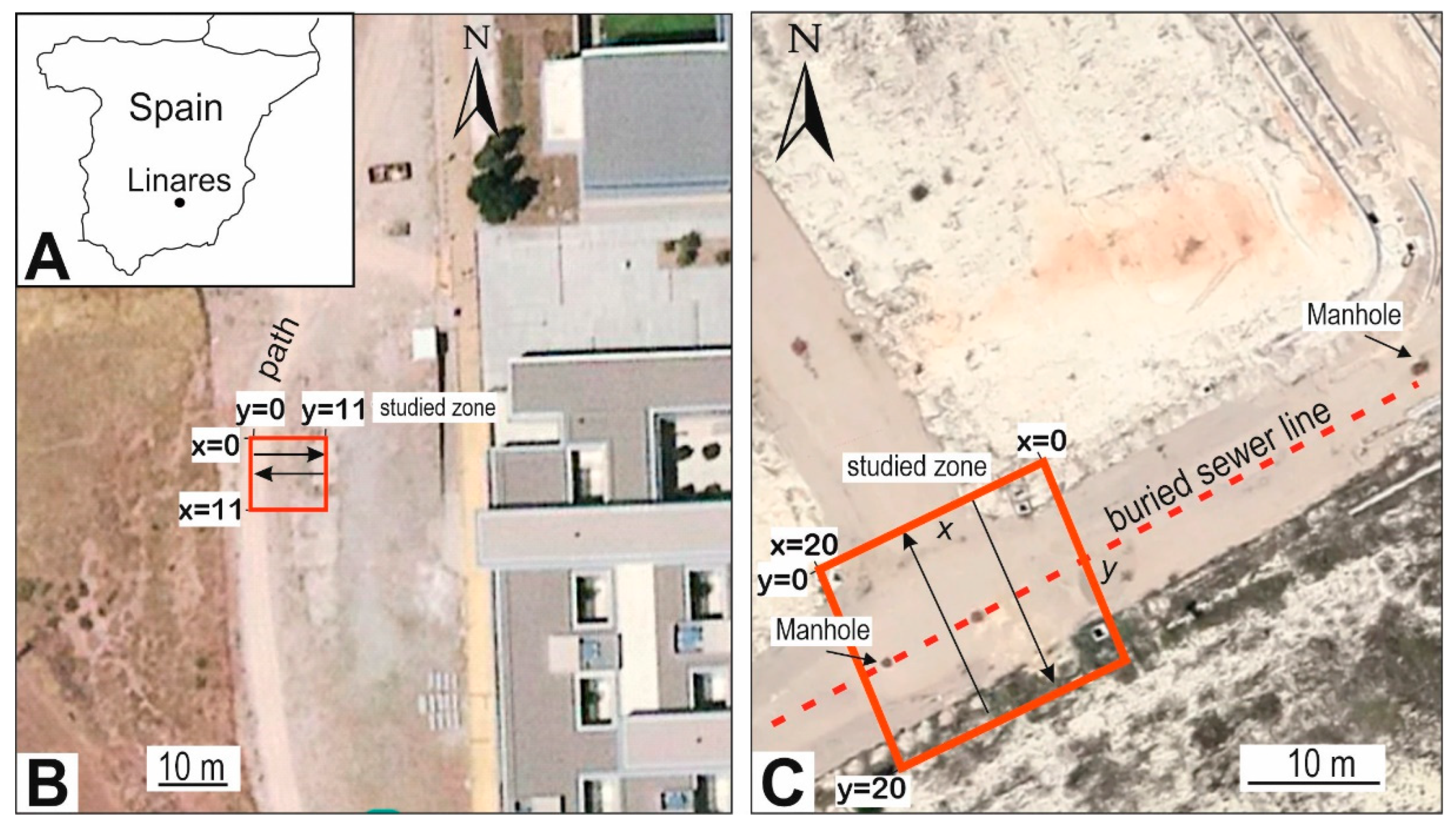
1.2. Study Areas
2. Materials and Methods
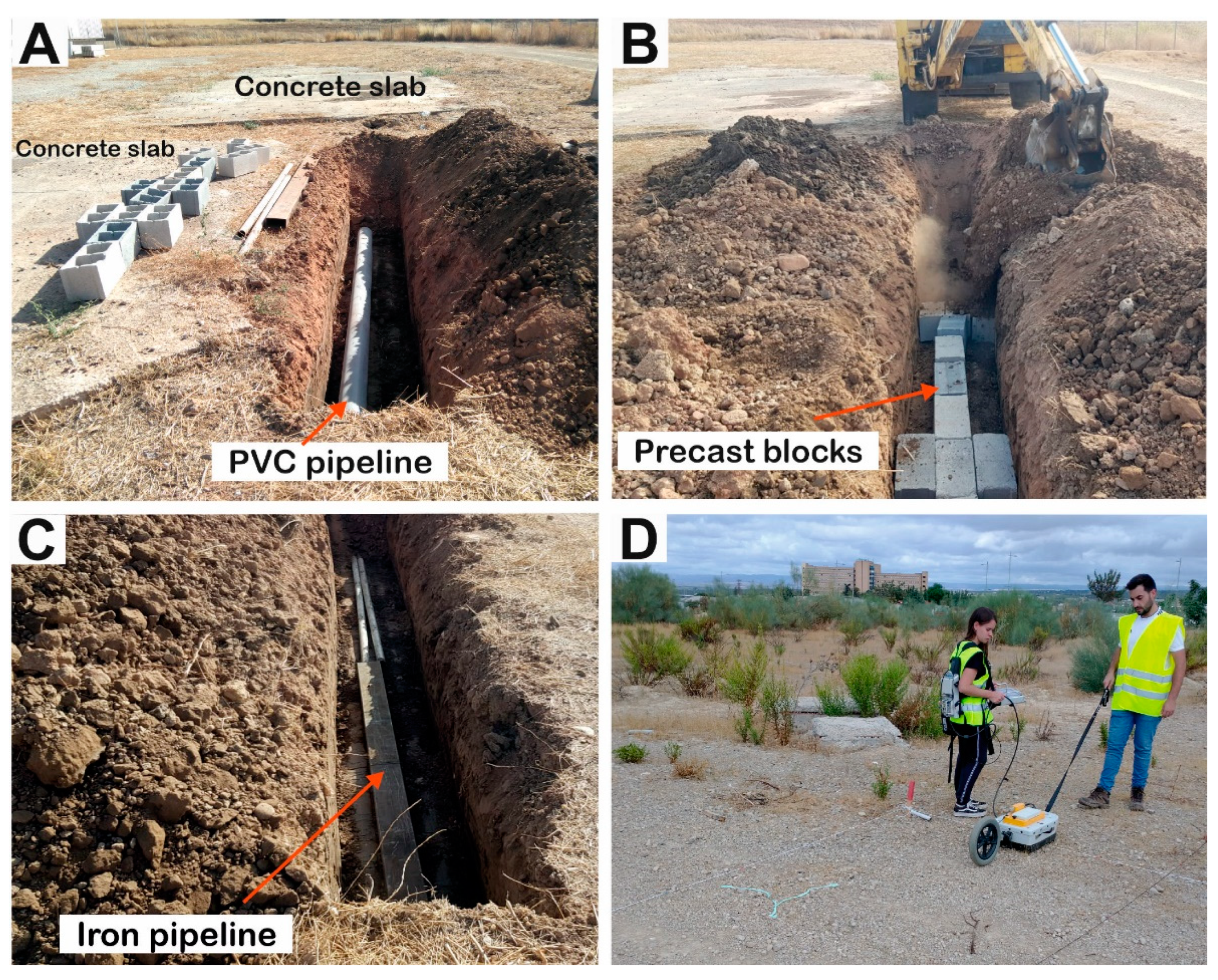
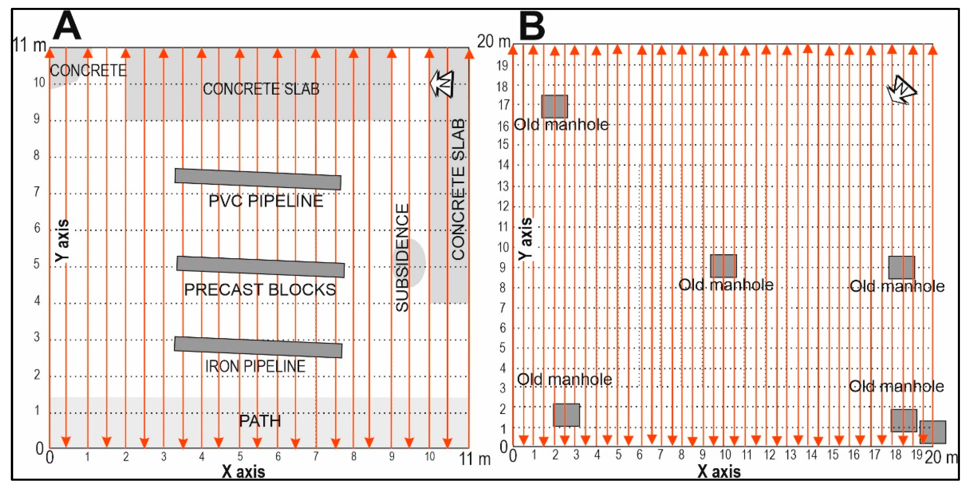
2.1. Experimental Design and Data Acquisition
2.2. Equipment
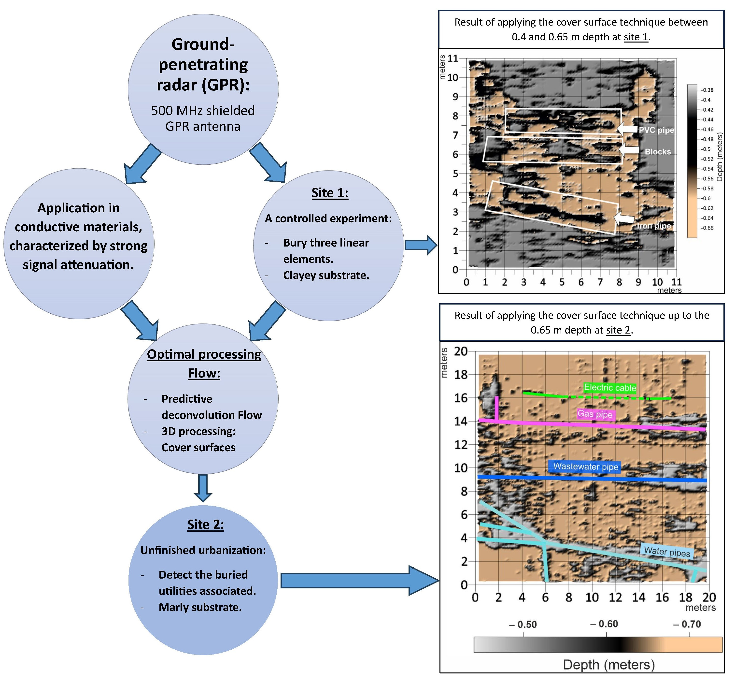
2.3. GPR Data Analysis of Site 1 to Stablish the 2D Processing Flow
2.4. Analysis of Site 1 Using 3D-GPR to Enhance the Coherence Signal
3. Results in Site 2 and Discussion
4. Conclusions
Author Contributions
Funding
Data Availability Statement
Acknowledgments
Conflicts of Interest
References
- Telford, W.M.; Geldart, L.P.; Sheriff, R.E. Applied Geophysics; Cambridge University Press: Cambridge, UK, 1990; 770p. [Google Scholar]
- Annan, A.P. Ground Penetrating Radar: Principles, Procedures & Applications; Sensors & Software Incorporated: Mississauga, QN, Canada, 2003; 278p. [Google Scholar]
- Daniels, D.J. Ground penetrating radar. In The Institution of Electrical Engineers, 2 ed.; Engineers: London, UK, 2004; 726p, Available online: http://refhub.elsevier.com/S0963-8695(17)30017-8/sbref8 (accessed on 15 January 2023).
- Gómez-Ortiz, D.; Martín-Crespo, T.; Martín-Velázquez, S.; Martínez-Pagán, P.; Higueras, H.; Manzano, M. Application of ground penetrating radar (GPR) to delineate clay layers in wetlands. A case study in the Soto Grande and Soto Chico watercourses, Doñana (SW Spain). J. Appl. Geophys. 2010, 72, 107–113. [Google Scholar] [CrossRef]
- Reynolds, J.M. An Introduction to Applied and Environmental Geophysics; John Wiley and Sons Ltd.: Chichester, UK, 2011; 796p. [Google Scholar]
- Neal, A. Ground-penetrating radar and its use in sedimentology: Principles, problems and progress. Earth-Sci. Rev. 2004, 66, 261–330. [Google Scholar] [CrossRef]
- Jol, H.M. Ground Penetrating Radar Theory and Applications; Elsevier Science: Amsterdam, The Netherlands, 2009; 544p. [Google Scholar]
- Pueyo-Anchuela, O.; Pocoví, A.; Casas-Sainz, A.M. Characterization of karst hazards from the perspective of the doline triangle using GPR—Examples from Central Ebro Basin (Spain). Eng. Geol. 2009, 108, 225–236. [Google Scholar] [CrossRef]
- Grangeia, C.; Ávila, P.; Matias, M.; Ferreira da Silva, E. Mine tailings integrated investigations: The case of Rio tailings (Panasqueira Mine, Central Portugal). Eng. Geol. 2011, 123, 359–372. [Google Scholar] [CrossRef]
- Martínez-Moreno, F.J.; Galindo-Zaldívar, J.; Pedrera, A.; Teixido, T.; Ruano, P.; Peña, J.A.; González-Castillo, L.; Ruiz-Constán, A.; López-Chicano, M.; Martín-Rosales, W. Integrated geophysical methods for studying the karst system of Gruta de las Maravillas (Aracena, Southwest Spain). J. Appl. Geophys. 2014, 107, 149–162. [Google Scholar] [CrossRef]
- Cortada, U.; Martínez, J.; Rey, J.; Hidalgo, M.C.; Sandoval, S. Assessment of tailings pond seals using geophysical and hydrochemical techniques. Eng. Geol. 2017, 223, 59–70. [Google Scholar] [CrossRef]
- Galdón, J.M.; Rey, J.; Martínez, J.; Hidalgo, M.C. Application of geophysical prospecting techniques to evaluate geological-mining heritage: The Sinapismo mine (La Carolina, Southern Spain). Eng. Geol. 2017, 218, 152–161. [Google Scholar] [CrossRef]
- Duarte, J.; Cunha, M.; Carvalho, J. Modeling and Comparison of Data Obtained by GPR, for Geological/Structural Analysis of a Carbonated Ornamental Rock Quarry—Blocometry Validation—Case Study in Valinho De Fátima, Portugal. In IOP Conference Series: Earth and Environmental Science, Proceedings of the 6th World Multidisciplinary Earth Sciences Symposium, Prague, Czech Republic, 7–11 September 2020; IOP Publishing: Philadelphia, PA, USA, 2020; p. 609. [Google Scholar] [CrossRef]
- Rey, J.; Mendoza, M.; Martínez, J.; Hidalgo, M.C.; Florez Rodríguez, C. Combining geophysical methods (DC, IP, TDEM and GPR) to characterize mining waste in the Linares-La Carolina district (southern Spain). J. Environ. Manag. 2022, 322, 104921. [Google Scholar] [CrossRef]
- Oliveira, R.J.; Caldeira, B.; Teixidó, T.; Borges, J.F.; Carneiro, A. Increasing the Lateral Resolution of 3D-GPR Datasets through 2D-FFT Interpolation with Application to a Case Study of the Roman Villa of Horta da Torre (Fronteira, Portugal). Remote Sens. 2022, 14, 4069. [Google Scholar] [CrossRef]
- Benedetto, A.; Pajewski, L. Civil Engineering Applications of Ground Penetrating Radar; Springer Transactions in Civil and Environmental Engineering; Springer International: New York, NY, USA, 2015. [Google Scholar]
- Prego, F.J.; Solla, M.; Puente, I.; Arias, P. Efficient GPR data acquisition to detect underground pipes. NDTE Int. 2017, 91, 22–31. [Google Scholar] [CrossRef]
- Wai-Lok Lai, W.; Dérobert, X.; Annan, P.A. Review of Ground Penetrating Radar application in civil engineering: A 30-year journey from Locating and Testing to Imaging and Diagnosis. NDTE Int. 2018, 96, 58–78. [Google Scholar] [CrossRef]
- Pajewski, L.; Fontul, S.; Solla, M. Ground-penetrating radar for the evaluation and monitoring of transport infrastructures. In Innovation in Near-Surface Geophysics. Instrumentation, Application, and Data Processing Methods; Elsevier: Amsterdam, The Netherlands, 2019; pp. 341–398. [Google Scholar]
- Rathod, H.; Debeck, S.; Gupta, R.; Chow, B. Applicability of GPR and a rebar detector to obtain rebar information of existing concrete structures. Case Stud. Constr. Mater. 2019, 11, e00240. [Google Scholar] [CrossRef]
- Solla, M.; Pérez-Gracia, V.; Fontul, S.A. Review of GPR Application on Transport Infrastructures: Troubleshooting and Best Practices. Remote Sens. 2021, 13, 672. [Google Scholar] [CrossRef]
- Neto, P.X.; Medeiros, W.E. A practical approach to correct attenuation effects in GPR data. J. Appl. Geophys. 2006, 59, 140–151. [Google Scholar] [CrossRef]
- Peng, Z.; Jing, G.; Wang, S.; Li, Y.; Guo, Y. Railway ballast layer inspection with different GPR antenas and frequencies. Transp. Geotech. 2022, 36, 100823. [Google Scholar] [CrossRef]
- Liu, Z.; Yeoh, J.K.W.; Gu, X.; Dong, Q.; Chen, Y.; Wu, W.; Wang, L.; Wang, D. Automatic pixel-level detection of vertical cracks in asphalt pavement based on GPR investigation and improved mask R-CNN. Autom. Constr. 2023, 146, 104689. [Google Scholar] [CrossRef]
- Liu, Z.; Gu, X. Performance evaluation of full-scale accelerated pavement using NDT and laboratory tests: A case study in Jiangsu, China. Case Stud. Constr. Mater. 2023, 18, e02083. [Google Scholar] [CrossRef]
- Liu, Z.; Gu, X.; Yang, H.; Wang, L.; Chen, Y.; Wang, D. Novel YOLOv3 model with structure and hyperparameter optimization for detection of pavement concealed cracks in GPR images. IEEE Trans. Intell. Transp. Syst. 2022, 23, 22258–22268. [Google Scholar] [CrossRef]
- Liu, Z.; Gu, X.; Chen, J.; Wang, D.; Chen, Y.; Wang, L. Automatic recognition of pavement cracks from combined GPR B-scan and C-scan images using multiscale feature fusion deep neural networks. Autom. Constr. 2023, 146, 104698. [Google Scholar] [CrossRef]
- Hou, F.; Rui, X.; Fan, X.; Zhang, H. Review of GPR Activities in Civil Infrastructures: Data Analysis and Applications. Remote Sens. 2023, 14, 5972. [Google Scholar] [CrossRef]
- Borgioli, G.; Capineri, L.; Falorni, P.; Matucci, S.; Windsor, C.G. The Detection of Buried Pipes from Time-of-Flight Radar Data. IEEE Trans. Geosci. Remote Sens. 2008, 46, 2254–2266. [Google Scholar] [CrossRef]
- Rashed, M.A.; Al-Garni, M.A. On the application of GPR for locating underground utilities in urban areas. Arab. J. Geosci. 2012, 6, 3505–3511. [Google Scholar] [CrossRef]
- De Coster, A.; Pérez Medina, J.L.; Nottebaere, M.; Alkhalifeh, K.; Neyt, X.; Vanderdonckt, J.; Lambot, S. Towards an improvement of GPR-based detection of pipes and leaks in water distribution networks. J. Appl. Geophys. 2019, 162, 138–151. [Google Scholar] [CrossRef]
- Takahashi, K.; Preetz, H.; Igel, J. Soil properties and performance of landmine detection by metal detector and ground-penetrating radar—Soil characterisation and its verification by a field test. J. Appl. Geophys. 2011, 73, 368–377. [Google Scholar] [CrossRef]
- Cassidy, N.J. Electrical and Magnetic Properties of Rocks, Soils and Fluids. In Ground Penetrating Radar: Theory and Applications; Elsevier: Amsterdam, The Netherlands, 2009; pp. 41–72. [Google Scholar]
- Annan, A.P. Transmission dispersion and GPR. J. Environ. Eng. Geophys. 1996, 1, 125–136. [Google Scholar] [CrossRef]
- Annan, A.P. Ground-penetrating radar. In Near-Surface Geophysics; Society of Exploration Geophysicists: Tulsa, OK, USA, 2005; pp. 357–438. [Google Scholar]
- Ward, S.H.; Hohmann, G.W. Electromagnetic theory for geophysical applications. In Electromagnetic Methods in Applied Geophysics, Vol. 1, Theory; Nabighian, M.N., Ed.; Society of Exploration Geophysicists: Tulsa, OK, USA, 1998; pp. 131–312. [Google Scholar]
- Grimm, R.E.; Heggy, E.; Clifford, S.M.; Dinwiddlie, C.; McGinnis, R.; Farrell, D. Absorption and scattering in ground-penetrating radar: Analysis of the Bishop tuff. J. Geophys. Res. 2006, 11, E06S02. [Google Scholar] [CrossRef] [Green Version]
- Sandmeier, K.J. Program for the Processing of Seismic, Acoustic or Electromagnetic Reflection, Refraction and Transmission Data; REFLEXW Version 7.0; Software Manual; Sandmeier Geophysical Researcher: Karlsruhre, Germany, 2012; Available online: https://www.sandmeier-geo.de/reflexw.html (accessed on 15 January 2023).
- Peña, J.A.; Teixidó, T. Cover Surfaces as a New Technique for 3D GPR Image Enhancement. Archaeological Applications. 2013. Available online: http://hdl.handle.net/10481/22949 (accessed on 25 January 2023).
- Federal Communications Commission (FCC). Title 47—Telecommunication: Volume 1, Part 15, Section 15.509. 2021. Available online: https://www.ecfr.gov/current/title-47/chapter-I/subchapter-A/part-15/subpart-F/section-15.509 (accessed on 15 July 2023).
- Federal Communications Commission (FCC). Title 47—Telecommunication: Volume 1, Part 15, Section 15.209. 2021. Available online: https://www.ecfr.gov/current/title-47/chapter-I/subchapter-A/part-15/subpart-C/section-15.209 (accessed on 15 July 2023).
- American National Standards Institute (ANSI). American National Standard for Methods of Measurement of Radio-Noise Emissions from Low-Voltage Electrical and Electronic Equipment in the Range of 9 kHz to 40 GHz. In ANSI C63.4-2014 (Revision of ANSI C63.4-2009). 2014, pp. 1–170. Available online: https://ieeexplore.ieee.org/document/6840852 (accessed on 25 January 2023).
- Aerotech Telub: EMC test, 500MHz Shielded antenna. Ref: E014-TR020223. Mala Geoscience AB. 2002. Available online: https://fcc.report/FCC-ID/QLA500MHZ/290495.pdf (accessed on 15 July 2023).
- Pereira, M.; Rial, F.I.; Lorenzo, H.; Arias, P.; Novo, A. Analysis of Characteristics of Ground Penetrating Radar Antennas. In Natural Resources & Environmental Engineering, EUET Forestal; University of Vigo: Vigo, Spain, 2006. [Google Scholar]
- Jordan, E.C.; Balmain, K.G. Electromagnetic Waves and Radiating Systems; Prentice-Hall International, INC: Englewood Cliffs, NJ, USA, 1968; 753 p. [Google Scholar]
- Balanis, C.A. Antenna Theory: Analysis and Design; John Wiley & Sons: Hoboken, NJ, USA, 2016. [Google Scholar]
- Cheng, D.K. Field and Wave Electromagnetics; Pearson Education India: Noida, India, 1989. [Google Scholar]
- Conyers, L.B.; Goodman, D. Ground-Penetrating Radar: An Introduction for Archaeologists; AltaMira Press: Lanham, MD, USA, 1997. [Google Scholar]
- Fisher, A.J.; Lowe, D.J. (Eds.) Ground Penetrating Radar in Sediments; Geological Society of London: London, UK, 2004. [Google Scholar]
- Matsuoka, T.; Takeda, H. Ground Penetrating Radar (GPR) Surveys for Railway Ballast Evaluation. J. Appl. Geophys. 2012, 78, 48–56. [Google Scholar]
- Sato, M.; Tsuchiya, N.; Yonezawa, C.; Sato, S. Attenuation Characteristics of GPR Signals in Pavement and Subsurface Structure. J. Appl. Geophys. 2004, 55, 117–130. [Google Scholar]


| Main GPR Acquisition Parameters | ||
|---|---|---|
| Parameters | Site 1 | Site 2 |
| Profile spacing | 0.5 m | 0.5 m |
| Number of profiles | 23 | 41 |
| Trace spacing | 0.01 m | 0.01 m |
| Time window | 30 ns | 40 ns |
| Samples trace | 248 | 312 |
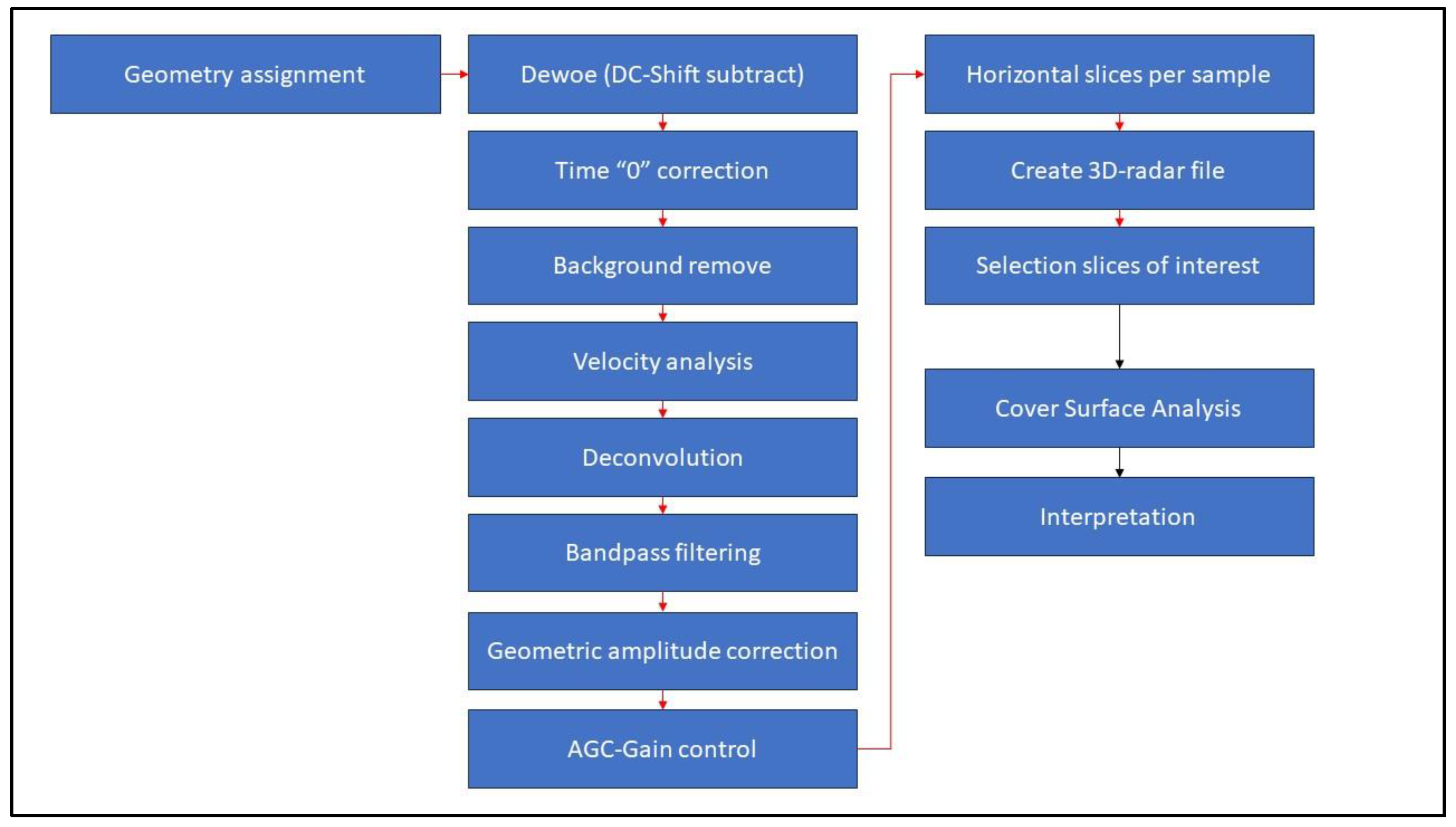
| Steps | Description |
|---|---|
| Subtract DC shift | To eliminate the residual voltage |
| Static correction | To adjust the delay time at time = 0 ns |
| Remove the background noise | To eliminate the multiples proceed by coupled wave (air-surface) |
| Spiking predictive deconvolution | To eliminate additional multiples caused by other superficial structures and increase the high-frequency content; Operator length of 21 ns, predication lag of 7 ns, pre-whitening 10% |
| Bandpass filter | 50 MHz–550 MHz to eliminate the high and low noise frequencies |
| Geometric amplitude correction | To restitute the amplitude content for wave front propagation |
| Gain control (GC) | To increase the amplitude between 10–30 ns where the buried structures are placed; a gain function was created by modifying the AGC |
Disclaimer/Publisher’s Note: The statements, opinions and data contained in all publications are solely those of the individual author(s) and contributor(s) and not of MDPI and/or the editor(s). MDPI and/or the editor(s) disclaim responsibility for any injury to people or property resulting from any ideas, methods, instructions or products referred to in the content. |
© 2023 by the authors. Licensee MDPI, Basel, Switzerland. This article is an open access article distributed under the terms and conditions of the Creative Commons Attribution (CC BY) license (https://creativecommons.org/licenses/by/4.0/).
Share and Cite
Mendoza, R.; Araque-Perez, C.; Marinho, B.; Rey, J.; Hidalgo, M.C. Processing GPR Surveys in Civil Engineering to Locate Buried Structures in Highly Conductive Subsoils. Remote Sens. 2023, 15, 4019. https://doi.org/10.3390/rs15164019
Mendoza R, Araque-Perez C, Marinho B, Rey J, Hidalgo MC. Processing GPR Surveys in Civil Engineering to Locate Buried Structures in Highly Conductive Subsoils. Remote Sensing. 2023; 15(16):4019. https://doi.org/10.3390/rs15164019
Chicago/Turabian StyleMendoza, Rosendo, Carlos Araque-Perez, Bruna Marinho, Javier Rey, and Mari Carmen Hidalgo. 2023. "Processing GPR Surveys in Civil Engineering to Locate Buried Structures in Highly Conductive Subsoils" Remote Sensing 15, no. 16: 4019. https://doi.org/10.3390/rs15164019